Three-dimensional shape reconstruction from images blurred by motion

Wei-Hung Su; Chao-Kuei Lee

doi:10.1117/1.3180865

1 July 2009 Three-dimensional shape reconstruction from images blurred by motion

Wei-Hung Su, Chao-Kuei Lee

Author Affiliations +

Optical Engineering, Vol. 48, Issue 7, 073604 (July 2009). https://doi.org/10.1117/1.3180865

Abstract

Most 3-D shape measurements for a dynamic object always require that the obtained images not be blurred by motion. We show that it is not necessary to avoid the blurred image when projected fringe profilometry is employed. For objects that move within one period of the projected fringes, 3-D surfaces can be retrieved directly from the blurred fringes. Consequently, the presented method intensively reduces the cost of the detection system.

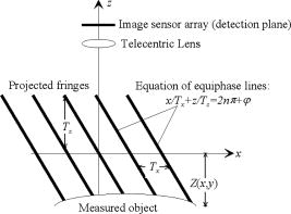
1. Introduction

Three-dimensional shape sensing plays an important role in machine vision, reversed engineering, automatic manufacturing, and other industrial applications. The use of a full-field technique, such as stereovision,^{1, 2} fringe projection,^{3, 4} and structured light illumination,^{5, 6} has been recognized as a promising method for the measurement of a surface profile.

One of the major studies for 3-D sensing is the measurement of dynamic objects. For objects with fast-moving speeds, 3-D shape measurements always require that the observed images not be blurred by motion. High-speed cameras or stroboscopic illuminations are commonly used to obtain unblurred images. Unfortunately, when the speed of the objects still exceeds the temporal resolution of the sensor, the image is blurred. Of course, an ultra-short laser pulse can still be used to freeze the motion on the image. However, the illumination intensity might not be sufficient to perform large-scale measurements, and the cost of such light sources is generally high.

In this paper, we show that the projected fringe profilometry⁴ does not need to avoid the blurred images. As a typical setup, we use a fringe pattern to illuminate the dynamic object and utilize a CCD camera to record the fringe distribution. Fringes on the obtained image are deformed by the topography of the object and also blurred by motion. Theoretical analysis shows that objects moving within one period of the projected fringe can be directly described by the projected fringe profilometry. Thus, the cost of the detection system is effectively reduced.

2. Theoretical Analysis

Figure 1 shows the system configuration. The $x - z$ plane is located in the figure plane, and the $y$ axis is normal to the figure plane. A fringe pattern is projected onto the inspected surface. Intensity of the fringes when propagating in space is represented as

Eq. 1

I_{f} (x, z) = a + b \cos (\frac{2 π x}{T_{x}} + \frac{2 π z}{T_{z}}),

where

a

is the background or dc intensity level,

b

is the fringe contrast, and

T_{x}

and

T_{z}

are periods of the fringes in

x

and

z

axis, respectively. The depth value

Z (x, y)

on a surface point is measured relative to the

x - y

plane indicated in the figure. Thus, the reflected intensity

I_{r}

on the surface is expressed as

Eq. 2

I_{r} (x, y) = a R (x, y) + b R (x, y) \cos [\frac{2 π x}{T_{x}} + \frac{2 π Z (x, y)}{T_{z}}],

where

R (x, y)

is the reflectivity of the measured object.

Fig. 1

Schematic setup of projected fringe profilometry.

The projected fringes on the surface are observed by the image sensor array. The detection plane coordinate system $(r, c)$ is defined in the CCD detection plane with $r$ and $c$ axes parallel to the row and the column directions of the sensor array, respectively. The gray level on the recorded image corresponding to $I_{r} (x, y)$ is described as

Eq. 3

I (r, c) = A_{1} (r, c) + B_{1} (r, c) \cos φ_{Z} (r, c),

where

A_{1} (r, c)

is the background or dc gray level,

B_{1} (r, c)

is the modulation amplitude, and

φ_{Z} (r, c)

is the measured absolute phase. For a telecentric system, the mapping transformation between the image plane and

x - y

plane is

Eq. 4

{\begin{matrix} r = M x \\ c = M y \end{matrix},

where

M

is the magnitude of the telecentric lens. A phase value sampled at an object point is assumed equal to that sampled at its image point. This assumption applies when the point spread function of the system is symmetric (coma-free). Thus, Eq. 3 can then be rewritten as

Eq. 5

I (M x, M y) = A_{1} (r, c) + B_{1} (r, c) \cos φ_{Z} (r, c) = K a R (x, y) + K b R (x, y) \cos [\frac{2 π x}{T_{x}} + \frac{2 π Z (x, y)}{T_{z}}],

where the constant

K

identifies the linear relationship between the reflected light intensity

I_{r}

and the image gray level

I

.

$φ_{Z} (r, c)$ can be extracted with the phase-shifting technique or Fourier transform method. Since both phase evaluation techniques involve the arctangent operation, the extracted phases have discontinuities with $2 π$ phase jumps. Unwrapping is inevitable to recover the absolute phases.⁷ Once the unwrapped phase $φ_{Z} (r, c)$ is obtained, depth on the surface point can be directly found from Eq. 5, as given by

Eq. 6

Z (x, y) = \frac{T_{z}}{2 π} φ_{Z} (c, r) - \frac{T_{z}}{T_{x}} x .

Now, consider this inspected object moving with speed $(υ_{x}, υ_{y}, υ_{z})$ in the world coordinates. Its depth profile is a function of time and is given by

Eq. 7

Z (x, y, t) = Z_{o} (x, y) + \nabla Z_{o} (x, y) \cdot (\hat{x} υ_{x} + \hat{y} υ_{y}) t + υ_{z} t = Z_{o} (x, y) + [υ_{x} \frac{\partial Z_{o} (x, y)}{\partial x} + υ_{y} \frac{\partial Z_{o} (x, y)}{\partial y} + υ_{z}] t,

where

Z_{o} (x, y)

is the object depth function at

t = 0

.

\hat{x}

and

\hat{y}

are unit vectors. ∇ is a 2-D gradient operator, which is denoted as

\nabla = \hat{x} (\partial ∕ \partial x) + \hat{y} (\partial ∕ \partial y)

.

The image sensor array obtains a blurred image within the exposure time $Δ t$ . The gray level of the blurred image with reference to Eq. 5 can be expressed as

Eq. 8

I_{blurred} (M x, M y) = A (r, c) + B (r, c) \cos φ_{blurred} (r, c) = \int_{t = 0}^{t = Δ t} {K a R (x - υ_{x} t, y - υ_{y} t) + K b R (x - υ_{x} t, y - υ_{y} t) \cos [\frac{2 π x}{T_{x}} + \frac{2 π}{T_{z}} Z (x, y, t)]} d t,

where

φ_{blurred} (r, c)

is the measured phase from the blurred fringes,

A (r, c)

is the measured background or dc gray level, and

B (r, c)

is the modulation amplitude.

For objects in which $R (x, y)$ varies slowly with $x$ and $y$ , Eq. 8 can be represented as

Eq. 9

I_{blurred} (M x, M y) = K \int_{t = 0}^{t = Δ t} {a R (x, y) + b R (x, y) \cos [\frac{2 π x}{T_{x}} + \frac{2 π}{T_{z}} Z (x, y, t)]} d t .

Substituting Eq. 7 into Eq. 9, the intensity of the blurred image is then simplified as

Eq. 10

I_{blurred} (M x, M y) = K a R (x, y) Δ t + K b R (x, y) Δ t \cdot sinc (\frac{α Δ t}{T_{z}}) \cos {\frac{2 π x}{T_{x}} + \frac{2 π}{T_{z}} [Z_{o} (x, y) + α Δ t ∕ 2]},

where

α = υ_{x} [\partial Z_{o} (x, y) ∕ \partial x] + υ_{y} [\partial Z_{o} (x, y) ∕ \partial y] + υ_{z}

, and

sinc (x) = \sin (π x) ∕ (π x)

.

According to Eq. 7, the depth profile at $t = Δ t ∕ 2$ can be expressed as

Eq. 11

Z_{1} (x, y) = Z_{o} (x, y) + α Δ t ∕ 2,

and therefore Eq. 10 is represented as

Eq. 12

I_{blurred} (M x, M y) = K a R (x, y) Δ t + K b R (x, y) Δ t \cdot sinc (\frac{α Δ t}{T_{z}}) \cos [\frac{2 π x}{T_{x}} + \frac{2 π}{T_{z}} Z_{1} (x, y)] .

Comparing Eq. 8 with Eq. 12, it is found that

Z_{1} (x, y)

can be fully identified from the blurred fringes, as given by

Eq. 13

Z_{1} (x, y) = \frac{T_{z}}{2 π} φ_{blurred} (x, y) - \frac{T_{z}}{T_{x}} x .

Thus, the 3-D shape of the dynamic object at

t = Δ t ∕ 2

can be directly retrieved from the blurred fringe. If the exposure time

Δ t

is close to zero, Eq. 13 becomes close to Eq. 5, and the fringes are not blurred.

3. Experiments

A ball with moving speed $υ_{x} = 0.62 mm ∕ s$ , $υ_{y} = 0.62 mm ∕ s$ , and $υ_{z} = 0.13 mm ∕ s$ was chosen as the dynamic sample. Its diameter was approximately $40 mm$ . A sinusoidal fringe pattern was illuminated by a halogen lamp and then projected onto this dynamic sample. A CCD camera with $1024 \times 1024 pixels$ at $12 - bit$ pixel resolution was used to record the fringe distribution. Fringes were blurred by linear motion. Figure 2 shows the fringe distribution, in which the exposure time was $4.0 s$ .

Fig. 2

(a) Fringes on the inspected object observed by a CCD camera when the object was shifting along a specific direction. (b) Phase distribution on the dynamic object. A gray-level bar is used to address the phase values.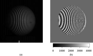

Phase-extraction was performed with the Fourier transform method.³ Figure 2 shows the computed phase $φ_{blurred}$ , which was within the interval between $- π$ and $π$ . Unwrapping was a necessary procedure to eliminate the discontinuities. In our experiment, we use Goldstein’s algorithm⁷ to restore the absolute phases. With Eq. 13, depth profile $Z_{1} (x, y)$ was determined. Figure 3 shows the retrieved profile. Its 1-D profile is shown in Fig. 3.

Fig. 3

(a) Retrieved profile $Z_{1} (x, y)$ for the inspected object. A gray-level bar is used to address the depth values. (b) One-dimensional surface plot of (a).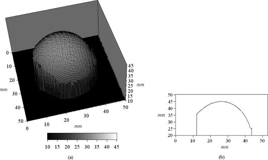

A comparison when the sample was static was performed as well. Appearance of the projected fringes on the static sample is shown as Fig. 4. Equation 6 was employed to retrieve the 3-D shape. Figures 4 and 4 show the retrieved 3-D shape and its 1-D profile, respectively. Systematic accuracy for a static object was approximately $150 μ m$ . The errors were mainly from the spatially sampling density of the CCD camera and phase-extraction. The sampling resolution was approximately $100 μ m$ , which was determined by the field of view and the pixel numbers of the CCD camera.

Fig. 4

(a) Appearance of the fringe distribution when the object was static. (b) Retrieved profile for the inspected object. (c) One-dimensional surface plot of (b).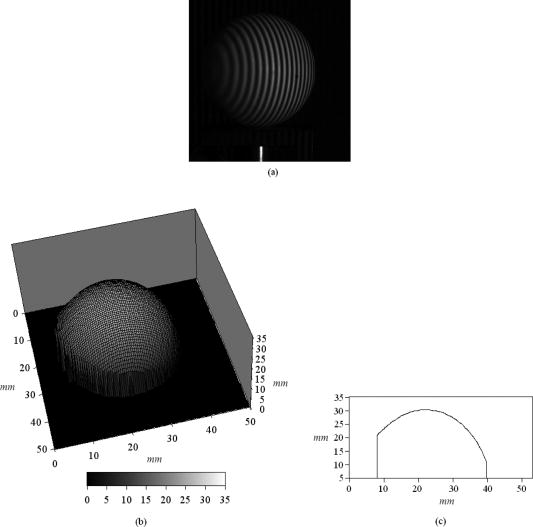

The difference between one two profiles (the dynamic case and the static case) is depicted in Fig. 5, in which the shifting displacement has been compensated. It was found that accuracy at the center area of the sample could be achieved with the same order of the static case, implying that our theoretical analysis was correct. However, enormous errors occurred at the edge of the dynamic object.

Fig. 5

Difference between the profiles in Figs. 3 and 4. Shifting displacement between the two profiles has been compensated.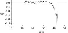

There were two sources causing such errors. They were (1) variation of effective exposure time at the boundary area, and (2) ambiguity of phase-extraction for surfaces with large depth variation. The exposure time for image pixels that inspected the boundary area was unfortunately not a constant. It was highly dependent on the moving direction and the shape of the boundary. For example, a surface point on the boundary is observed by the image sensor array. Since this object is dynamic, the observed point is moving from point $A$ to point $B$ on the detection plane during the exposure time $Δ t$ . As shown in Fig. 6, for a sensor pixel $C$ that is located within the interval between $A$ and $B$ , its effective exposure time is $Δ t \cdot \bar{C B} ∕ \bar{A B}$ . The effective exposure time on the boundary area was therefore not $Δ t$ . Equation 9 was not applicable for the boundary area. The example shown in Fig. 6 also indicates that the effective exposure time was corresponding to the shape of the boundary on the detection plane. Effective exposure time for pixel $D$ in Fig. 6 is different from that for pixel $E$ in Fig. 6.

Fig. 6

Examples of the observed boundary on the detection plane: (a) the circular boundary, and (b) the rectangular boundary.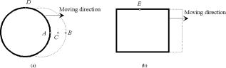

Errors from ambiguity of phase-extraction occur when the shifting amount of the projected fringes is larger than their periods. A displacement of the dynamic object directly causes the projected fringes to shift from one surface point to another. If the shifting amount is equal to the fringe period, the fringe contrast becomes zero. This phenomenon can be mathematically described when the sinc function in Eq. 10 is equal to zero, or say, $α \cdot Δ t$ is equal to $T_{z}$ . In such a situation, phase cannot be identified on that area. Moreover, aliasing occur when the shifting amount is larger than the fringe period, i.e., $α \cdot Δ t > T_{z}$ . This directly causes a $2 π$ phase offset when performing the phase unwrapping. Equation 10 for the aliasing area should be modified as

Eq. 14

I_{blurred} (M x, M y) = K a R (x, y) Δ t + K b R (x, y) Δ t \cdot sinc (\frac{α Δ t}{T_{z}}) \cos {\frac{2 π x}{T_{x}} + \frac{2 π}{T_{z}} [Z_{o} (x, y) + α Δ t ∕ 2] \pm 2 π},

and Eq. 13 is replaced as

Eq. 15

Z_{1} (x, y) = \frac{T_{z}}{2 π} [φ_{blurred} (x, y) \pm 2 π] - \frac{T_{z}}{T_{x}} x .

Since aliasing occurs with

[υ_{x} \frac{\partial Z_{o} (x, y)}{\partial x} + υ_{y} \frac{\partial Z_{o} (x, y)}{\partial y} + υ_{z}] Δ t > T_{z},

distribution of the aliasing area is varied with the moving direction, speed of motion, slope of the profile, and exposure time. We performed several measurements by changing parameters such as the moving direction, the moving speed, and the exposure time. An example is illustrated in Fig. 7. Figures 7 and 7 are appearances of the inspected sample moving along the

x

and

y

axis, respectively. The moving speed was

2.0 mm ∕ s

, and the exposure time of the CCD camera was

2.6 s

. The phase extracted by the Fourier transform method is depicted as Fig. 8. Aliasing areas are enclosed with dotted lines. Ideally, the

2 π

phase offset on the aliasing area could be compensated by adding or reducing a

2 π

phase value. Unfortunately, the signal-to-noise ratio (SNR) was too low around the zero fringe-contrast area, and therefore phase information was lost. This directly made performing the phase extraction uncertain when using the Fourier transform method. The phase distribution became continuous on the boundary between the aliasing area and the unaliasing area. If the phase on the aliasing area was compensated by adding or reducing a

2 π

phase value, discontinuity with a

2 π

phase jump appeared on the zero fringe-contrast area. Thus, it is impractical to robotically recover phases on the aliasing area by simply adding or reducing a

2 π

phase value.

Fig. 7

Appearance of the fringe distribution when the object was shifting along (a) the $x$ axis and (b) the $y$ axi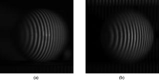s.

Fig. 8

Phase map computed by the Fourier transform method for the object shifting along (a) the $x$ axis and (b) the $y$ axis. Aliasing areas are enclosed with dotted lines.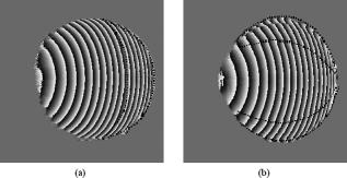

Figure 9 shows the recorded blurred image when the sample was moving along the $z$ axis. The moving speed of the sample was $3.4 mm ∕ s$ , and the exposure time was $1.0 s$ . The retrieved phase is shown in Fig. 9. Since $υ_{x}$ and $υ_{y}$ were zero, the value $α$ was only a function of $υ_{z} Δ t$ . Fringe contrast over the whole image was therefore varied only with $υ_{z} Δ t$ , not with $x$ or $y$ . Phase extraction did not encounter any ambiguity. Sources of errors corresponding to various moving directions are reported in Table 1.

Fig. 9

(a) Appearance of the fringe distribution when the object was shifting along the $z$ axis. (b) Phase distribution on the dynamic object.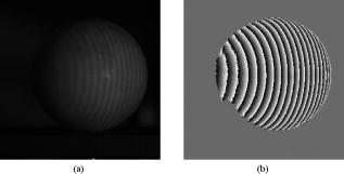

Table 1

Sources of errors caused by the moving direction.


Movingvector	$\hat{x} υ_{x}$	$\hat{y} υ_{y}$	$\hat{z} υ_{z}$	$\hat{x} υ_{x} + \hat{y} υ_{y} + \hat{z} υ_{z}$
Distributionof the zerofringecontrast	$υ_{x} \frac{\partial Z_{0} (x, y)}{\partial x} \cdot Δ t$ $= T_{z}$	$υ_{y} \frac{\partial Z_{0} (x, y)}{\partial y} \cdot Δ t$ $= T_{g}$	$υ_{z} \cdot Δ t = T_{z}$	$[υ_{x} \frac{\partial Z_{0} (x, y)}{\partial x} + υ_{y} \frac{\partial Z_{0} (x, y)}{\partial y} + υ_{z}] Δ t$ $= T_{z}$
Area withphaseuncertainty	Aliasing area andarea with zerofringe contrast	Aliasing area andarea with zerofringe contrast	Area withzero fringecontrast	Aliasing area and area with zero fringecontrast
Area withenormousmeasurementerrors	Edge area, aliasingarea, and area withzero fringe contrast	Edge area, aliasingarea, and area withzero fringe contrast	Edge areaand areawith zerofringecontrast	Edge area, aliasing area, and area withzero fringe contrast

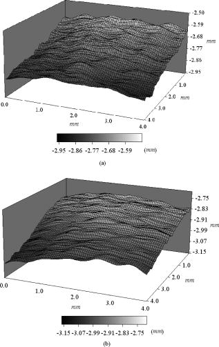
Systematic accuracy for a dynamic object can be illustrated as Fig. 10, in which a plate moving along the $z$ axis was inspected. The roughness of this plate was approximately $10 μ m$ . The moving speed was $2.9 mm ∕ s$ , and the exposure time was $1.0 s$ . A comparison was evaluated when this plate was static, as shown in Fig. 10. The retrieved 3-D shape for the dynamic case and the static case is depicted as Figs. 11 and 11, respectively. Even though the fringe contrast on the dynamic object was relatively low, its profile can be retrieved with accuracy as high as the static one.

Fig. 10

Appearances of the fringe distributions when (a) the plate was shifting along the $z$ axis and (b) the plate was static.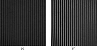

Fig. 11

Retrieved 3-D shapes for (a) the moving plate and (b) the static plate.

Compared with other methods using deblurred algorithms to restore the observed information, the proposed method saves the computation time. For approaches using a high-speed camera or stroboscopic illuminations to freeze the object’s motion, the cost of the proposed system is relatively low. However, limitations are that the inspected object should be a rigid body, and this object should move linearly within one period of the projected fringes. If the displacement of the projected fringes shifts larger than one period of the fringes, aliasing will occur. In addition, errors also occur when the inspected object is rotating. Equation 9 is not applicable when the moving vector is time-dependent.

4. Conclusions

We have presented a discussion on how to retrieve the 3-D shape from an image blurred by motion. With the fringe projection method, objects moving within one period of the projected fringes can be fully described. Thus, it is not necessary to avoid blurred images. Accuracy can be achieved that is as high as with the static image. This makes it desirable to reduce the cost of the detection system. We believe that applications to microelectromechanical systems (MEMS) and biomedical inspections can be realized.

References

1.

N. A. Thacker and J. E. W. Mayhew, “Optimal combination of stereo camera calibration from arbitrary stereo images,” Image Vis. Comput., 9 27 –32 (1990). https://doi.org/10.1016/0262-8856(91)90045-Q 0262-8856 Google Scholar

2.

R. A. Lane, N. A. Thacker, and N. L. Seed, “Stretch-correlation as a real-time alternative to feature-based stereo matching algorithms,” Image Vis. Comput., 12 203 –212 (1994). https://doi.org/10.1016/0262-8856(94)90074-4 0262-8856 Google Scholar

3.

M. Takeda and K. Mutoh, “Fourier transform profilometry for the automatic measurement of 3-D shaped object,” Appl. Opt., 22 3977 –3982 (1983). https://doi.org/10.1364/AO.22.003977 0003-6935 Google Scholar

4.

V. Srinivasan, H. C. Liu, and M. Halioua, “Automated phase-measuring profilometry of 3-D diffuse objects,” Appl. Opt., 23 3105 –3108 (1984). https://doi.org/10.1364/AO.23.003105 0003-6935 Google Scholar

5.

W. H. Su, “Color-encoded fringe projection for 3D shape measurements,” Opt. Express, 15 13167 –13181 (2007). https://doi.org/10.1364/OE.15.013167 1094-4087 Google Scholar

6.

W. H. Su, “Projected fringe profilometry using the area-encoded algorithm for spatially isolated and dynamic objects,” Opt. Express, 16 2590 –2596 (2008). https://doi.org/10.1364/OE.16.002590 1094-4087 Google Scholar

7.

E. Zappa and G. Busca, “Comparison of eight unwrapping algorithms applied to Fourier-transform profilometry,” Opt. Lasers Eng., 46 106 –116 (2008). https://doi.org/10.1016/j.optlaseng.2007.09.002 0143-8166 Google Scholar

Biography

Wei-Hung Su is an assistant professor in the Department of Material Science and Optoelectronic Engineering at the National Sun Yat-Sen University, Taiwan. He earned a PhD degree and an MS degree in electrical engineering from Pennsylvania State University in 2002 and 1999, respectively. His professional interests are optical metrology, digital image processing, and optical information processing.

Chao-Kuei Lee received his PhD in electro-optical engineering from National Chiao Tung University, Taiwan, in 2003. He is currently an assistant professor who directs the Laboratory of Femtosecond and Quantum Modulation with the Institute of Electro-Optical Engineering in National Sun Yat-sen University. His research interests include femotosecond light sources, ultrafat optoelectronics, and coherent quantum control.

Citation Download Citation

Wei-Hung Su and Chao-Kuei Lee "Three-dimensional shape reconstruction from images blurred by motion," Optical Engineering 48(7), 073604 (1 July 2009). https://doi.org/10.1117/1.3180865

Published: 1 July 2009

Access the abstract

JOURNAL ARTICLE
7 PAGES

DOWNLOAD PAPER SAVE TO MY LIBRARY

GET CITATION

CITATIONS

Cited by 5 scholarly publications.

Explore citations on Lens.org

RIGHTS & PERMISSIONS

Get copyright permission Get copyright permission on Copyright Marketplace

KEYWORDS

3D image processing

Inspection

3D image reconstruction

Fringe analysis

CCD cameras

Optical engineering

Fourier transforms

1.

Introduction

2.

Theoretical Analysis

Eq. 1

Eq. 2

Fig. 1

Eq. 3

Eq. 4

Eq. 5

Eq. 6

Eq. 7

Eq. 8

Eq. 9

Eq. 10

Eq. 11

Eq. 12

Eq. 13

3.

Experiments

Fig. 2

Fig. 3

Fig. 4

Fig. 5

Fig. 6

Eq. 14

Eq. 15

Fig. 7

Fig. 8

Fig. 9

Table 1

Fig. 10

Fig. 11

4.

Conclusions

References

Biography

Show All Keywords

Keywords/Phrases

Search In:

Publication Years