Object tracking using an adaptive Kalman filter combined with mean shift

Xiaohe Li; Taiyi Zhang; Xiaodong Shen; Jiancheng Sun

doi:10.1117/1.3327281

1 February 2010 Object tracking using an adaptive Kalman filter combined with mean shift

Xiaohe Li, Taiyi Zhang, Xiaodong Shen, Jiancheng Sun

Author Affiliations +

Optical Engineering, Vol. 49, Issue 2, 020503 (February 2010). https://doi.org/10.1117/1.3327281

Abstract

An object tracking algorithm using an adaptive Kalman filter (KF) combined with mean shift (MS) is proposed. First, the system model of KF is constructed, then the center of the object predicted by KF is used as the initial value of the MS algorithm. The searching result of MS is fed back as the measurement of the adaptive KF, and the estimate parameters of KF are adjusted by the Bhattacharyya coefficient adaptively. The proposed method has the robust ability to track a moving object in consecutive frames under certain real-world complex situations, such as a moving object disappearing partially or totally due to occlusion, fast moving objects, and sudden changes in velocity of a moving object. The experimental results demonstrate that the proposed tracking algorithm is robust and practical.

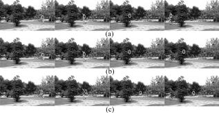
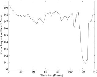
1. Introduction

Object tracking is a common vision task to find and follow moving objects between consecutive frames. It has widespread applications in fields ranging from video coding, visual surveillance, and human computer interaction, to intelligent robotics.

Among numerous object tracking algorithms, mean shift (MS) object tracking has recently received growing interest since it was introduced by Comaniciu, Ramesh, and Meer.¹ This method tracks an object region represented by a spatially weighted intensity histogram. An object function that compares target and candidate kernel densities is formulated using the Bhattacharyya coefficient, and tracking is achieved by optimizing this objective function using the iterative MS algorithm. Though the MS object tracking algorithm performs well on sequences with relatively small object displacement, its performance is not guaranteed when the objects move fast or undergo partial or full occlusion.

To overcome this disadvantage of the MS tracking method, an improved MS object tracking algorithm was proposed in Ref. 2 by initializing MS with the predicted value of a Kalman filter (KF). In Ref. 3, the exact target center is obtained by combining the two estimated target centers obtained by the KF and MS algorithm respectively at each frame. Since the prediction and measurement errors of KF are set as constant, this algorithm is not robust enough. A new object tracking scheme is proposed in Ref. 4 that combines the sum-of-squared-differences object tracking method and MS object tracking method in the KF framework. In this method, to handle partial occlusion, the whole object is represented by a number of elementary MS modules embedded within the object, rather than a single global MS tracker. Therefore, this scheme is time consuming.

In this work, a novel object tracking algorithm based on MS and KF is proposed. First, the system model of KF is constructed, and the center of the object predicted by KF is used as the initial value of the MS algorithm. Then the searching result of MS is fed back as the measurement of KF, and the estimated parameters of KF are adjusted by the Bhattacharyya coefficient adaptively. The proposed algorithm can accurately capture the object’s position when the object undergoes large displacements or occlusion.

The remainder of this work is organized as follows. In Sec. 2, we review MS object tracking briefly. The proposed object tracking algorithm is presented in Sec. 3. Experimental results are given in Sec. 4, followed by conclusions in Sec. 5.

2. Mean Shift Object Tracking

In the MS object tracking method,¹ the target model is defined as its normalized color histogram $q = {q_{u}}_{u = 1, \dots, m}$ , where $m$ is the number of bins. The normalized color distribution of a target candidate $p (y) = {p_{u} (y)}_{u = 1, \dots, m}$ centered at $y$ in the current frame can be calculated as

Eq. 1

p_{u} (y) = C_{h} \sum_{i = 1}^{n_{h}} k ({‖ \frac{y - x_{i}}{h} ‖}^{2}) δ [b (x_{i}) - u],

where

{x_{i}}_{i = 1, \dots, n_{h}}

are the

n_{h}

pixel locations of the target candidate in the target area,

δ

is the Kronecker delta function,

b (x_{i})

associates the pixel

x_{i}

to the histogram bin,

k (x)

is the kernel profile with bandwidth

h

, and

C_{h}

is a normalization constant. The same equations are used to obtain the color distribution of the target model

q

.

The Bhattacharyya coefficient, which evaluates the similarity of the target model and the target candidate model, is defined as

Eq. 2

ρ (y) = ρ [p (y), q] = \sum_{u = 1}^{m} {[p_{u} (y) q_{u}]}^{1 ∕ 2} .

To find the location corresponding to the target in the current frame, the Bhattacharyya coefficient in Eq. 2 should be maximized as a function of $y$ , which can be solved by running the MS iterations. We assume that the search for the new target location in the current frame starts at the location $y_{0}$ . At each step of the iterative process, the estimated target moves from $y_{0}$ to the new location $y_{1}$ , defined as

Eq. 3

y_{1} = \frac{\sum_{i = 1}^{n_{h}} x_{i} w_{i} g ({‖ (y_{0} - x_{i}) ∕ h ‖}^{2})}{\sum_{i = 1}^{n_{h}} w_{i} g ({‖ (y_{0} - x_{i}) ∕ h ‖}^{2})},

where

Eq. 4

w_{i} = \sum_{u = 1}^{m} {[\frac{q_{u}}{p_{u} (y_{0})}]}^{1 ∕ 2} δ [b (x_{i}) - u],

and

g (x) = - k^{'} (x)

. More information on MS object tracking can be found in Ref. 1.

3. Adaptive Kalman Filter for Object Tracking

In this work, the MS object tracking method is integrated into the KF framework, and an adaptive KF algorithm for object tracking is proposed. First, MS initialized by the predicted value of KF is used to search the target position. Then the searching result of MS is fed back as the measurement of KF, and the estimated parameters of KF are adjusted by the Bhattacharyya coefficient adaptively. For faster implementation, two independent trackers of KF were defined for horizontal and vertical movement.

3.1.

Model of the Kalman Filter

We define the variable as the discrete time $t$ , state vector $X (t)$ , measurement vector $Z (t)$ , state transition matrix $A$ , measurement matrix $C$ , state noise $ν (t)$ , and measurement noise $μ (t)$ . The system is expressed as:

Eq. 5

{\begin{cases} X (t) = A X (t - 1) + ν (t - 1) \\ Z (t) = C X (t) + μ (t) \end{cases} .

We assume that $ν (t - 1)$ and $μ (t)$ are Gaussian random variable with zero mean, so their probability density functions are $N [0, Q (t - 1)]$ and $N [0, R (t)]$ , where the covariance matrix $Q (t - 1)$ and $R (t)$ are referred to as the transition noise covariance matrix and measurement noise covariance matrix.

We design a model to track object (the details are as follows). The state vector is $X = {(x, v, a)}^{T}$ , where $x, v$ , and $a$ represent the (horizontal or vertical) center, velocity, and acceleration, respectively. The measurement vector is $Z = x$ . The state transition matrix is

Eq. 6

A = (\begin{matrix} 1 & Δ t & 0.5 Δ t^{2} \\ 0 & 1 & Δ t \\ 0 & 0 & 1 \end{matrix}),

where

Δ t

is the time interval. The measurement matrix is

C = (1, 0, 0)

. The transition noise covariance matrix is

Eq. 7

Q (t - 1) = [\begin{matrix} σ_{1}^{2} (t - 1) & 0 & 0 \\ 0 & 0.5 σ_{1}^{2} (t - 1) & 0 \\ 0 & 0 & 0.2 σ_{1}^{2} (t - 1) \end{matrix}],

and the measurement noise covariance is

R (t) = σ_{2}^{2} (t)

. The estimate of parameters

σ_{1}^{2} (t)

and

σ_{2}^{2} (t)

is described in Sec. 3.2.

3.2.

Adaptive Kalman Filter

In the KF algorithm, the measurement error covariance $R (t)$ and Kalman gain are in inverse ratio. As the covariance matrix $R (t)$ approachs zero, the Kalman gain weights the residual more heavily. In this case, the measurement is trusted more and more, while the predicted result is trusted less and less. On the other hand, as the a-priori estimate error covariance of KF approaches zero, the Kalman gain weights the residual less heavily. The actual measurement is trusted less and less, while the predicted result is trusted more and more.⁵ Therefore, the system will achieve a near optimal result if we can decide which one to trust. In this work, the so-called adaptive KF allows the estimated parameters $R (t)$ and $Q (t - 1)$ of KF to adjust automatically according to the Bhattacharyya coefficient of MS object tracking.

In the MS object tracking method, the Bhattacharyya coefficient evaluates the similarity of the target and candidate models. When the tracked object is occluded by other objects or background, the Bhattacharyya coefficient will descend dramatically. Thus, we define a threshold $T_{h}$ to determine whether the occlusion happens or not.

Assuming the searching result of MS is ${\hat{y}}_{t}$ in the current frame $t$ , the Bhattacharyya coefficient $ρ ({\hat{y}}_{t})$ evaluates the similarity of the target model and the candidate model centered at ${\hat{y}}_{t}$ . Since the search result of MS is used as a measurement of KF, in a correction step the Bhattacharyya coefficient is used to adjust the estimate parameters of adaptive KF. If the Bhattacharyya coefficients $ρ ({\hat{y}}_{t})$ is more than the threshold $T_{h}$ , then the value of $σ_{1}^{2} (t - 1)$ is set as $ρ ({\hat{y}}_{t})$ , and $σ_{2}^{2} (t)$ is $1 - ρ ({\hat{y}}_{t})$ . Otherwise, it is reasonable to let $σ_{1}^{2} (t - 1)$ and $σ_{2}^{2} (t)$ be zero and infinity, respectively, thus the Kalman gain is a zero value. To smooth temporal variations, the parameters associated with the current frame are obtained through temporal filtering,

Eq. 8

{\begin{cases} σ_{1}^{2} (t - 1) = (1 - λ) {\hat{σ}}_{1}^{2} (t - 1) + λ σ_{1}^{2} (t - 2) \\ σ_{2}^{2} (t) = (1 - λ) {\hat{σ}}_{2}^{2} (t) + λ σ_{2}^{2} (t - 1) \end{cases},

where

Eq. 9

{\hat{σ}}_{1}^{2} (t - 1) = {\begin{matrix} ρ ({\hat{y}}_{t}) & if ρ ({\hat{y}}_{t}) ⩾ T_{h} \\ 0 & otherwise \end{matrix},

Eq. 10

{\hat{σ}}_{2}^{2} (t) = {\begin{matrix} 1 - ρ ({\hat{y}}_{t}) & if ρ ({\hat{y}}_{t}) ⩾ T_{h} \\ T & otherwise \end{matrix} .

T

is a large constant, so the posteriori estimate of KF approximates to its predicted value, and

λ ∊ [0, 1]

is the forgetting factor. The lower

λ

is, the faster the update of

σ_{1}^{2} (t - 1)

and

σ_{2}^{2} (t)

becomes.

According to the Bhattacharyya coefficient, the KF system can be adjusted automatically to estimate the center of the tracked object. For the sake of clarity, we present here the whole algorithm.

Input: state vector $X_{x} (t)$ of the target’s horizontal center; state vector $X_{y} (t)$ of the target’s vertical center and the target model $q = {q_{u}}_{u = 1, \dots, m}$ .

Step 1: predict the target’s horizontal center and vertical center by using the state equation of KF, respectively.

Step 2: employ MS initialized by the predicted value of KF to search the center of the object in the current frame $t + 1$ , then get the search results ${\hat{y}}_{t + 1} = ({\hat{x}}_{t + 1}, {\hat{y}}_{t + 1})$ .

Step 3: compute the Bhattacharyya coefficient $ρ ({\hat{y}}_{t + 1})$ .

Step 4: according to Eqs. 8, 9, 10, compute the parameters $Q (t)$ and $R (t + 1)$ .

Step 5: using ${\hat{x}}_{t + 1}$ and ${\hat{y}}_{t + 1}$ as the measurements of two KFs, compute $X_{x} (t + 1)$ and $X_{y} (t + 1)$ by the correction step of KF, respectively.

4. Experimental Results

To demonstrate the robustness and validity of the proposed algorithm, we describe the experiment results on real-life tracking scenarios, and compare the tracking results of the proposed algorithm with the MS object tracking algorithm and the typical KF algorithm. In the typical KF algorithm, the system model of KF is the same as in Sec. 3.1. Both the prediction and measurement errors are set as constant. They are given as 0.8 and 0.2 experimentally. In the experiment, the RGB color space was taken as feature space, and it was quantized into $16 \times 16 \times 16$ bins. We chose the parameters $T = 1000$ , $T_{h} = 0.6$ , and $λ = 0.1$ experimentally. The Epanechnikov profile is used for histogram computations.

The test video sequence has 140 frames of $360 \times 640 pixels$ . The results of frames 17, 105, 120, and 140 are shown in Fig. 1. The target was initialized with a hand-drawn elliptical region of size $45 \times 25$ . When the person walks slowly, the proposed algorithm, MS, and typical KF algorithm can accurately capture the target’s position. At frame 79, the person begins to increase his velocity suddenly, and the MS algorithm lost the target completely at frame 105. From frame 117 to 129, the person is occluded by a tree. The MS and typical KF algorithm fail after full occlusion, whereas the proposed algorithm accurately captures the target. The Bhattacharyya coefficient values in the proposed algorithm are shown in Fig. 2. It can be seen that the Bhattacharyya coefficient values descend dramatically when the person is occluded by a tree.

Fig. 1

Tracking results comparison. Frames 17, 105, 120, and 140 are shown. (a) The proposed algorithm. (b) The typical KF algorithm. (c) The MS algorithm.

Fig. 2

Bhattacharyya coefficient values produced by the proposed algorithm.

5. Conclusion

In this work, the MS object tracking method is integrated into the KF framework and an adaptive KF algorithm is proposed. First, MS initialized by the predicted value of KF is used to track the target position. Then the tracking result of MS is fed back as the measurement of KF, and the estimate parameters of KF are adjusted by the Bhattacharyya coefficient adaptively. According to the Bhattacharyya coefficient, the KF can be adjusted automatically to estimate the center of the tracked object. The experimental results demonstrate the robustness and validity of the proposed algorithm.

References

1.

D. Comaniciu, V. Ramesh, and P. Meer, “Kernel-based object tracking,” IEEE Trans. Pattern Anal. Mach. Intell., 25 (5), 564 –577 (2003). https://doi.org/10.1109/TPAMI.2003.1195991 0162-8828 Google Scholar

2.

D. Comaniciu and V. Ramesh, “Mean shift and optimal prediction for efficient object tracking,” 70 –73 (2000). Google Scholar

3.

W. Lee, J. Chun, B. I. Choi, Y. K. Yang, and S. Kim, “Hybrid real-time tracking of non-rigid objects under occlusions,” Proc. SPIE, 7252 72520F (2009). https://doi.org/10.1117/12.806150 0277-786X Google Scholar

4.

R. V. Babu, P. Perze, and P. Bouthemy, “Robust tracking with motion estimation and local kernel-based color modeling,” Image Vis. Comput., 25 (8), 1205 –1216 (2007). https://doi.org/10.1016/j.imavis.2006.07.016 0262-8856 Google Scholar

5.

G. Welch and G. Bishop, “An introduction to the Kalman filter, SIGGRAPH 2001 course 8 in computer graphics,” (2001). http://www.cs.unc.edu/~welch/publications.html Google Scholar

Citation Download Citation

Xiaohe Li, Taiyi Zhang, Xiaodong Shen, and Jiancheng Sun "Object tracking using an adaptive Kalman filter combined with mean shift," Optical Engineering 49(2), 020503 (1 February 2010). https://doi.org/10.1117/1.3327281

Published: 1 February 2010

Access the abstract

JOURNAL ARTICLE
3 PAGES

DOWNLOAD PAPER SAVE TO MY LIBRARY

GET CITATION

CITATIONS

Cited by 46 scholarly publications and 3 patents.

Explore citations on Lens.org

RIGHTS & PERMISSIONS

Get copyright permission Get copyright permission on Copyright Marketplace

KEYWORDS

Detection and tracking algorithms

Filtering (signal processing)

Systems modeling

Automatic tracking

RGB color model

Communication engineering

Error analysis

1.

Introduction

2.

Mean Shift Object Tracking

Eq. 1

Eq. 2

Eq. 3

Eq. 4

3.

Adaptive Kalman Filter for Object Tracking

3.1.

Model of the Kalman Filter

Eq. 5

Eq. 6

Eq. 7

3.2.

Adaptive Kalman Filter

Eq. 8

Eq. 9

Eq. 10

4.

Experimental Results

Fig. 1

Fig. 2

5.

Conclusion

References

Show All Keywords

Keywords/Phrases

Search In:

Publication Years