|
|
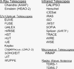
1.IntroductionParametric cost models are important tools for mission planners. They identify major architectural cost drivers, enable high-level design trades, enable cost-benefit analysis for technology development investment, and provide a basis for estimating total project cost. Unfortunately, there is no definitive model for the cost of a space telescope optical telescope assembly (OTA). The problem is that until recently there were insufficient data to generate cost models for space telescopes. This lack of data has resulted in unfounded extrapolation of ground telescope models to space telescopes and the creation of “rule of thumb” scaling laws. Typically, these cost estimating relationships (CERs) are single-variable parameter models that estimated space telescope OTA cost based on primary mirror diameter with scale factors ranging1 from 2.7 to 0.27. In the mid-1990s, after the launch of the Hubble Space Telescope (HST), Horak developed a detailed parametric cost model for space telescopes based on 17 Department of Defense (DoD) and National Aeronautics and Space Administration (NASA) missions and experimental programs.2 In 2000, Smart developed a cost model based on 13 NASA space telescopes.3 While both models are multivariable, the Horak model estimates that cost varies with diameter to the power of 0.7, while the Smart model estimates that cost varies with diameter to the power of 1.1. The NAFCOM (NASA/Air Force cost model) estimates spacecraft and launch vehicle subsystem costs based on mass as well as CERs of heritage, technology readiness, and other technical and programmatic parameters; however, it estimates space telescope cost entirely on mass. Finally, the NASA Advanced Mission Cost Model4 estimates that space telescopes cost varies with mass and difficulty level. A summary survey of all these cost models can be found in Ref. 1. In the last , several space telescopes have been developed and launched (including Kepler and Spitzer) or are under development with relatively mature cost knowledge, e.g., the James Webb Space Telescope (JWST). Thus, now there is a sufficiently detailed cost database to study CERs for space telescopes. Based on data collected from 30 different NASA, European Space Agency (ESA), and commercial space telescope missions, statistical methods are used to develop single-variable parametric space telescope OTA cost models, test published models, and establish a foundation for future multivariable parametric cost models. For the purpose of this paper, OTA is defined as the space observatory subsystem that collects electromagnetic radiation and focuses it (focal) or concentrates it (afocal). An OTA consists of the primary mirror, secondary mirror, auxiliary optics, and support structure (such as optical bench or truss structure, primary support structure, secondary support structure or spiders, etc.). An OTA does not include science instruments or spacecraft subsystems. Cost is defined as prime contract cost without any NASA labor or overhead. 2.Methodology2.1.Database CollectionThe database used in this paper consists of 30 NASA, ESA, and commercial space telescopes (Table 1). For each mission, as much data as possible was acquired about 59 different technical, programmatic and cost parameters. Sources for the database include the NAFCOM database, the RSIC (Redstone Scientific Information Center) and REDSTAR (Resource Data Storage and Retrieval System) libraries, project websites, technical papers, and interviews with mission managers, engineers and principal investigators. The Appendix0 lists the public sources, i.e., technical papers and websites, used for the database. Table 1Cost Model Missions Database.
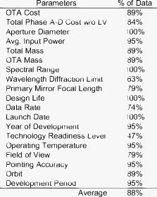
To ensure the accuracy of the database, guidelines were established for data accumulation. Each source was assigned a confidence level: For this study, data for a completed mission was assigned a confidence level of 1 to 2. And, for missions that are in-process (e.g., JWST), data can at most have a confidence level of 3. Finally, data assigned a confidence level of 4 to 5 is not included in this study.Resources such as the Scientific Instrument Cost Model (SICM) and NAFCOM are established databases used for many cost-modeling applications. As a result, they provided highly reliable cost and technical data for several different missions. The REDSTAR database is a library of cost, programmatic, and technical data on many NASA science missions. Information ranges from hand-scribed notes from the 1960s to complete project data manuals listing all relevant information for a mission. Although much of the necessary information could be found in this library, most documents required careful analysis to ensure that the information was reported at or after mission completion. With old missions such as the Copernicus Satellite (OAO-3), much of the information was not organized enough to be able to gain a complete understanding of costs. In these cases, other sources were used. REDSTAR was also not a complete resource because several of the smaller and recent missions are not yet included in the library. Data obtained directly from mission managers, principal investigators, and project engineers was given priority over other resources. These data were collected via e-mail communication, telephone conversations, and in-person interviews. With Internet websites, information was collected only from reputable and verifiable sources. Relevant information is often plentiful and easy to find online, but it is difficult to know for certain whether the data are completely accurate. As a result, the websites used most in assembling the space telescope database were from NASA, ESA, and universities. In the cases where data was found from a commercial or organizational website, a secondary source was sought to confirm the authenticity of the information. Technical papers provided a great amount of valuable data, but frequently these papers are published before the mission is completed and launched. It is very important to ensure that the data being collected are the final information. Papers published early on in a mission’s schedule are still useful in that they provide insight into how technical parameters change for increases in cost and schedule. A critical element of data collection is the importance of ensuring that definitions are consistent. For example, total mission cost is defined to be phase A-D cost, excluding launch cost. But, because different sources defined “total cost” differently, it is necessary to understand what is and is not included in the reported numbers. Similarly, different projects have different work breakdown schedule (WBS) definitions. For example, the HST included the fine guidance sensor (FGS) in their OTA WBS, while JWST does not. For the purpose of this study, we defined the FGS as part of the science and/or spacecraft instruments and not part of the OTA. Finally, we included in the database only costs that can be verified, i.e., funded contract costs. The database does not include costs associated with NASA labor (civil servant or support contractor) for program management, technical insight/oversight, or any NASA provided ground support equipment, e.g., test facilities. Because of this requirement, special care was necessary to determine the JWST cost. JWST was begun before full-cost accounting, but is now reported under full-cost accounting rules. However, the reporting guidance on how to comply with those rules has changed almost annually. Therefore, the JWST cost must be adjusted as a function of year to allow for consistent intercomparison. Consequently, because we consider only contract costs, the database underestimates the true cost to the taxpayer by at least 10% and maybe as much as 33%. 2.2.Variables StudiedFor the 30 programs listed in Table 1, data was accumulated on 59 different technical, programmatic, and cost parameters. Of these 59 parameters, 19 were selected for study as potential CERs. Table 2 lists these 19 variables and the percentage of programs for which data has been recorded for each variable. These 19 variables were selected for multiple reasons: engineering judgment of their impact on cost; their use in historical cost models, which we wish to test; and availability of the data. Cost values are represented in millions of U.S. dollars adjusted for inflation to year 2009 dollars. While data were accumulated for a wide range of telescopes, from x-ray to radio wave, this paper limits itself to 23 normal incidence UV/optical and IR telescopes. Of these 23 programs, 19 are free-flying space telescopes. The other 4 are categorized as “attached.” Three flew on the Space Shuttle Orbiter and the other is SOFIA, which flies on a Boeing 747. Table 2Cost model variables study and the completeness of data knowledge.
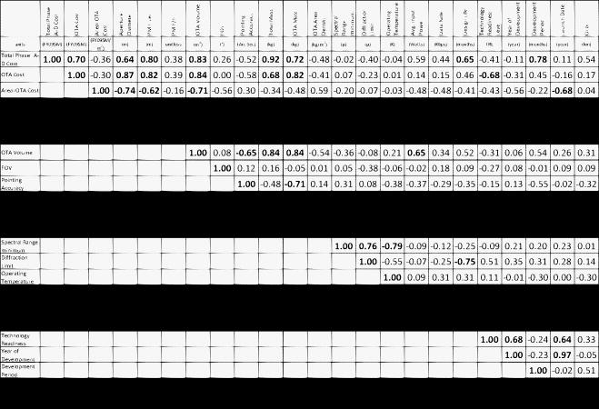
2.3.Statistical MethodsBased on experience and theory, cost is modeled by a power model with a multiplicative error term, which is appropriate for the data. To obtain a power model, ordinary least-squares regression is performed on the log-transformed variable . This operation yields an equation of the type Exponentiation gives the more familiar form:where is the independent parameter.Models are tested for “goodness of fit” via a range of statistical measures, including Pearson’s coefficient, value, and standard percent error. Pearson’s (typically denoted as just ) technically describes the percentage of variation in the actual cost that is explained by the model or simply the percentage agreement between the model and actual cost. Pearson’s is a linear space version of the more familiar log-log (used for single-variable models) or adjusted (used for multivariable models) “coefficient of linear determination” produced by log-transformed ordinary least-squares regression.5 The and are intentionally different cases, as suggested by Hu, to differentiate the two values.6 Pearson’s is used instead of log-log because it reports the percentage of variation in actual cost rather than log cost. Pearson’s is calculated by taking the square of the correlation between the actual values in the database and the values predicted by the model. The closer or is to 1.0 or 100%, the better the model. Because log-transformation is used to create models, the errors in these models must be multiplicative. If additive errors were used, estimates at the bottom of the range would be incredibly vague, while high estimates would be overly precise. For these reasons, the error was quantified using the standard percent error: where is the actual cost, is the predicted cost, is the number of data points, and is the number of estimated coefficients ( for single regression). SPE scales the residuals according to the predicted values , thus enabling meaningful comparisons of different models and construction of usable confidence intervals across the range of predictions. The SPE can be treated like any other standard deviation in making confidence intervals.6 As with any measurement of error, the lower the SPE, the better the model.After regression on any log-transformed variables, exponentiation of the model (to bring it from log-space to $-space) gives the median cost, not the mean cost. While median cost is often of more interest to cost analysts, if the mean cost is desired, one can adjust the model by a correction factor of whereis the variance of the log-space residuals.73.Cost ModelsOnce the data were verified, CERs for specific parameters were developed via the statistical parametric method of single-variable regressions. Which parameters to study were determined based on a high Pearson cross-correlation with cost, engineering judgment, and previous use in a historical cost model. 3.1.Pearson’s Cross-Correlation Analysis of ParametersThe first step in developing a cost model is to perform a Pearson's cross-correlation analysis to determine the statistical correlation between any two parameters (Figure 1). Parameters with a high statistical correlation with cost are identified as CERs. Cross-correlation analysis is important because it isolates key cost model CERs, identifies linkages between CERs and verifies that correlations and their “signs” are consistent with engineering judgment. Additionally, it serves as the foundation for a future multivariable cost model. Each cell in the cross-correlation matrix consists of the Pearson's correlation coefficient between the entry's row label data and column label data. In our case, the parameters studied are all log-transformed. This means that a correlation coefficient close to 1.0 implies a strong power relationship (i.e. parameter is proportional to some power of parameter ), instead of a strong linear one, as is the case with raw parameters. However high correlation does not imply a causal effect; both parameters might be dependent upon a third known or unknown parameter. Because of such linkages, care must be taken when performing multivariable fitting of data to independent variables that are strongly correlated with one another. This situation can lead to the well-known problem of multicollinearity. One indication of multicolinearity is coefficients with non intuitive or “wrong” signs. There are several methods for dealing with this issue, including only incorporating one of the correlated variables or combining these variables via a collector variable. In this study, we have defined four collector variables: Primary Mirror /# (focal length/diameter), OTA Volume (focal length × area), OTA Areal Density (mass/area) and OTA Areal Cost (cost/area). Figure 1 shows the cross-correlation matrix for the 19 parameters in our study. CERs with the most significant statistical correlation to OTA cost are primary mirror diameter (87%), OTA mass (82%) and primary mirror focal length (82%). Another potential CER is TRL (technology readiness level) . While its correlation coefficient is not as large as for diameter, its sign is in the direction of engineering judgment. Its negative sign indicates that the higher the initial TRL of the OTA technology the lower the OTA cost. Similarly, the CER with the most significant statistical correlation to Total Cost is Total Mass (92%). Some interesting parameter correlations which identify relationships consistent with engineering judgment are OTA mass with pointing accuracy and spectral range with operating temperature . However, as noted above, just because a parameter has a high correlation with cost does not make it a CER. This is because parameters can be linked with each other via engineering principles or programmatic logic. For example, a strong statistical correlation can be explained by sound engineering principles between diffraction limited wavelength and operating temperature: infrared telescopes are generally cryogenic while visible telescopes typically operate above 280K. Similarly, there are solid engineering principles to explain the correlation between OTA mass and primary mirror diameter: bigger mirrors with their support structure tend to have more mass than smaller mirrors. Another example of highly correlated variables is total mass and OTA mass. For the purpose of developing a single variable parametric cost model, we will constrain ourselves to the two most significant parameters: primary mirror diameter and mass. However, as will be shown below, none of the single variable models developed in this paper can perfectly predict space telescope cost. Therefore, eventually a multivariable model is required. Specific variables to be considered for future multivariable analysis will be selected based upon the cross-correlation matrix. And, a careful study of the matrix easily identifies potential candidate CERs such as power, TRL, year of launch, design life or period of development. Interestingly, other parameters frequently assumed to be cost drivers, such as wavelength or operating temperature, do not seems to be highly correlated with cost. 3.2.OTA Cost versus Total CostThe next question is whether to model OTA cost or total cost. Engineering judgment says that OTA cost is most closely related to OTA engineering parameters. However, managers and mission planners are really more interested in total phase A-D cost. For this study, total cost is defined as all mission contract costs excluding government costs, launch costs, mission operations, and data analysis. Analysis of the 14 free-flying missions (for which we have both OTA and total cost) indicates that there is a linear relationship between OTA cost and total cost [Fig. 2]. OTA cost is of phase A-D total cost with a model residual standard deviation of approximately $300M. Note that we did not include attached telescopes in this analysis because their total costs do not include a spacecraft. Fig. 2Relationship between OTA cost and total cost: (a) OTA cost versus total with Chandra and (b) OTA cost normalized by total cost. 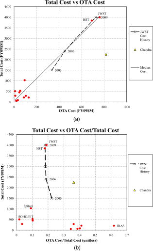 From the graph, it is clear that HST and JWST are strong influences on this relationship and might be overweighted in the fit. Therefore, throughout this paper we use two methods to test our results. The first is to compare the results with Chandra (another expensive flagship class mission). The second method is to normalize the data. As shown in Fig. 2, the comparison with Chandra is not good; however, based on sound engineering principles, this is explainable. Unlike HST and JWST, Chandra has a very simple scientific instrument suite and spacecraft. Therefore, the telescope is a significantly larger percentage of the total mission cost. Also, because Chandra is a grazing angle of incidence telescope, the fabrication cost for its diameter is much higher than if it were a normal incidence telescope. A more interesting result is provided by normalizing the OTA cost by the total mission cost. Figure 2 shows that while the OTA cost tends to be close to 20% for large missions, the OTA cost for small missions varies widely from a low of 2% for the SOHO/EIT instrument OTA (Solar & Heliospheric Observatory Extreme-Ultraviolet Imaging Telescope) to a high of 62% for IRAS (Infrared Astronomical Satellite). The SOHO/EIT result is easy to explain, the EIT was just one of many different SOHO instruments. The average of the normalized OTA cost in Figure 2 is . And, if SOHO/EIT and IRAS are excluded, the average is still . Another normalization analysis was performed by developing a generic WBS that represents the allocation between various cost elements for an “average” mission. Of the 14 free-flying missions with both total mission cost and OTA cost data, we have sufficiently detailed WBS data to do this analysis for 7 missions: GALEX, HST, IRAS, IUE, JWST, Kepler, and Spitzer. The WBS for each of these 7 missions was mapped into a common WBS. Then the percentage of each WBS element as a function of total cost was calculated and averaged to produce a generic cost allocation. This analysis indicates that the OTA cost is approximately 30% of the total mission cost (Fig. 3). The 20 or 25 or 30% scale factor found in this study is consistent with both the PRC8 and Horak 2, 9 models discussed in Ref. 1. If one defines total payload cost as the sum of design and development, and flight unit manufacturing cost, the PRC model predicts that the cost of the flight unit is 20 to 25% of the total cost. And, if one assumes that the flight unit quantity is one (which is often the case for NASA telescopes) and that there is both an engineering and qualification unit; then, the Horak model predicts that the flight unit cost is 33% of the total design cost and 25% of the total mission cost. Given the linear relationship between total cost and OTA cost, and given the intuitive (as well as statistical) correlation between OTA cost and OTA engineering parameters, this paper chooses to derive cost estimating relationships for OTA cost. However, this approach does ignore variables such as average power and design life, which have a high correlation with total cost and a small correlation with OTA cost. Such variables influence spacecraft and instrument costs with a minimal impact on OTA cost. 3.3.Single-Variable Cost ModelsOTA CERs were examined for aperture diameter, mass, primary mirror focal length, -number, average power, data rate, design life, and wavelength. Of these, we chose to study aperture diameter and mass as single variable model CERs. Variables such as focal length, power, wavelength, operating temperature, and design life will be considered as secondary variables in a future multivariable analysis. The choice of diameter and mass for analysis is consistent with common practice. Historically, ground-based telescope and space telescope models developed by astronomers and optical engineers estimate cost as a function of primary mirror diameter. Also, models developed by aerospace engineers and cost modelers typically estimate cost as a function of mass. However, as discussed in Stahl,1 care should be taken when considering a mass only model, because mass is really an indicator of other parameters such as volume, stiffness or complexity. For each of the two models developed, we considered two cases: with and without JWST. Given that it is currently under development, including JWST in the analysis is both relevant and risky. Including JWST is relevant because it represents a new paradigm for space telescopes, i.e., segmented and deployed on orbit. As a result, it is the most complex and technologically advanced telescope ever built. Therefore, it is interesting to compare JWST’s cost with historical costs. Including JWST in the cost analysis is risky because it is not a completed mission and its cost may increase further. Both JWST’s OTA and total mission costs have increased by over 100% since the start of phase A in 2003. This cost growth is represented in all appropriate figures as a line with discrete cost data points representing the 2003 phase A/B cost estimate, the 2006 “replan” cost estimate and the 2009 phase C/D cost estimate. The risk of including JWST is mitigated by a sensitivity analysis of the cost models, which indicates that changing the JWST total mission cost by has only a slight effect on the independent variable power term. The bigger effect is to increase or decrease . 3.3.1.Cost as a function of aperture diameter CERBased on a sample size of 16 free-flying space telescopes (excluding JWST), a single-variable cost estimating relationship was developed for OTA cost as a function of primary mirror diameter (Fig. 4) As indicated by Pearson’s , diameter is a good predictor of OTA cost. For this regression, diameter explains 84% of the OTA cost variation. The reason for the good fit is simple. It is easy to draw a straight line between two data points, i.e., HST and all the small telescopes. But, as indicated by SPE, there is a large statistical error. If the 2009 JWST cost is added to the regression, then the CER isAs shown in Fig. 4, the JWST OTA cost is smaller than that of HST. Thus, including JWST in the regression causes the diameter power term to decrease slightly. Also, because we now have two large missions with differing costs, the fit (as indicated by Pearson’s ) is not as “good.” Interestingly, the noisiness of the fit remains unchanged. Possible explanations for the cost difference between HST and JWST might be that the JWST OTA is being manufactured according to a new paradigm, which reduces its areal cost (cost per unit area of collecting area), or there are engineering differences between the two which drive cost, or that JWST is not yet complete and its OTA cost may increase further. To illustrate the impact of using an early cost estimate, if the regression is performed based upon the 2006 JWST “replan” cost, the CER isBased on Pearson’s one might conclude that the 2006 JWST OTA cost estimate was obviously inconsistent with history. However, if one is asserting that JWST is being built according to a new cost paradigm, then the value would have actually supported that hypothesis. The authors will leave it to the reader to draw their own conclusion about the probable final JWST OTA cost based on Fig. 4. For the balance of this paper, we will use only the 2009 JWST cost.Fig. 4OTA cost versus aperture diameter scaling law for 17 free-flying UV/OIR systems (including 2009 JWST). Plot includes 90% confidence and prediction intervals, and data points. Chandra data point is not included in the regression. 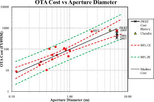 Regarding potential concern about HST and JWST overweighting the cost versus aperture diameter fit, we both plot the cost of Chandra and perform a separate area weight normalization analysis. For this and all future figures, we plot the cost of Chandra as a -diameter normal incidence mirror, which has the same surface area as the four nested shell grazing angle of incidence -diameter x-ray mirror. Also, while this Chandra data point may be interesting, it is not necessarily applicable. Even though the Chandra equivalent cost appears to be “in-family,” caution is required because Chandra is an x-ray telescope and does not have a normal incidence telescope support system. If the Chandra data point were for a mirror, it would be significantly above the trend line. The better sanity test is to normalize OTA cost by area (Fig. 5): For these regressions, the sign of the mirror diameter exponent is consistent with expectation. But, the quality of the fit, as indicated by value, is not as good. Only half of the variation in OTA areal cost can be attributed to the primary mirror diameter. By eliminating the strong first-order diameter influence, we expose data spread associated with second-order factors such as diffraction-limited wavelength or operational temperature or technology maturity etc. This analysis will serve as a point of departure for a future multivariable parametric cost model. An indication of how areal cost normalization impacts cost versus mirror diameter is the fact that removing JWST from the regression has a negligible effect on the result.Fig. 5OTA areal cost versus aperture diameter scaling law for 17 free-flying UV/OIR systems (including 2009 JWST). Plot includes 90% confidence and prediction intervals, and data points. Chandra data point is not included in the regression. 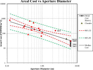 Of all the historical cost models, the cost versus diameter result is closest to the 2000 Smart model,3 which, while a multivariable model, estimates cost to vary with primary mirror diameter to the power of 1.12. The next closest historical model is the Bely model,10 which, while also a multivariable model, estimates cost to vary with diameter to the power of 1.6. Furthermore, the preceding result is clearly different from any model, which suggests that space telescope costs scale with aperture to the power of 2.0 to 2.8 (Ref. 1); a fact that is reenforced by Fig. 5, which shows that areal cost (cost per square meter) decreases with increasing collecting aperture diameter. Larger telescopes collect more photons at a lower cost per photon and with better resolution than smaller telescopes. Therefore, larger telescopes provide a higher return on investment as well as better science. 3.3.2.Cost as a function of massWhile for astrophysicists, telescope aperture diameter is the single most important parameter because it drives system level observatory performance. For engineers and mission planners, mass (and volume) is of equal if not greater importance. Total system mass determines what vehicle can or cannot be used to launch the payload. Significant engineering costs are expended to keep a given payload inside of its allocated mass budget. Therefore, from a mission perspective, space telescopes are really designed to mass. While developing the mass CER, an interesting (and possibly obvious) cost versus mass relationship was identified. It costs more to make a lightweight telescope than it costs to make a heavy telescope. Of the 23 mission in the database, there are 19 free-flying telescopes (15 for which we have OTA cost data) and 4 that are attached (3 to the Space Shuttle Orbiter and SOFIA to a Boeing 747 airplane). Obviously, we cannot compare total mission costs of attached missions with those of free-fliers because the Orbiter or 747 replaces the spacecraft costs. But, the OTA cost comparison should be valid. As shown in Fig. 6, the 4 “attached” missions’ OTA costs are approximately 60% less than the free-flying missions’ OTA costs. Also, the attached missions’ OTA mass is approximately larger than the free-flier missions’ OTA mass. The story gets better when the data is analyzed as a function of aperture diameter. For a given aperture diameter, attached OTAs are 1.5 to 4× more massive and 33% to 66% less expensive than free-flying OTAs. On average it appears, that for a given aperture diameter, increasing OTA mass by 2× might reduce cost by 2×. One explanation is that “attached” telescopes do not have the same mass and volume design constraints as free-flying telescopes. Therefore, their designers have the luxury to “trade” extra mass for a simpler, more robust, higher TRL, less complex design. As discussed by Beardon11, 12 and quantified in NASA’s own parametric cost model,4 less complex or less difficult designs cost less than more complex or more difficult designs. Fig. 6OTA cost versus OTA mass for free-flying UV/OIR space telescopes (including 2009 JWST) and attached telescopes. Plot includes 90% confidence and prediction intervals, and data points. Chandra data point is not included in the regression. 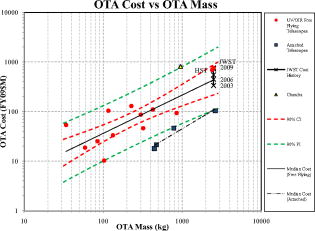 Based on a sample size of 15 free-flying space telescopes, a single variable cost estimating relationship was developed for OTA cost as a function of OTA mass: It is interesting to observe that this result is close to the 0.65 coefficient of the NASA mass-based cost model.4 If one considers only the value, one might be tempted to assert that mass is the most important parameter driving OTA cost given that it can explain 92% of the cost variation. Or, that all one needs to know to predict an OTA cost is its mass budget. However, the SPE as well as common sense indicate otherwise. The cost versus mass model SPE is very noisy—even noisier than the cost versus diameter models. Also, as already discussed, our analysis shows that, for a given aperture diameter, attached OTAs which are ~2× more massive than free-flying OTAs are ~50% less expensive. Finally, there is the lead brick analogy, i.e., common sense says that it must be more expensive to launch a very complex JWST than to launch a lead brick with the same mass.Note also that HST and JWST have virtually identical OTA masses and costs (Fig. 6). It is impossible to say why HST and JWST have virtually identical masses and costs given their dramatic architectural differences. One explanation is that architectural differences do not matter. That it really is all about the mass. But then, consider Chandra. Its OTA is 20% less massive but has the same cost. And the Chandra OTA architecture is even more different. As an x-ray telescope, it is four pairs of nested solid glass cylindrical shells. So, maybe a potential explanation is that this is the maximum amount that can be spent on a flagship mission OTA and that the OTA is designed to cost. Next, analysis was performed to examine total payload cost as a function of total payload mass. The reason is because some have argued that: while mass may not be an appropriate CER for OTA cost, it may be a good CER for total mission cost because total mission mass includes spacecraft and science instruments. Using 15 free-flying space telescopes, a CER was developed for total phase A-D cost as a function of total mass (Fig. 7): Again, considering only the value, one might be tempted to assert that mass is the most important parameter driving total mission cost. But again, the fit is noisy, although not as noisy as any of the other models.Fig. 7Total cost versus total mass scaling law for free-flying UV/OIR space telescopes (including 2009 JWST). Plot includes 90% confidence and prediction intervals, and data points. Chandra data point is not included in the regression. 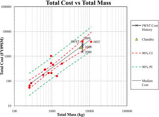 Note that, while the total cost for both HST and Chandra are on the Fig. 7 trend line—which might support a supposition that mass is a good CER—the total cost for JWST is not. Early in the program, JWST total cost was below the trend line—which would have reenforced the optimistic view that JWST was being designed to a new paradigm which “broke” the traditional cost curve. But now, JWST total cost is above the trend line—which argues that mass really is not a good predictor of total cost. One explanation for these facts is the launch vehicle mass constraint. HST and Chandra were both launched via the Space Shuttle. Therefore, they were designed to similar mass constraints. However, JWST is being launch by an Ariane 5 rocket, which constrains JWST’s total mass to the total mass of HST. Consequently, the JWST program is incurring significant cost as it works through the engineering challenges of packaging a -aperture telescope into a volume- and mass-constrained launch vehicle. In other words, JWST is more complex than HST. Again, maybe mass is not a true driver for cost but rather is an indicator of one or more true drivers, which are difficult to quantify. And, maybe the best way to reduce cost for large space telescopes is to develop cost-effective heavy lift launch vehicles with lower mass to orbit costs and larger total payload volumes. Finally, in our database, the average mission total mass is approximately that of the average OTA mass (with a statistical correlation of 0.92). This is interesting because, as discussed in Sec. 3.2, total cost was found to be 3.3 to OTA cost. Also interesting is the fact that none of the three flagship missions are average. Because JWST is highly mass constrained, its allocated total mass is only its OTA mass allocation. While HST and Chandra, which were launched by the Space Shuttle, have ratios of and , respectively. Note that in the case of Chandra, we are excluding the mass of the upper inertial stage. Also, its mass ratio is probably high because it is an x-ray telescope, and x-ray science instruments are typically massive. Regarding the cost ratios, JWST’s projected total cost is its projected OTA cost, while HST was and Chandra was . In this case, the low Chandra cost ratio is probably because it is an x-ray telescope. The JWST and HST cost ratios are probably similar because they are both normal incidence flagship class observatories. While statistically mass may appear to be a good single-variable CER, it is not an independent variable. Mass is actually a dependent variable. It is a surrogate for other parameters which are driven by science requirements. For example, the larger the telescope aperture, the larger the telescope structure needed to support it. Also, a larger telescope aperture probably means more and larger science instruments which have more mass. These science instruments require a more capable spacecraft and both require a larger electrical power system. Reviewing the correlation matrix shown in Fig. 1, OTA mass is highly correlated with primary mirror diameter, primary mirror focal length, and the volume collecting variable. This is consistent with engineering judgment, which indicates that the greater a telescope’s volume, the larger should be its mass. It has a weaker correlation with pointing accuracy and average power. Engineering judgment might also support pointing accuracy, such that the more precisely a telescope must point, the stiffer the telescope structure must be, and thus, the more mass the telescope must have. One could also argue that a mission that uses a lot of power has more science instruments than a mission that does not use very much power. Total mass has similar correlations except that design life is more strongly correlated than either pointing accuracy or average power. This might be because design life is driven by system redundancies, which have a multiplier effect on mass. Exploration of the linkages between mass and various engineering parameters requires a multivariable analysis. 4.ConclusionCost models have several uses. They identify major architectural cost drivers and allow high-level design trades. They enable cost-benefit analysis for technology development investment. They also provide a basis for estimating total project cost. This paper is part of a larger effort to develop a multivariable parametric cost model for space telescopes. Cost and engineering parametric data were collected on 23 different NASA, ESA, and commercial space telescopes. Statistical correlations were evaluated between 19 of 59 variables sampled. Four single-variable CERs were developed for OTA cost and total mission cost as a function of OTA diameter, OTA mass, and total mission mass (Table 3). Table 3Summary of single-variable cost model statistics.
When reviewing Table 3, the exponent is the power to which the variable is raised; the coefficient is the multiplier; is the standard deviation of the residual in log space; Pearson’s is the percentage of agreement between the actual cost and the model; SPE is the percentage error of the regression; and is the number of elements in the data set regression. In general, one wants Pearson’s to be close to 1 and and SPE to be close to 0. OTA mass has the highest Pearson’s for OTA cost, but it also has the highest SPE. Total mass appears to be statistically a good indicator of total mission cost. In general, however, mass should be avoided as a CER because it is a secondary indicator of other parameters and because many missions are designed to a mass-budget defined by launch vehicle constraints, thereby resulting in a more complex and thus more expensive mission architecture. As discussed in Sec. 3.3.2. for a given aperture diameter, OTAs that are ~ more massive are ~50% less expensive. Therefore, maybe the best way to reduce future large-aperture space telescopes is to develop cost-effective heavy lift launch vehicles that will enable mission planners to trade complexity for mass. From both an engineering and a science perspective, aperture diameter is the best parameter on which to build a space telescope cost model. Aperture defines the observatory’s science performance and determines the payload’s size and mass. While the results are consistent with some historical cost models, our results invalidate long-held “intuitions,” which are often purported to be “common knowledge.”11 Space telescope costs vary almost linearly with diameter and not to a power of or or even . But, diameter by itself only explains of the OTA cost variation and only of the OTA areal cost variation. Therefore, other factors must influence cost. The next step is to develop a multivariable cost model using multivariable regression techniques. Finally, we would like to make three disclaimers. First, the results of this study are only as good as the data, and given the lack of large-aperture space telescopes, we really need a complete cost WBS for the Herschel space telescope. Second, this study cannot and will not be able to determine other cost impacts of mirror diameter such as the industrial infrastructure necessary to make large mirrors. Third, half as a joke and half as a true statement, maybe the best possible CER for space telescopes is the number of pages of documentation produced by the project (either kilograms of paper or terabytes of data). But in reality, this is a trailing indicator instead of a leading indicator. AppendicesAppendixThe following sources were used in compiling the space telescope cost model database:
ReferencesH. P. Stahl,
“Survey of cost models for space telescopes,”
Opt. Eng., 49
(5), 053005
(2010). https://doi.org/10.1117/1.3430603 0091-3286 Google Scholar
J. A. Horak, C. J. Brown, L. M. Giegerich, and W. E. Waller,
“Strategic and experimental IR sensor cost model II,”
(1993) Google Scholar
C. B. Smart,
“Telescope cost estimating relationship,”
(2000) Google Scholar
S. A. Book, and P. H. Young,
“The trouble with ,”
Int. Soc. Param. Anal. J. Param., XXV
(1), 87
–112
(2006). Google Scholar
S.-P. Hu,
“ vs. ,”
3
–7
(2008). Google Scholar
G. L. Baskerville,
“Use of logarithmic regression in the estimation of plant biomass,”
Canad. J. Forest Res., 2 49
–53
(1972). https://doi.org/10.1139/x72-009 Google Scholar
. “Cost estimating relationships for spaceborne telescopes,”
(1985) Google Scholar
J. A. Horak, C. J. Brown, and W. E. Waller,
“Strategic and experimental IR sensor cost model II,”
(1994) Google Scholar
P. Y. Bely, The Design and Construction of Large Optical Telescopes, Springer-Verlag, New York
(2003). Google Scholar
D. Bearden,
“Perspectives on NASA mission cost and schedule performance trends,”
(2008). Google Scholar
D. A. Bearden,
“A complexity-based risk assessment of low-cost planetary missions: when is a mission too fast and too cheap?,”
(2000). Google Scholar
Biography
|
|||||||||||||||||||||||||||||||||||||||||||||||||||||||||||||||||||||||||||||||||||||