Particle probability hypothesis density filtering for multitarget visual tracking with robust state extraction

Jingjing Wu; Shiqiang Hu; Yang Wang

doi:10.1117/1.3638121

1 September 2011 Particle probability hypothesis density filtering for multitarget visual tracking with robust state extraction

Jingjing Wu, Shiqiang Hu, Yang Wang

Author Affiliations +

Optical Engineering, Vol. 50, Issue 9, 090502 (September 2011). https://doi.org/10.1117/1.3638121

Abstract

Particle probability hypothesis density (PHD) filter-based visual trackers have achieved considerable success in the visual tracking field. But position measurements based on detection may not have enough ability to discriminate an object from clutter, and accurate state extraction cannot be obtained in the original PHD filtering framework, especially when targets can appear, disappear, merge, or split at any time. To meet the limitations, the proposed algorithm combines a color histogram of a target and the temporal dynamics in a unifying framework and a Gaussian mixture model clustering method for efficient state extraction is designed. The proposed tracker can improve the accuracy of state estimation in tracking a variable number of objects.

1. Introduction

Probability hypothesis density (PHD) filter-based¹ trackers have enjoyed growing popularity in recent years, particularly in the field of nonlinear non-Gaussian multitarget visual tracking. The original PHD filter-based visual tracker usually uses outputs of detectors, such as a motion detector to establish the observation model, whose efficiency relies on the accuracy of the detection.² In addition, due to the potential nonlinearity and non-Gaussianity of target models in most visual trackers, a particle PHD filter³ is used to implement the PHD recursion. However, the intersections of multiple targets like occlusion and clutter often lead to the complex multimodality distribution of the resampled particles, which obviously increase the complexity of state extraction. The classical k-means clustering algorithm may present serious degradation in state extraction performance.

In this paper, to avoid inaccurate detection generating estimation errors in the original PHD filter-based visual tracker,² color histogram with position constraints⁴ is incorporated into the PHD filtering framework, which combines the appearance model of the target with its temporal dynamics in a unifying framework. Moreover, to obtain more accurate state estimates, a new state extraction method based on Gaussian mixture model (GMM) clustering is proposed. Hence, a robust visual tracking framework is obtained.

The multitarget visual tracking problem can be formulated as multitarget Bayes filter in a random finite set (RFS) framework by propagating the multiple-target posterior in time. The particle PHD filter³ is a sequential Monte Carlo implementation for the multitarget Bayes filter, which approximates the PHD with a set of random samples (weighted particles). The particle PHD filter involves prediction and update steps. Let posterior PHD at time k − 1 be approximated by [TeX:] $\{ w_{k - 1}^{(i)},x_{k - 1}^{(i)} \} _{i = 1}^{L_{k - 1} }$ ${w_{k - 1}^{(i)}, x_{k - 1}^{(i)}}_{i = 1}^{L_{k - 1}}$ of L_{k − 1} particles and their corresponding weights. The predicted PHD v_{k|k − 1}(x_k) can be approximated by [TeX:] $\{ \tilde w_{k|k - 1}^{(i)},\tilde x_k^{(i)} \} _{i = 1}^{L_{k - 1} + J_k }$ ${{\tilde{w}}_{k | k - 1}^{(i)}, {\tilde{x}}_{k}^{(i)}}_{i = 1}^{L_{k - 1} + J_{k}}$ after applying importance sampling below

Eq. 1

[TeX:] \documentclass[12pt]{minimal}\begin{document}\begin{equation} v_{k|k - 1} (x_k) = \sum\limits_{i = 1}^{L_{k - 1} + J_k } {\tilde w_{k|k - 1}^{(i)} \delta _{\tilde x_k^{(i)} } } (x_k), \end{equation}\end{document}

v_{k | k - 1} (x_{k}) = \sum_{i = 1}^{L_{k - 1} + J_{k}} {\tilde{w}}_{k | k - 1}^{(i)} δ_{{\tilde{x}}_{k}^{(i)}} (x_{k}),

where

Eq. 2

[TeX:] \documentclass[12pt]{minimal}\begin{document}\begin{eqnarray} \displaystyle\tilde w_{_{k|k - 1} }^{(i)} = \! \left\{ {\begin{array}{*{20}c} {\displaystyle\frac{{\phi _{k|k - 1} \big(\tilde x_k^{(i)},x_{k - 1}^{(i)} \big)w_{k - 1}^{(i)} }}{{q_k \big(\tilde x_k^{(i)} |x_{k - 1}^{(i)},Z_k \big)}},} & {i = 1, \cdots,L_{k - 1} } \\ [-4pt] \\ {\displaystyle\frac{{\gamma _k \big(\tilde x_k^{(i)}\big)}}{{J_k p_k \big(\tilde x_k^{(i)} |Z_k \big)}}{\rm,}} & \!\!\!\!\!\!{i \!=\! L_{k - 1} \!+ \! 1, \cdots,L_{k - 1} \!+ \! J_k } \\ \end{array}} \right.\!\!\!.\hspace{-10pt}\nonumber\\ \end{eqnarray}\end{document}

\begin{matrix} {\tilde{w}}_{k | k - 1}^{(i)} = \{\begin{matrix} \frac{φ_{k | k - 1} ({\tilde{x}}_{k}^{(i)}, x_{k - 1}^{(i)}) w_{k - 1}^{(i)}}{q_{k} ({\tilde{x}}_{k}^{(i)} | x_{k - 1}^{(i)}, Z_{k})}, & i = 1, \dots, L_{k - 1} \\ \frac{γ_{k} ({\tilde{x}}_{k}^{(i)})}{J_{k} p_{k} ({\tilde{x}}_{k}^{(i)} | Z_{k})}, & i = L_{k - 1} + 1, \dots, L_{k - 1} + J_{k} \end{matrix} . \end{matrix}

Here, [TeX:] $q_k ( \cdot |x_{k - 1}^{(i)},Z_k)$

q_{k} (\cdot | x_{k - 1}^{(i)}, Z_{k})

and p_k( · |Z_k) are the importance functions for targets at time k − 1 and new targets at time k, ϕ_{k|k − 1}( ·, ·) denotes the intensity of survived and spawned targets from time k − 1, and γ_k( · ) is the intensity of new target birth RFS. Once the observation likelihood [TeX:] $p(z_k |\tilde x_k^{(i)})$

p (z_{k} | {\tilde{x}}_{k}^{(i)})

is obtained, the weights in Eq. 2 are updated by

Eq. 3

[TeX:] \documentclass[12pt]{minimal}\begin{document}\begin{equation} \tilde w_k^{(i)} = \left[ {P_M (\tilde x^{(i)}) + \sum\limits_{z_k \in Z_k } {\frac{{P_D \big(\tilde x_k^{(i)} \big) P \big(z_k |\tilde x_k^{(i)} \big)}}{{\kappa _k (z) + C_k (z)}}} } \right]\tilde w_{_{k|k - 1} }^{(i)}, \end{equation}\end{document}

{\tilde{w}}_{k}^{(i)} = [P_{M} ({\tilde{x}}^{(i)}) + \sum_{z_{k} \in Z_{k}} \frac{P_{D} ({\tilde{x}}_{k}^{(i)}) P (z_{k} | {\tilde{x}}_{k}^{(i)})}{κ_{k} (z) + C_{k} (z)}] {\tilde{w}}_{k | k - 1}^{(i)},

where [TeX:] $P_M (\tilde x^{(i)}) = 1 - P_D (\tilde x^{(i)})$

P_{M} ({\tilde{x}}^{(i)}) = 1 - P_{D} ({\tilde{x}}^{(i)})

with [TeX:] $P_D (\tilde x^{(i)})$

P_{D} ({\tilde{x}}^{(i)})

denoting the detection probability, κ_k( · ) is the clutter intensity, and [TeX:] $C_k (z) \break = \sum\nolimits_{j = 1}^{L_{k - 1} + J_k } {P_D (\tilde x_k^{(j)})P_k (z_k |\tilde x_k^{(j)})w_{_{k|k - 1} }^{(j)} }$

C_{k} (z) = \sum_{j = 1}^{L_{k - 1} + J_{k}} P_{D} ({\tilde{x}}_{k}^{(j)}) P_{k} (z_{k} | {\tilde{x}}_{k}^{(j)}) w_{k | k - 1}^{(j)}

.

2. Tracking Model

In the proposed tracker, the target candidate in an image is approximated with a w × h rectangle. Let the state of a target at time k be [TeX:] $x_k = (p_{x,k},\dot p_{x,k},p_{y,k},\dot p_{y,k},w,h)^T$ $x_{k} = {(p_{x, k}, {\dot{p}}_{x, k}, p_{y, k}, {\dot{p}}_{y, k}, w, h)}^{T}$ with the centriod p_k = (p_{x, k}, p_{y, k}) and the target speed. Assume that each target follows a linear Gaussian constant velocity model, i.e.,

Eq. 4

[TeX:] \documentclass[12pt]{minimal}\begin{document}\begin{equation} x_k = {\bf F}x_{k - 1} + v_k, \end{equation}\end{document}

x_{k} = F x_{k - 1} + v_{k},

where F is the state, transition matrix and v_k is the zero-mean Gaussian white process noise.

To incorporate the appearance model into the tracking framework, we design the observation model by a color histogram.⁴ Let [TeX:] $\{ {\bf s}_i \} _{{i}= 1 \cdots {n _{h }}}$ ${s_{i}}_{i = 1 \dots n_{h}}$ be the pixel locations of the target centered at p_k = (p_{x, k}, p_{y, k}), and the window radius be h = (w, h). Define a function [TeX:] ${\mathop{\rm b}\nolimits}:R^2 \to \{ 1 \cdots m\}$ $b : R^{2} \to {1 \dots m}$ associating the pixel at location s_i to the index [TeX:] ${\mathop{\rm b}\nolimits} ({\bf s}_i)$ $b (s_{i})$ of the histogram bin corresponding to the color of that pixel. The color histogram of a target candidate [TeX:] ${\bf \hat q}({\bf p}_k)$ $\hat{q} (p_{k})$ and the probability of the feature u = 1, ⋅⋅⋅, m are defined by Eqs. 5, 6,

Eq. 5

[TeX:] \documentclass[12pt]{minimal}\begin{document}\begin{equation} {\bf \hat q}({\bf p}_k) = \{ \hat q^{(u)} ({\bf p}_k)\} _{u = 1, \cdots,m},\sum\limits_{u = 1}^m {\hat q^{(u)} ({\bf p}_k)} = 1, \end{equation}\end{document}

\hat{q} (p_{k}) = {{\hat{q}}^{(u)} (p_{k})}_{u = 1, \dots, m}, \sum_{u = 1}^{m} {\hat{q}}^{(u)} (p_{k}) = 1,

Eq. 6

[TeX:] \documentclass[12pt]{minimal}\begin{document}\begin{equation} \hat q^{(u)} ({\bf p}_k) = C_h \sum\limits_{i = 1}^{n_h } {\mathop{\rm k}\nolimits} \left(\left\| {\frac{{{\bf p}_k - {\bf s}_i }}{{\bf h}}} \right\|\right)\delta [{\mathop{b}\nolimits} ({\bf s}_i) - u], \end{equation}\end{document}

{\hat{q}}^{(u)} (p_{k}) = C_{h} \sum_{i = 1}^{n_{h}} k (‖\frac{p_{k} - s_{i}}{h}‖) δ [b (s_{i}) - u],

where u denotes the color histogram bins, k is a spatially weighting function and C_h is a normalization term. Similarly, the reference target model can be represented by [TeX:] ${\bf \hat q}_c \break = \{ \hat q_c^{(u)} \} _{u = 1, \cdots,m}$

{\hat{q}}_{c} = {{\hat{q}}_{c}^{(u)}}_{u = 1, \dots, m}

. Then the observation likelihood is defined by the similarity between a target candidate [TeX:] ${\bf \hat q}({\bf p}_k)$

\hat{q} (p_{k})

and the reference target model [TeX:] ${\bf \hat q}_c $

{\hat{q}}_{c}

, i.e.,

Eq. 7

[TeX:] \documentclass[12pt]{minimal}\begin{document}\begin{equation} p(z_k |x_k) = \frac{1}{{\sqrt {2\pi } \sigma _c }}\exp \left\{ { - \frac{{d^2 ({\bf \hat q}({\bf p}_k),{\bf \hat q}_c)}}{{2\sigma _c^2 }}} \right\}, \end{equation}\end{document}

p (z_{k} | x_{k}) = \frac{1}{\sqrt{2 π} σ_{c}} \exp \{- \frac{d^{2} (\hat{q} (p_{k}), {\hat{q}}_{c})}{2 σ_{c}^{2}}\},

where [TeX:] $d({\bf \hat q}({\bf p}_k),{\bf \hat q}_c) = \sqrt {1 - \rho [{\bf \hat q}({\bf p}_k),{\bf \hat q}_c]} $

d (\hat{q} (p_{k}), {\hat{q}}_{c}) = \sqrt{1 - ρ [\hat{q} (p_{k}), {\hat{q}}_{c}]}

is the similarity computed by Bhattacharyya coefficient [TeX:] $\rho [{\bf \hat q}({\bf p}_k),{\bf \hat q}_c] \break = \sum\nolimits_{u = 1}^m {\hat q^{(u)} ({\bf p}_k)\hat q_c^{(u)} } $

ρ [\hat{q} (p_{k}), {\hat{q}}_{c}] = \sum_{u = 1}^{m} {\hat{q}}^{(u)} (p_{k}) {\hat{q}}_{c}^{(u)}

, and σ_c is the standard deviation of noise which is determined experimentally.

3. GMM Clustering

In the particle PHD filter, a clustering algorithm is required to detect the peaks of the PHD defining candidate states of targets from the resampled particles. We propose a GMM clustering method for state extraction. First, GMM is used to fit the underlying distribution of a resampled particle x_k as

Eq. 8

[TeX:] \documentclass[12pt]{minimal}\begin{document}\begin{equation} S_k (x_k |\Theta _k) = \sum\limits_{l = 1}^{G_k } {\pi _k^l } {\cal N} \big(x_k |\mu _k^l,\Sigma _k^l \big){\rm with }\sum\limits_{l = 1}^{G_k } {\pi _k^l = 1}, \end{equation}\end{document}

S_{k} (x_{k} | Θ_{k}) = \sum_{l = 1}^{G_{k}} π_{k}^{l} N (x_{k} | μ_{k}^{l}, Σ_{k}^{l}) with \sum_{l = 1}^{G_{k}} π_{k}^{l} = 1,

where G_k is the number of Gaussian components, and [TeX:] $\Theta _k = \{ \pi _k^l,\mu _k^l,\Sigma _k^l \}$

Θ_{k} = {π_{k}^{l}, μ_{k}^{l}, Σ_{k}^{l}}

with weight, mean, and covariance is the parameter set of a Gaussian item. Assume that the state vectors of all particles are independent, the resulting density for the resampled particles [TeX:] $\tilde X_k = \{ w_k^{(i)},x_k^{(i)} \} _{i = 1}^{L_k }$

{\tilde{X}}_{k} = {w_{k}^{(i)}, x_{k}^{(i)}}_{i = 1}^{L_{k}}

is

Eq. 9

[TeX:] \documentclass[12pt]{minimal}\begin{document}\begin{eqnarray} S_k (\tilde X_k |\Theta _k) = \prod\limits_{i = 1}^{L_k } {S_k \big(x_k^{(i)} |\Theta _k \big)} = \prod\limits_{i = 1}^{L_k } {\sum\limits_{l = 1}^{G_k } {\pi _k^l } {\cal N} \big(x_k^{(i)} |\mu _k^l,\Sigma _k^l \big)}.\nonumber\\ \end{eqnarray}\end{document}

\begin{matrix} S_{k} ({\tilde{X}}_{k} | Θ_{k}) = \prod_{i = 1}^{L_{k}} S_{k} (x_{k}^{(i)} | Θ_{k}) = \prod_{i = 1}^{L_{k}} \sum_{l = 1}^{G_{k}} π_{k}^{l} N (x_{k}^{(i)} | μ_{k}^{l}, Σ_{k}^{l}) . \end{matrix}

Then the maximum-likelihood estimate of the parameters [TeX:] $\hat \Theta _k = \{ \hat \pi _k^l,\hat \mu _k^l,\hat \Sigma _k^l \} _{l = 1}^{\hat L_k } = \mathop {\arg \max }\limits_{\Theta _k } S_k (\tilde X_k |\Theta _k)$

{\hat{Θ}}_{k} = {{\hat{π}}_{k}^{l}, {\hat{μ}}_{k}^{l}, {\hat{Σ}}_{k}^{l}}_{l = 1}^{{\hat{L}}_{k}} = \underset{Θ_{k}}{\arg \max} S_{k} ({\tilde{X}}_{k} | Θ_{k})

can be computed by the expectation maximum (EM) algorithm, where each Gaussian component [TeX:] $\hat \Theta _k^{(l)} \in \hat \Theta _k$

{\hat{Θ}}_{k}^{(l)} \in {\hat{Θ}}_{k}

indicates a cluster of particles, the target number estimate is [TeX:] $\hat L_k$

{\hat{L}}_{k}

and [TeX:] $\{ \hat \mu _k^l \} _{l = 1}^{\hat L_k }$

{{\hat{μ}}_{k}^{l}}_{l = 1}^{{\hat{L}}_{k}}

are state estimates. Since EM requires a known component number of the mixture density, a component management procedure is proposed to estimate initial clusters for EM from cluster set [TeX:] $\hat \Theta _{k - 1}$

{\hat{Θ}}_{k - 1}

at previous time k − 1 and new clusters generated by position observations at time k. The detailed algorithm is presented in Sec. 4.

4. Particle PHD Filter-Based Visual Tracker with Robust State Extraction

When tracking starts, the target's initial state RFS is input into the proposed algorithm and extract reference models of targets using Eq. 5 at time k = 0. Then the tracking starts from time k ⩾ 1 as follows.

Prediction: according to Eq. 1, draw particles [TeX:] $\tilde x_k$ ${\tilde{x}}_{k}$ and compute the predicted weights [TeX:] $\{ \tilde w_{_{k|k - 1} }^{(i)} \} _{i = 1}^{L_{k - 1} + J_k }$ ${{\tilde{w}}_{k | k - 1}^{(i)}}_{i = 1}^{L_{k - 1} + J_{k}}$ .
Compute the observation likelihood: for i = 1, ⋅⋅⋅, L_{k − 1} + J_k, compute [TeX:] $p(z_k |\tilde x_k^{(i)})$ $p (z_{k} | {\tilde{x}}_{k}^{(i)})$ using Eq. 7.
Update: update the weights [TeX:] $\{ \tilde w_{_{k|k - 1} }^{(i)} \} _{i = 1}^{L_{k - 1} + J_k }$ ${{\tilde{w}}_{k | k - 1}^{(i)}}_{i = 1}^{L_{k - 1} + J_{k}}$ using [TeX:] $p(z_k |\tilde x_k^{(i)})$ $p (z_{k} | {\tilde{x}}_{k}^{(i)})$ according to Eq. 3.
Resampling: resample the updated particles to get [TeX:] $\{ w_k^{(i)},x_k^{(i)} \} _{i = 1}^{L_k }$ ${w_{k}^{(i)}, x_{k}^{(i)}}_{i = 1}^{L_{k}}$ using multinomial resampling algorithm.
GMM clustering: cluster the resampled particles [TeX:] $\{ w_k^{(i)},x_k^{(i)} \} _{i = 1}^{L_k }$ ${w_{k}^{(i)}, x_{k}^{(i)}}_{i = 1}^{L_{k}}$ using the proposed GMM clustering method.
Step 1: generate observations (positions) Z_k of candidate targets by detectors like background subtraction.
Step 2: ∀ each observation z ∈ Z_k, associate z to [TeX:] $\hat \Theta _{k - 1}$ ${\hat{Θ}}_{k - 1}$ by the nearest neighborhood algorithm, discard z if it can be associated to an old cluster, otherwise add it to θ_k. Then ∀ each remained observation c ∈ θ_k, initialize a new cluster [TeX:] $\{ {{1 / {\hat N_{k|k} }},[c,0,0],\sum {(c)} } \}$ ${1 / {\hat{N}}_{k | k}, [c, 0, 0], \sum (c)}$ and add it to new cluster set Θ′.
Step 3: augment [TeX:] $\hat \Theta _{k - 1}$ ${\hat{Θ}}_{k - 1}$ with Θ′, and update their parameters using EM algorithm on [TeX:] $\{ w_k^{(i)},x_k^{(i)} \} _{i = 1}^{L_k }$ ${w_{k}^{(i)}, x_{k}^{(i)}}_{i = 1}^{L_{k}}$ to obtain [TeX:] $\tilde \Theta _k$ ${\tilde{Θ}}_{k}$ .
Step 4: remove the small clusters in [TeX:] $\tilde \Theta _k$ ${\tilde{Θ}}_{k}$ with [TeX:] $\tilde \pi _k \break < 0.2$ ${\tilde{π}}_{k} < 0.2$ , where 0.2 is set experimentally and merge similar clusters using pruning method in Ref. 5 to obtain [TeX:] $\hat \Theta _k$ ${\hat{Θ}}_{k}$ .
State output: extract [TeX:] $\hat X_k = \{ {\hat u_{k,i} |\hat \pi _{k,i} > 0.5}\}_{i = 1}^{N_s }$ ${\hat{X}}_{k} = {{\hat{u}}_{k, i} | {\hat{π}}_{k, i} > 0.5}_{i = 1}^{N_{s}}$ from [TeX:] $\hat \Theta _k$ ${\hat{Θ}}_{k}$ where 0.5 is set experimentally.

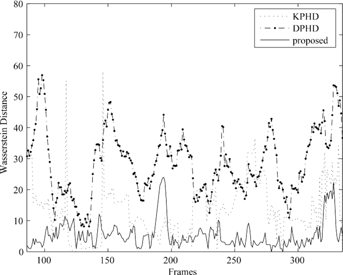
5. Results

The pedestrian sequence from the CAVIAR data set is used as a test video. Figure 1 indicates that PHD filter-based visual trackers can deal with a variable number of targets tracking problems without data association. Figure 1 presents the detection results by a background subtraction detector. Figure 1 shows the particle PHD filter directly using detection results as measurements (denoted as DPHD) would like to generate some false state estimates due to inaccurate detection such as person detection splitting into several blobs. Figure 1 shows the particle PHD filter with observation likelihood based on color histogram and K-means clustering (denoted as KPHD) can avoid failures due to inaccurate detection but output state estimates without satisfying accuracy. Figure 1 demonstrates that more accurate state estimates can be filtered and extracted effectively by our method. Figure 1 shows an example of a slower response of the proposed tracker due to color histogram variation of the candidate target region suffering occlusion. Moreover, it can be derived that the appearance variation of targets due to illumination change and occlusion, as well as regions of background with similar color histograms to targets would mislead the tracker using color histograms only. To improve the tracker additional information is needed.

Fig. 1

Detecting and tracking results of frames 155, 280, and 330 and an example of failure modality in frames 104, 113, and 125: (a) detection results of background subtraction; (b) tracking by DPHD; (c) tracking by KPHD; (d) the proposed method; (e) an example of failures of the proposed method.

The Wasserstein distance⁵ is introduced here to evaluate the performance of trackers. In Fig. 2, the comparison of Wasserstein distance of the three trackers is provided and it demonstrates that our tracker is the best.

Fig. 2

Comparison results of Wasserstein distance for DPHD, KPHD, and the proposed method.

6. Conclusions and Discussion

In this paper, we have presented a robust multitarget visual tracking framework based on the PHD filter which stabilizes the tracker by incorporating color histograms of targets and their temporal dynamics in a unifying framework and improving the accuracy of state extraction using the proposed GMM clustering method. Experiments show the proposed framework can effectively track a varying number of targets with more accurate state estimates. Possible topics of future work include the incorporation of brightness gradient into the appearance model for more robust observation likelihood and the development of a more efficient particle clustering method.

Acknowledgments

This paper is jointly supported by the National Natural Science Foundation of China ( 61074106) and China Aviation Science Foundation ( 2009ZC57003).

References

1.

R. Mahler, “Multitarget filtering using a multitarget first-order moment statistic,” Proc. SPIE, 4380 184 –195 (2001). https://doi.org/10.1117/12.436947 Google Scholar

2.

E. Maggio, M. Taj, and A. Cavallaro, “Efficient multitarget visual tracking using random finite sets,” IEEE Trans. Circuits Syst. Video Technol., 18 (8), 1016 –1027 (2008). https://doi.org/10.1109/TCSVT.2008.928221 Google Scholar

3.

B. N. Vo, S. Singh, and A. Doucet, “Sequential Monte Carlo implementation of the PHD filter for multi-target tracking,” 792 –799 (2003). Google Scholar

4.

D. Comaniciu, V. Ramesh, and P. Meer, “Real-time tracking of non-rigid objects using mean shift,” 142 –149 (2000). Google Scholar

5.

B. N. Vo and W. K. Ma, “The Gaussian mixture probability hypothesis density filter,” IEEE Trans. Signal Process., 54 (11), 4091 –4104 (2006). https://doi.org/10.1109/TSP.2006.881190 Google Scholar

Citation Download Citation

Jingjing Wu, Shiqiang Hu, and Yang Wang "Particle probability hypothesis density filtering for multitarget visual tracking with robust state extraction," Optical Engineering 50(9), 090502 (1 September 2011). https://doi.org/10.1117/1.3638121

Published: 1 September 2011

Access the abstract

JOURNAL ARTICLE
4 PAGES

DOWNLOAD PAPER SAVE TO MY LIBRARY

GET CITATION

RIGHTS & PERMISSIONS

Get copyright permission Get copyright permission on Copyright Marketplace

KEYWORDS

Optical tracking

Particles

Electronic filtering

Expectation maximization algorithms

Detection and tracking algorithms

Particle filters

Visualization

1.

Introduction

Eq. 1

Eq. 2

Eq. 3

2.

Tracking Model

Eq. 4

Eq. 5

Eq. 6

Eq. 7

3.

GMM Clustering

Eq. 8

Eq. 9

4.

Particle PHD Filter-Based Visual Tracker with Robust State Extraction

5.

Results

Fig. 1

Fig. 2

6.

Conclusions and Discussion

Acknowledgments

References

Show All Keywords

Keywords/Phrases

Search In:

Publication Years