Beam wander analysis for focused partially coherent beams propagating in turbulence

Xifeng Xiao; David G. Voelz

doi:10.1117/1.OE.51.2.026001

1 March 2012 Beam wander analysis for focused partially coherent beams propagating in turbulence

Xifeng Xiao, David G. Voelz

Author Affiliations +

Optical Engineering, Vol. 51, Issue 2, 026001 (March 2012). https://doi.org/10.1117/1.OE.51.2.026001

Abstract

We extend the theory of beam wander for propagation through atmospheric turbulence to the case of a focused partially coherent beam (PCB). In addition to investigating the beam wander expression, we restate expressions for the beam size, long- and short-time average beam intensity profile, and the on-axis scintillation index of tracked and untracked beams. A wave optics simulation is implemented and the numerical results are compared with corresponding analytic results. The cases examined involve turbulence strengths ranging from C_n² = 10−16 to 10−14 m−2/3 and for various horizontal paths ranging from 1 to 10 km. Although the extended analytic theory stems from a study of coherent beams, the simulation results show good agreement with the analytical results for PCBs in fluctuation regimes ranging from weak to intermediate.

1. Introduction

Beam wander refers to the gross displacement of an optical beam intensity pattern relative to the pattern for an ideal (vacuum) propagation. Beam wander behavior and related attributes, such as root mean square (RMS) centroid and scintillation index, are important performance indicators of optical beams propagating through turbulence.¹^–³ These beam characteristics have been studied extensively by many researchers over the last five decades through different approaches and for a variety of beam types.⁴^–⁸ The beam wander of a single ray was examined by Beckmann and Chernov using a geometrical optics (GO) approximation.⁴^,⁹ An expression for the wander of a Gaussian beam was first developed using a Huygens–Fresnel approach,⁵ and later was derived by applying a Markovian random process approximation and Ehrenfest’s theorem from quantum mechanics.¹⁰^,¹¹ Eyyuboglu, Cil, and Baykal evaluated the beam wander behavior for several different beam types such as dark-hollow, flat-topped, annular, cos, and cosh-Gaussian beams.¹²^,¹³ Beam wander effects for a spatially PCB were investigated by Berman et al., who introduced a photon distribution function method.¹⁴ To the best of our understanding, the effect of an average phase curvature applied to the PCB, for example “focus,” was not included in the study.

Recently, Andrews and Phillips developed expressions for the beam wander of a focused coherent Gaussian beam in a weak fluctuation turbulence regime by applying Rytov theory.¹⁵ Subsequently, Recolons et al. compared the theoretical models with simulations, and satisfactory agreement was observed.¹⁶ In terms of free space optical (FSO) applications, a convergent PCB or a PCB with some other specified wavefront curvature can greatly improve link performance.¹⁷ However, a convergent beam can still have a significant wander component. This brings us to the question: How does a focused PCB wander when propagating through turbulence?

In this paper, we extend the beam wander theory of Andrews and Phillips to include the focused PCB case. We examine the beam wander (RMS beam centroid) behavior and, in addition, investigate the beam size, the scintillation index, and the mean intensity patterns for both tracked and untracked beams. For validation purposes, a numerical wave optics simulation (WOS) is implemented to create focused PCBs and model their propagation through turbulence. Results are presented and compared with the analytic models for scenarios with turbulence strength varying from weak to strong and propagation distances ranging from 1 to 10 km.

2. Beam Wander Theory

2.1.

Beam Wander Variance

Beam wander can be characterized by the transverse movement $r_{c}$ of the “hot spot” within the beam profile. The general expression of the beam wander variance, $〈 r_{c}^{2} 〉$ , was modeled by Andrews and Phillips as:¹⁵

Eq. (1)

〈 r_{c}^{2} 〉 = 4 π^{2} k^{2} W^{2} (Z) \int_{0}^{Z} \int_{0}^{\infty} κ Φ_{n} (κ) H_{LS} (κ, z) [1 - e^{- Λ_{P} Z κ^{2} {(1 - z / Z)}^{2} / k}] d κ d z,

where

κ

is the spatial wave number,

k

is the optical wave number defined by

k = 2 π / λ

and

λ

is the wavelength.

Z

is the propagation distance from the transmitter to the receiver, and

z

is a distance variable that ranges from 0 to

Z

. The parameter

Λ_{P}

is defined and discussed below.

H_{LS} (κ, z)

is a filter function that selects the low spatial frequencies in the turbulence power spectrum

Φ_{n} (κ)

that correspond to large spatial scales. In our work the filter function was applied in the same manner for all turbulence regimes, weak through strong. The filter function can be expressed as

Eq. (2)

H_{LS} (κ, z) = \exp [- κ^{2} W^{2} (z)],

where

W (z)

is the free space beam radius (or beam size) at distance

z

. For a focused PCB with an initial beam size

W_{0}

, a phase-front curvature

F

and coherence length

l_{c}

, we have¹⁸^,¹⁹

Eq. (3)

W (z) = W_{0} {[{(1 - \frac{z}{F})}^{2} + (1 + \frac{2 W_{0}^{2}}{l_{c}^{2}}) {(\frac{2 z}{k W_{0}^{2}})}^{2}]}^{1 / 2} .

The coherence length

l_{c}

is a measure of the transverse spatial correlation of the beam source field. When

l_{c}

is on the order of

W_{0}

, the effect on the beam size can be significant.

l_{c}

is infinite for a perfectly coherent beam.

Returning to Eq. (1), we now define the nondimensional output beam parameter $Λ_{\overset{}{P}}$ of a PCB, and it can be written as

Eq. (4)

Λ_{P} = \frac{2 Z}{k W^{2} (Z)} .

Typically,

Φ_{n} (κ)

in Eq. (1) is assumed to be the Kolmogorov spectrum, which is defined as

Eq. (5)

Φ_{n} (κ) = 0.033 C_{n}^{2} κ^{- 11 / 3},

where

C_{n}^{2}

is the refractive index structure parameter and is assumed to be constant for horizontal propagation. Apply the geometrical optics (GO) approximation and the last term in Eq. (1) becomes:

Eq. (6)

1 - e^{- Λ_{P} Z κ^{2} {(1 - z / Z)}^{2} / k} \approx \frac{Λ_{P} Z κ^{2} {(1 - z / Z)}^{2}}{k}, if \frac{Λ_{P} Z κ^{2}}{k} ≪ 1 .

Inserting Eq. (6) into Eq. (1) and calculating the integrations, we obtain the beam wander variance:¹⁵

Eq. (7)

〈 r_{c}^{2} 〉 = 7.25 C_{n}^{2} Z^{3} W_{0}^{- 1 / 3} \int_{0}^{\overset{}{Z}} {(1 - \frac{z}{Z})}^{2} G_{P} {(z)}^{- 1 / 6} d z,

where

G_{\overset{}{P}} (z)

is a function defined for the focused PCB beam as

Eq. (8)

G_{P} (z) = {[W (z) / W_{0}]}^{2} .

For coherent beams, the second term in the bracket of the definition for

W (z)

[Eq. (3)] is typically negligible and is often dropped to simplify the calculation of

G_{P} (z)

¹⁵. For PCBs, this term could be significant and cannot be ignored. A closed-form analytic solution of Eq. (7) with Eq. (8) included is attainable and involves a hypergeometric function that is typically evaluated numerically. For the results in this paper, we bypass this step and simply evaluate Eq. (7) directly using numerical integration.

2.2.

Mean Intensity Profiles

Consider a beam with the field $U (r, z)$ , where $r$ is the transverse distance from the beam center in the plane perpendicular to the propagation direction. For a unit-amplitude field at the source plane ( $z = 0$ ), we have:

Eq. (9)

U (r, 0) = \exp (- \frac{r^{2}}{W_{0}^{2}} - i \frac{k r^{2}}{2 F}) \exp [i ξ (r, 0)],

where

ξ (r, 0)

is the random phase function to characterize the partially coherent beam at the beam source (

z = 0

) with parameter

l_{c}

. As the beam propagates through turbulence, assuming the average intensity profile at the receiver is Gaussian,²⁰^,²¹ the only free parameter that governs the beam profile is the receiving beam size/radius. Following Fante, who considered long-time (LT) and short-time (ST) averages, which correspond to untracked and tracked beams, respectively, the respective beam size values,

W_{LT} (Z)

and

W_{ST} (z)

, are related by:⁶

Eq. (10)

{W_{ST}}^{2} (Z) = {W_{LT}}^{2} (Z) - 〈 r_{c}^{2} 〉,

where

〈 r_{c}^{2} 〉

is the beam wander variance. Expressions for

W_{LT} (Z)

have been developed in several recent publications. We compared expressions presented by Andrews and Phillips, Ricklin and Davidson, and Korotkova et al. for the LT average beam size and irradiance distribution, and found that for a coherent Gaussian beam propagated over a relatively short distance and/or through weak turbulence, the theories from these authors¹⁵^,²²^,²³ are almost identical and are consistent with our wave optics simulation results. However, for propagation through stronger turbulence, the theory put forward by Ricklin and Davidson provides a better fit to our simulation results. This expression for the LT average beam size is given by:²²

Eq. (11)

W_{LT} (Z) = W_{0} {[{(1 - \frac{Z}{F})}^{2} + (1 + \frac{2 W_{0}^{2}}{l_{c}^{2}} + \frac{2 W_{0}^{2}}{ρ_{0}^{2}}) {(\frac{2 Z}{k {\overset{}{W}}_{0}^{2}})}^{2}]}^{1 / 2},

where

ρ_{0}

is defined as the coherence length of a spherical wave propagating in turbulence and is given by

Eq. (12)

ρ_{0} = {(0.55 C_{n}^{2} k^{2} Z)}^{- 3 / 5} .

Consequently, the mean intensity profiles of the LT and ST beams at the receiver,

I_{LT} (r, Z)

, and

I_{ST} (r, z)

, can be written as:¹⁵^,²²

Eq. (13)

I_{LT} (r, Z) = \frac{W_{0}^{2}}{{W_{LT}}^{2} (Z)} \exp [- \frac{2 r^{2}}{{W_{LT}}^{2} (Z)}],

and

Eq. (14)

I_{ST} (r, Z) = \frac{W_{0}^{2}}{{W_{ST}}^{2} (Z)} \exp [- \frac{2 r^{2}}{{W_{ST}}^{2} (Z)}] .

2.3.

Scintillation Theory (On-Axis)

To be consistent with previous work on scintillation, we use the terms “tracked” for ST average results and “untracked” for LT average results in this section. The derivations of the on-axis scintillation indices of tracked and untracked coherent beams have been thoroughly discussed in several papers listed in Refs. 8 and 15. Corresponding analytical expressions for a focused PCB beam are found by incorporating the PCB beam size formulation. For a tracked beam, the on-axis scintillation index in weak turbulence is given by

Eq. (15)

σ_{I, tr, weak}^{2} (Z) = 3.86 σ_{R}^{2} {0.4 {[{(1 + 2 Θ_{P})}^{2} + 4 Λ_{P}^{2}]}^{5 / 12} \cos [\frac{5}{6} \tan^{- 1} (\frac{1 + 2 Θ_{P}}{2 Λ_{P}})] - \frac{11}{16} Λ_{P}^{5 / 6}},

where

Θ_{\overset{}{P}}

is a nondimensional PCB output beam parameter given by

Eq. (16)

Θ_{\overset{}{P}} = \frac{1 - \frac{Z}{F}}{{(1 - \frac{Z}{F})}^{2} + {(\frac{2 Z}{k W_{0}^{2}})}^{2} (1 + \frac{2 W_{0}^{2}}{l_{c}^{2}})},

and

{σ_{R}}^{2}

is the Rytov variance given by

Eq. (17)

σ_{R}^{2} = 1.23 C_{n}^{2} k^{7 / 6} Z^{11 / 6} .

For an untracked beam, the on-axis scintillation index is

Eq. (18)

σ_{I, un, weak}^{2} (Z) = 4.42 σ_{R}^{2} Λ_{P}^{5 / 6} \frac{σ_{pe}^{2}}{W^{2} (Z)} + σ_{I, tr}^{2} (Z),

where

{σ_{pe}}^{2}

is the jitter-induced pointing error variance. For a focused PCB beam

Eq. (19)

{σ_{pe}}^{2} = 7.25 C_{n}^{2} Z^{3} W_{0}^{- 1 / 3} \int_{0}^{\overset{}{Z}} {(1 - \frac{z}{Z})}^{2} {{[\frac{1}{G_{P} (z)}]}^{1 / 6} - {[\frac{K_{r}^{2} W_{0}^{2}}{1 + K_{r}^{2} W_{0}^{2} G_{P} (z)}]}^{1 / 6}} d z,

where

Eq. (20)

K_{r} = \frac{2 π}{2.1 ρ_{0}} .

Equations (15) and (18) are restricted to weak turbulence. Under intermediate to strong turbulence, we follow the theory developed by Andrews and Phillips,¹⁵ which yields the general expression for the scintillation index for a tracked beam

Eq. (21)

σ_{I, tr}^{2} (Z) = \exp {\frac{0.49 σ_{I, tr, weak}^{2} (Z)}{{[1 + 0.56 (1 + Θ_{P}) σ_{I, tr, weak}^{12 / 5} (Z)]}^{7 / 6}} + \frac{0.51 σ_{I, tr, weak}^{2} (Z)}{{[1 + 0.69 σ_{I, tr, weak}^{12 / 5} (Z)]}^{5 / 6}}} - 1,

and for an untracked beam

Eq. (22)

σ_{I, un}^{2} (Z) = 4.42 σ_{R}^{2} {(\frac{2 Z}{k})}^{5 / 6} \frac{σ_{Pe}^{2}}{W_{LT}^{11 / 3} (Z)} + σ_{I, tr}^{2} (Z) .

3. Wave Optics Simulations

Comparison of analytic values with numerical WOS results helps validate both the theory and simulation modeling approaches. In addition, the numerical approach can help verify that the GO approximation used in the analytic result is acceptable. The WOS approach has been discussed in detail in various publications.²⁴^–²⁶ For a focused PCB simulation we follow the approach developed for a collimated PCB but with a phase curvature term applied at the source plane.²⁷^–²⁹ Specifically, the implementation procedure can be described as follows: (1) generate a random phase screen with appropriate spatial coherence length $l_{c}$ ;²⁹ (2) apply the phase screen to a coherent beam in the source plane; (3) numerically “propagate” the beam to the observation plane²⁸ through a separate set of phase screens that model atmospheric turbulence and compute the intensity; and (4) repeat steps 1 to 3 $N_{PS}$ times, each time with a different realization of the spatial coherence screen (but without changing the turbulence screen realizations) and average the intensity at the observation plane. The average intensity is the PCB result. We typically limit $N_{PS}$ to 30 to reduce computation time.

Atmospheric turbulence is simulated with a split-step approach involving a series of random screens evenly spaced along the propagation path.³⁰ Our turbulence screens assume a Kolmogorov spectrum. The number of turbulence screens ( $N_{TS}$ ) used for a particular scenario is determined following the criteria described in Ref. 24. For each data point presented, 500 propagations are simulated through different realizations of turbulence, which means a total of $N_{PS} \times N_{TS} = 30 \times 500 = 15, 000$ propagations are required for each point. Both LT (untracked) and ST (tracked) cases are investigated. For ST (tracked) results, the beam centroid for each of the 500 turbulence realizations is found and each intensity pattern is translated to the center of the numerical grid before the measures are computed. The WOS program codes were implemented in the MATLAB environment.

The link parameters for results presented in this paper are listed in Table 1. The analysis and simulations can be applied to wide range of parameters, but the choices here are characteristic of moderate-length terrestrial links (1 to 10 km) in weak ( $σ_{R}^{2} < 1$ ) to strong ( $σ_{R}^{2} > 1$ ) intensity fluctuation regimes. The phase curvature parameter $F$ is set equal to the propagation distance $Z$ so the effect of focus over a range of distances can be investigated. PCB coherence lengths of 2 and 5 cm are typical of values that provide near-optimal link performance in applications like FSO communications.¹⁷

Table 1

WOS simulation parameters for link scenarios studied in this paper.

Scenario parameters	$C_{n}^{2}$	$σ_{R}^{2}$	$N_{TS}$
$W_{0} = 5 cm$ , $λ = 1 μm$ , $Z = 1$ to 10 km, $F = Z$ , $l_{c} = 2$ or 5 cm	$10^{- 16} m^{- 2 / 3}$	0.003 to 0.23	2
	$10^{- 15} m^{- 2 / 3}$	0.03 to 2.3	2 to 6
	$10^{- 14} m^{- 2 / 3}$	0.3 to 22.7	2 to 20

Limiting the number of PCB phase screens ( $N_{PS} = 30$ ) when performing the turbulence simulations saves computation time but introduces additional fluctuations in the results, especially when $l_{c}$ is relatively small. To compensate for this effect, we simulate propagation through vacuum and calculate the beam wander variance ${〈 r_{c}^{2} 〉}_{V}$ and scintillation index $σ_{c, V}^{2}$ that are purely caused by the limited number of PCB screens. To illustrate the magnitude of these errors, Fig. 1 presents vacuum results for $l_{c} = 2$ and 5 cm. The false beam wander variance increases roughly in a linear fashion with propagation distance but the false scintillation index for both tracked and untracked beams tends to be independent of $Z$ . The values are larger for the shorter coherence length. In the next section we define how corrections are implemented to compensate for the effects of using a limited number of PCB screens.

Fig. 1

False beam wander variance ${〈 {r_{c}}^{2} 〉}_{V}$ (a) and (c) and false on-axis intensity variance $σ_{I, V}^{2}$ (b) and (d) induced by the PCB WOS approach. The coherence length is $l_{c} = 2 cm$ (a) and (b) and 5 cm (c) and (d). Tracked (▪) and untracked (★) beam results are shown. Other link parameters are listed in Table 1.

4. Analytic and WOS Results

In this section we present examples of analytic and WOS beam size, beam wander, and scintillation index results. However, a few example irradiance profiles are first presented to illustrate the characteristics of an average PCB propagated through turbulence. Figure 2 shows analytic tracked (ST) and untracked (LT) profiles created with Eqs. (13) and (14) and corresponding WOS results. In general, the profiles are Gaussian in shape and the tracked beams have higher peak intensities than the untracked beams. These examples also illustrate the close match between the analytic and WOS results. We reiterate that all the results in this section assume the beam is being focused for the indicated propagation distance.

Fig. 2

Tracked (▪ and ---) and untracked (★ and —) beam intensity profiles for $C_{n}^{2} = 10^{- 15} m^{- 2 / 3}$ and (a) $l_{c} = 5 cm$ , $Z = 2.5 km$ ; (b) $l_{c} = 2 cm$ , $Z = 9 km$ . Markers denote WOS results and lines denote analytical results. $F = Z$ and other link parameters are as listed in Table 1.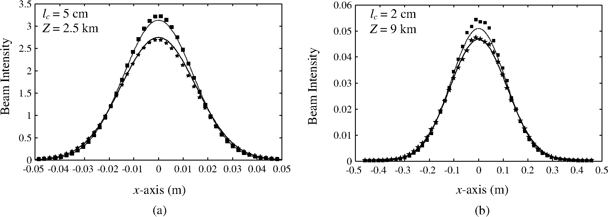

4.1.

Beam Size

The analytic expressions for LT and ST average beam sizes are given in Eqs. (10) and (11). For the WOS results, the first step in finding the LT beam size is averaging the two-dimensional intensity profiles produced by the 500 turbulence realizations and measuring the $e^{- 2}$ irradiance radius. This gives an initial estimate of the beam size $W_{LT, S, 0}$ . The beam size corrected for effects of a limited number of PCB screens is given by

Eq. (23)

W_{LT, S} = \sqrt{W_{LT, S, 0}^{2} - {〈 r_{c}^{2} 〉}_{\overset{}{V}}} .

The false beam wander value

{〈 r_{c}^{2} 〉}_{V}

in Eq. (23) is the RMS beam centroid variance calculated from a set of vacuum propagations performed with the identical PCB screens used in the turbulence propagations. On the other hand, the ST beam size,

W_{ST, S}

is found by first translating each beam in the turbulence propagation set so the centroid is in the center of the numerical grid. The beam irradiance patterns are averaged and the

e^{- 2}

irradiance radius is found. Any additional centroid motion due to the limited number of PCB screens is also removed in the processing, so no correction is applied to the

W_{ST, S}

values.

Analytic and WOS beam size results are presented in Fig. 3. As expected, the beam size increases with propagation/focus distance, stronger turbulence, and smaller coherence length. The analytic and WOS results are consistent in all cases for the turbulence strengths of $C_{n}^{2} = 10^{- 16}$ and $10^{- 15} m^{- 2 / 3}$ . For the stronger turbulence case of $C_{n}^{2} = 10^{- 14} m^{- 2 / 3}$ and with the tracked beam, the analytic prediction has somewhat higher values than the WOS results.

Fig. 3

Tracked (left) and untracked (right) beam size results as a function of $Z$ for $l_{c} = 2 cm$ (top) and 5 cm (bottom). Analytic results are solid lines and WOS results are indicated with markers. Turbulence strength: $C_{n}^{2} = 10^{- 14} m^{- 2 / 3}$ (★), $10^{- 15} m^{- 2 / 3}$ (▪), and $10^{- 16} m^{- 2 / 3}$ (•). $F = Z$ and other link parameters are given in Table 1.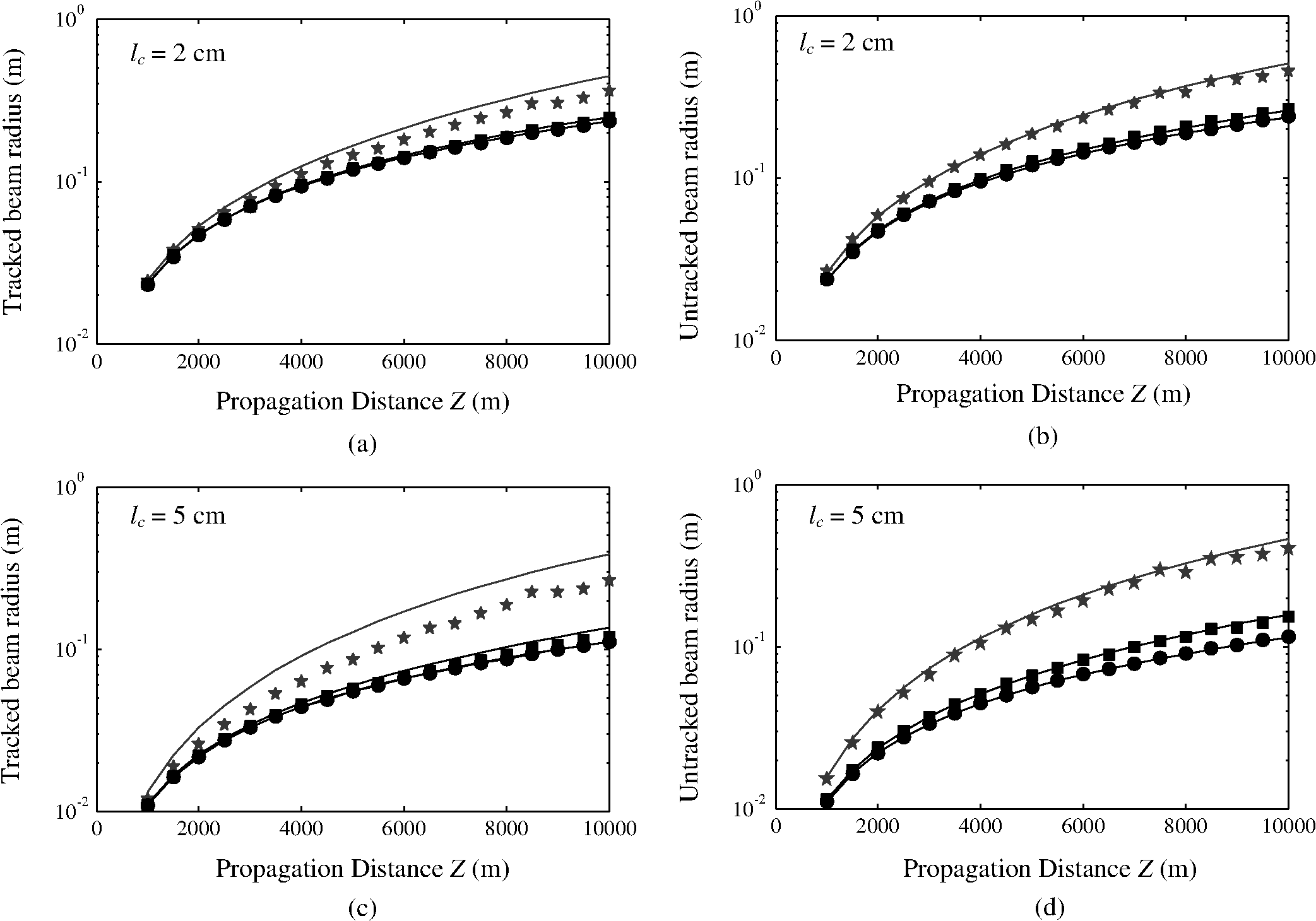

4.2.

Beam Wander

The analytic beam wander result is given in Eq. (7). The corrected WOS result ${〈 r_{c}^{2} 〉}_{S}$ is obtained via

Eq. (24)

{〈 r_{c}^{2} 〉}_{S} = W_{LT, S}^{2} - W_{ST, S}^{2} .

Figure 4 shows comparisons of the analytical and WOS results. The wander increases with propagation/focus distance and also with turbulence strength. Dependence on the coherence length

l_{c}

is weak for the cases presented. The analytic and WOS results are generally consistent, although the WOS tends to produce slightly larger beam wander values. This trend is most obvious in the strong turbulence case (

C_{n}^{2} = 10^{- 14} m^{- 2 / 3}

) at longer propagation/focus distances.

Fig. 4

RMS centroid position (beam wander) as a function of $Z$ for $l_{c} = 2 cm$ (a) and 5 cm (b). Analytic results are solid lines and WOS results are indicated with markers. Turbulence strength: $C_{n}^{2} = 10^{- 14} m^{- 2 / 3}$ (★), $C_{n}^{2} = 10^{- 15} m^{- 2 / 3}$ (▪), and $C_{n}^{2} = 10^{- 16} m^{- 2 / 3}$ (•). $F = Z$ and other link parameters are given in Table 1.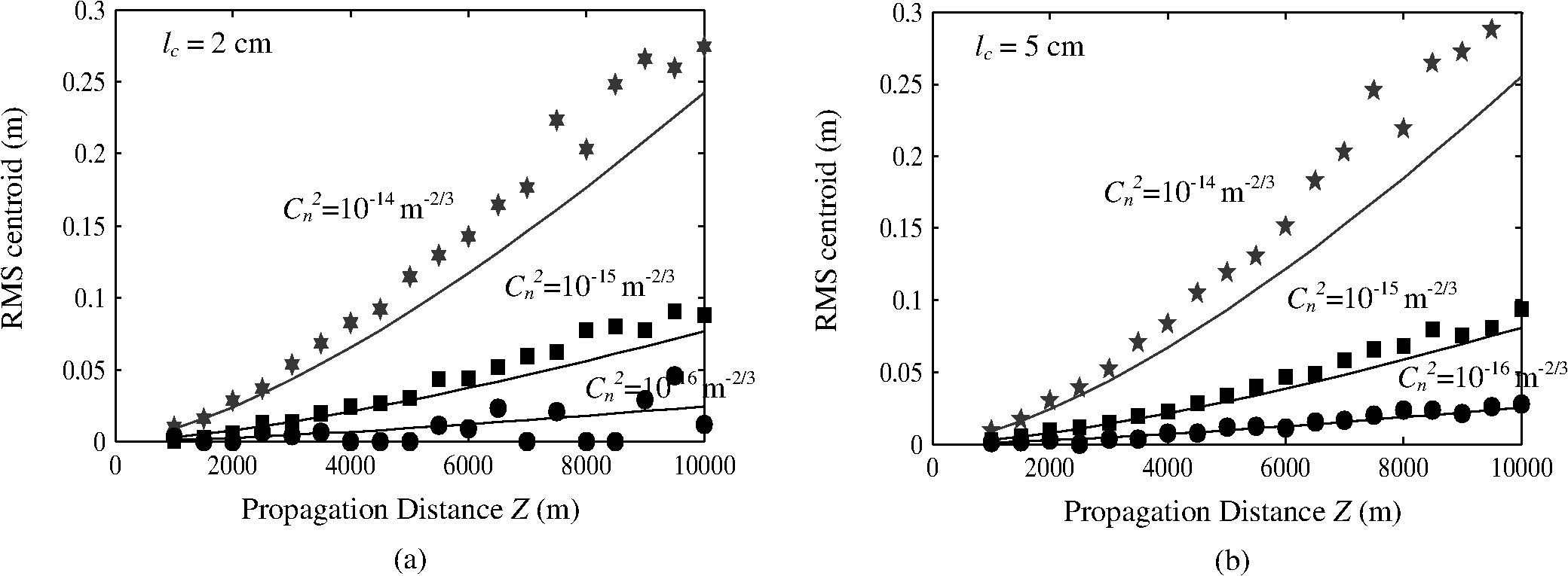

4.3.

Scintillation Index

The analytic scintillation index expressions (on-axis) for tracked and untracked beams are given in Eqs. (21) and (22). For the WOS, the scintillation index is found by computing the normalized variance of the irradiance at the center of numerical grid (optical axis) for the 500 turbulence realizations. Again, the tracked results include the translation of the beam to remove the centroid wander. To compensate for the effects of the finite number of PCB phase screens, the following is used:²³

Eq. (25)

σ_{I, S}^{2} = \frac{σ_{I, S, 0}^{2} - σ_{I, V}^{2}}{1 + σ_{I, V}^{2,}},

where

σ_{I, S, 0}^{2}

is the initial scintillation index computed from the WOS results,

σ_{I, V}^{2}

is the false index computed for vacuum propagations with only the PCB phase screens applied, and

σ_{I, S}^{2}

is the corrected scintillation index.

Figure 5 presents the scintillation results. In general, the index values increase with distance and turbulence strength. The WOS values generally follow the analytic results, although there is clearly more scatter in the WOS points for the $l_{c} = 2 cm$ cases. This is likely due to imperfect correction for the limited number of PCB screens. Saturation of the index value is evident at longer distances for the stronger turbulence cases. We note that for increasing distance beyond that shown in Fig. 5, and therefore increasing Rytov variances, the focused PCB index values appear to peak and then reduce to a saturation value in a way that is similar to results for coherent beams.³¹ We expect the saturation regime for a PCB to occur at larger Rytov variances than for a comparable coherent beam.¹⁸ However, further study of this regime would likely require: (1) inclusion of a finite inner scale in the turbulence spectrum, as the scintillation index is highly sensitive to the inner scale; and (2) the exploration of WOS approaches that accurately model the strong fluctuation regime, likely involving high densities of grid points and turbulent screens.

Fig. 5

On-axis scintillation index as a function of $Z$ for tracked (left) and untracked (right) beams and $l_{c} = 2 cm$ (top) and 5 cm (bottom). Analytic results are solid lines and WOS results are indicated with markers. Turbulence strength: $C_{n}^{2} = 10^{- 14} m^{- 2 / 3}$ (★), $C_{n}^{2} = 10^{- 15} m^{- 2 / 3}$ (▪), and $C_{n}^{2} = 10^{- 16} m^{- 2 / 3}$ (•). $F = Z$ and other link parameters are given in Table 1.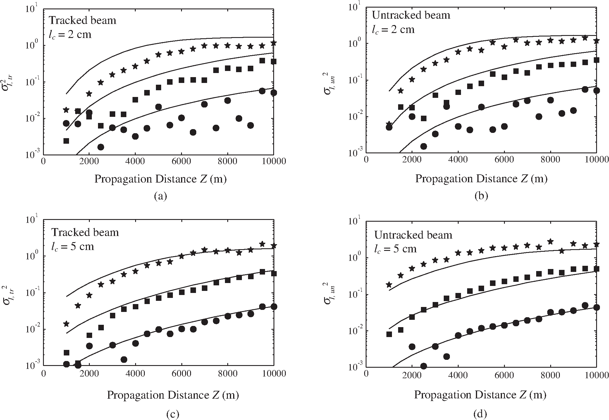

5. Conclusion

The extension of coherent beam wander theory to the case of a focused PCB essentially involves the substitution of the beam waist expression that includes the PCB parameters. Comparison of the resulting analytic expressions for beam size, beam wander, and on axis-scintillation index with WOS results indicates that the GO approximation used in the coherent theory appears reasonable for the PCB theory, at least for most of the link values we studied. The WOS results required corrections for errors caused by the use of a limited number of PCB phase screens. Differences between the analytic and WOS results were primarily seen in stronger turbulence situations. The differences could be due to the use of the Rytov approximation in the analytic derivations but also to numerical issues in the WOS—for example, incomplete correction of the error due to the limited number of PCB screens.

Acknowledgments

This work was supported by the Air Force Office of Scientific Research under the Sensing, Surveillance, and Navigation program, grant FA9550-09-1-0616.

References

1.

F. Dioset al., “Scintillation and beam-wander analysis in an optical ground station-satellite uplink,” Appl. Opt., 43 (19), 3866 –3873 (2004). http://dx.doi.org/10.1364/AO.43.003866 APOPAI 0003-6935 Google Scholar

2.

L. C. Andrewset al., “Strehl ratio and scintillation theory for uplink Gaussian-beam waves: Beam wander effects,” Opt. Eng., 45 (7), 076001 (2006). http://dx.doi.org/10.1117/1.2219470 OPENEI 0892-354X Google Scholar

3.

D. H. Tofsted, “Outer-scale effects in beam-wander and angle-of-arrival variances,” Appl. Opt., 31 (27), 5865 –5870 (1992). http://dx.doi.org/10.1364/AO.31.005865 APOPAI 0003-6935 Google Scholar

4.

P. Beckmann, “Signal degeneration in laser beams propagated through a turbulent atmosphere,” Radio Sci., 69D (4), 629 –640 (1965). RASCAD 0048-6604 Google Scholar

5.

G. A. AndreevE. I. Gelfer, “Angular random walks of the center of gravity of the cross section of a diverging light beam,” Radiophys. Quantum Electron., 14 (9), 1145 –1147 (1971). RPQEAC 0033-8443 Google Scholar

6.

R. L. Fante, “Electromagnetic beam propagation in turbulent media,” Proc. IEEE, 63 (12), 790 –811 (1975). http://dx.doi.org/10.1109/PROC.1975.10035 IEEPAD 0018-9219 Google Scholar

7.

J. H. ChurnsideR. L. Lataitis, “Wander of an optical beam in the turbulent atmosphere,” Appl. Opt., 29 (7), 926 –930 (1990). http://dx.doi.org/10.1364/AO.29.000926 APOPAI 0003-6935 Google Scholar

8.

G. J. BakerR. S. Benson, “Gaussian-beam weak scintillation on ground-to-space paths: compact descriptions and Rytov-method applicability,” Opt. Eng., 44 (10), 106002 (2005). http://dx.doi.org/10.1117/1.2076927 OPENEI 0892-354X Google Scholar

9.

L. A. Chernov, Wave Propagation in a Random Medium, Dover, New York (1967). Google Scholar

10.

V. L. MironovV. V. Nosov, “On the theory of spatially limited light beam displacements in a randomly inhomogeneous medium,” J. Opt. Soc. Am., 67 (8), 1073 –1080 (1977). http://dx.doi.org/10.1364/JOSA.67.001073 JOSAAH 0030-3941 Google Scholar

11.

R. J. Cook, “Beam wander in a turbulent medium: an application of Ehrenfest’s theorem,” J. Opt. Soc. Am., 65 (8), 942 –948 (1975). JOSAAH 0030-3941 Google Scholar

12.

H. T. EyyubogluC. Z. Cil, “Beam wander of dark hollow, flat-topped and annular beams,” Appl. Phys. B, 93 (2–3), 595 –604 (2008). APBOEM 0946-2171 Google Scholar

13.

C. Z. Cilet al., “Beam wander characteristics of cos and cosh-Gaussian beams,” Appl. Phys. B, 95 (4), 763 –771 (2009). http://dx.doi.org/10.1007/s00340-009-3553-5 APBOEM 0946-2171 Google Scholar

14.

G. P. BermanA. A. ChumakV. N. Gorshkov, “Beam wandering in the atmosphere: the effect of partial coherence,” Phys. Rev. E, 76 (5), 056606 (2007). http://dx.doi.org/10.1103/PhysRevE.76.056606 PLEEE8 1063-651X Google Scholar

15.

L. C. AndrewsR. L. Phillips, Laser Beam Propagation through Random Media, SPIE Press, Bellingham, WA (2005). Google Scholar

16.

J. RecolonsL. C. AndrewsR. L. Phillips, “Analysis of beam wander effects for a horizontal-path propagating Gaussian-beam wave: focused beam case,” Opt. Eng., 46 (8), 086002 (2007). http://dx.doi.org/10.1117/1.2772263 Google Scholar

17.

D. K. BorahD. G. Voelz, “Spatially partially coherent beam parameter optimization for free space optical communications,” Opt. Exp., 18 (20), 20746 –20758 (2010). http://dx.doi.org/10.1364/OE.18.020746 OPEXFF 1094-4087 Google Scholar

18.

O. KorotkovaL. C. AndrewsR. L. Phillips, “Model for a partially coherent Gaussian beam in atmospheric turbulence with application in LaserCom,” Opt. Eng., 43 (2), 330 –341 (2004). http://dx.doi.org/10.1117/1.1636185 OPENEI 0892-354X Google Scholar

19.

L. MandelE. Wolf, “Radiation from sources of any state of coherence,” Optical Coherence and Quantum Optics, 229 –337 Cambridge University, pp. 1995). Google Scholar

20.

J. RecolonsL. C. AndrewsR. L. Phillips, “Analysis of beam wander effects for a horizontal-path propagating Gaussian-beam wave: focused beam case,” Opt. Eng., 46 (8), 086002 (2007). http://dx.doi.org/10.1117/1.2772263 OPENEI 0892-354X Google Scholar

21.

H. T. EyyuboğluY. BaykalE. Sermutlu, “Convergence of general beams into Gaussian intensity profiles after propagation in turbulent atmosphere,” Opt. Commun., 265 (2), 399 –405 (2006). http://dx.doi.org/10.1016/j.optcom.2006.03.071 OPCOB8 0030-4018 Google Scholar

22.

J. C. RicklinF. M. Davidson, “Atmospheric turbulence effects on a partially coherent Gaussian beam: implication for free-space laser communication,” J. Opt. Soc. Am. A, 19 (9), 1794 –1802 (2002). http://dx.doi.org/10.1364/JOSAA.19.001794 JOAOD6 0740-3232 Google Scholar

23.

O. KorotkovaL. C. AndrewsR. L. Phillips, “The effect of partially coherent quasi-monochromatic Gaussian beam on the probability of fade,” Proc. SPIE, 5160 68 (2004). http://dx.doi.org/10.1117/12.504174 PSISDG 0277-786X Google Scholar

24.

R. Rao, “Statistics of the fractal structure and phase singularity of a plane light wave propagation in atmospheric turbulence,” Appl. Opt., 47 (2), 269 –276 (2008). http://dx.doi.org/10.1364/AO.47.000269 APOPAI 0003-6935 Google Scholar

25.

S. M. FlatteJ. S. Gerber, “Irradiance-variance behavior by numerical simulation for plane-wave and spherical-wave optical propagation through strong turbulence,” J. Opt. Soc. Am. A, 17 (6), 1092 –1097 (2000). http://dx.doi.org/10.1364/JOSAA.17.001092 JOAOD6 0740-3232 Google Scholar

26.

M. C. RoggemannB. Welsh, Imaging Through Turbulence, 57 –122 CRC Press, Boca Raton, FL (1996). Google Scholar

27.

X. XiaoD. Voelz, “On-axis probability density function and fade behavior of partially coherent beams propagating through turbulence,” App. Opt., 48 (2), 167 –175 (2009). http://dx.doi.org/10.1364/AO.48.000167 APOPAI 0003-6935 Google Scholar

28.

D. Voelz, “Partial coherence simulation,” Computational Fourier Optics, 169 –189 SPIE Press, Bellingham, WA (2011). http://dx.doi.org/10.1117/3.858456.ch9 Google Scholar

29.

X. XiaoD. Voelz, “Wave optics simulation approach for partial spatially coherent beams,” Opt. Exp., 14 (16), 6986 –6992 (2006). http://dx.doi.org/10.1364/OE.14.006986 OPEXFF 1094-4087 Google Scholar

30.

J. Schmidt, Numerical Simulation of Optical Wave Propagation With Examples in MATLAB, 149 –184 SPIE Press, Bellingham, WA (2010). http://dx.doi.org/10.1117/3.866274 Google Scholar

31.

H. T. Eyyuboglu, “Annular, cosh and cos Gaussian beams in strong turbulence,” Appl. Phys. B, 103 (3), 763 –769 (2011). APBOEM 0946-2171 Google Scholar

Biography

Xifeng Xiao received her BS and MS degrees in physics from Xiamen University, Fujian, China, in 1998 and 2001, respectively. She earned her MS and PhD degrees in electrical engineering in 2004 and 2008, respectively, from New Mexico State University, where she is currently a research assistant professor. Her main research includes simulation and modeling of free-space laser communication, liquid-crystal polarization, acousto-optic imaging spectrometer design, and polarimetric imaging.

David G. Voelz is a professor of electrical engineering at New Mexico State University. He received his BS in electrical engineering from New Mexico State University in 1981 and his MS and PhD degrees in electrical engineering from the University of Illinois in 1983 and 1987, respectively. From 1986 to 2001, he was with the Air Force Research Laboratory in Albuquerque, NM. His current research interests include spectral and polarimetric imaging, laser imaging and beam projection, laser communications, adaptive optics, and astronomical instrumentation development.

Citation Download Citation

Xifeng Xiao and David G. Voelz "Beam wander analysis for focused partially coherent beams propagating in turbulence," Optical Engineering 51(2), 026001 (1 March 2012). https://doi.org/10.1117/1.OE.51.2.026001

Published: 1 March 2012

Access the abstract

JOURNAL ARTICLE
9 PAGES

DOWNLOAD PAPER SAVE TO MY LIBRARY

GET CITATION

CITATIONS

Cited by 22 scholarly publications.

Explore citations on Lens.org

RIGHTS & PERMISSIONS

Get copyright permission Get copyright permission on Copyright Marketplace

KEYWORDS

Turbulence

Beam propagation method

Scintillation

Beam analyzers

Atmospheric propagation

Optical simulations

Wave propagation

1.

Introduction

2.

Beam Wander Theory

2.1.

Beam Wander Variance

Eq. (1)

Eq. (2)

Eq. (3)

Eq. (4)

Eq. (5)

Eq. (6)

Eq. (7)

Eq. (8)

2.2.

Mean Intensity Profiles

Eq. (9)

Eq. (10)

Eq. (11)

Eq. (12)

Eq. (13)

Eq. (14)

2.3.

Scintillation Theory (On-Axis)

Eq. (15)

Eq. (16)

Eq. (17)

Eq. (18)

Eq. (19)

Eq. (20)

Eq. (21)

Eq. (22)

3.

Wave Optics Simulations

Table 1

Fig. 1

4.

Analytic and WOS Results

Fig. 2

4.1.

Beam Size

Eq. (23)

Fig. 3

4.2.

Beam Wander

Eq. (24)

Fig. 4

4.3.

Scintillation Index

Eq. (25)

Fig. 5

5.

Conclusion

Acknowledgments

References

Biography

Show All Keywords

Keywords/Phrases

Search In:

Publication Years