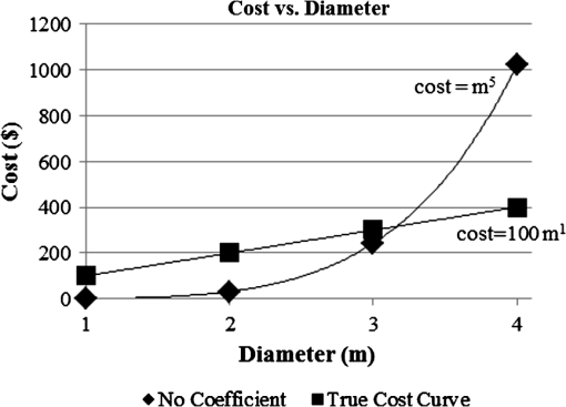
1.

Introduction

In 2005, Stahl et al. published a multivariable cost model for ground telescopes.¹ Stahl focused on the cost of the optical telescope assembly (OTA), where OTA is defined to include the primary mirror, secondary mirror, and the related support structure. The model presented includes primary mirror diameter, diffraction-limited wavelength, and year of development as major cost drivers. As published in the paper, the model is:

Stahl observes that all of the signs in the multivariate model are in agreement with engineering judgment. Specifically, cost increases with diameter, decreases with diffraction-limited wavelength, and decreases with year. Overall the model has good statistical fit ($R^2=95\%$, adjusted $R^2=94\%$, $\mathrm{SPE}=35\%$). The exponents for segment diameter, diffraction-limited wavelength, and year of development were all derived using maximum likelihood estimation on a sample size of 14 telescopes. For more information on the data used to develop the model, see Ref. 2.

In preparation for an upcoming multivariable cost model for space telescopes, the 2005 ground data was revisited as a training set to test new methods. While the multivariable model published in Stahl et al. was verified, an inconsistency in the single-variable model coefficient was observed. Specifically, the single-variable model excluded a leading multiplier, thereby inflating the estimate for the diameter exponent. Additionally, new methods were considered to account for different prescriptions in the multivariable learning curve model.

2.

Leading Multipliers

Although all single-variable cost models should have a leading multiplier, cost models frequently exclude leading multipliers because most design decisions are based on relative price differences rather than absolute price estimates. Thus engineers are generally more interested in the rate at which cost varies with an explanatory variable (e.g., diameter) than in the actual cost estimate of a telescope for a given set of telescope parameters. Nonetheless, the presence of the leading multiplier is crucial to finding the correct relative relationship between cost and telescope parameters. To formalize the above discussion, consider fitting a model of the form $\text{Cost}={KD}^{\alpha }$ for leading multiplier $K$, diameter $D$, and exponent $\alpha$. A model that excludes the leading multiplier is of the form $\text{Cost}=D^{\alpha }$. Here, we start with a trivial example and then present the change to the ground telescope cost model.

Before the example, we note that changing the units for diameter should not affect the exponent $\alpha$. To understand why this is the case, it is instructive to interpret $\alpha$. For $\alpha$ less than 2, it is less expensive to build a large aperture telescope than a smaller aperture telescope in terms of collecting area since area scales with the square of diameter. For $\alpha$ greater than 2, it is less expensive to build a small aperture telescope in terms of collecting area, and for $\alpha$ equal to 2, cost per photon is independent of diameter. Thus, $\alpha$ has a straightforward interpretation that should be independent of the chosen units for diameter.

Omitting the leading multiplier immediately violates the independence of $\alpha$ to units. Suppose a power model is to be constructed for the cost data in Table 1. Clearly cost scales linearly with diameter in centimeters, with a leading multiplier of 1. For diameter in meters, cost scales linearly with a leading multiplier of 100. Omitting the lead coefficient for the model with diameter in centimeters does not change the exponent; however, omitting the coefficient for the model with diameter in meters results in an exponent of approximately 5 for diameter. Such an approximation leads to cost estimates that are too low for telescopes with diameter less than $\sqrt{10}\approx 3.16\mathrm{m}$ and cost estimates that are too high for larger telescopes (Fig. 1). In fact, omitting the leading multiplier will always lead to suboptimal fits with respect to the sum of squared errors except in the rare case when the leading multiplier is exactly 1.

Table 1

Cost and diameter information for a pedagogical example indicating the importance of the leading multiplier.

Fig. 1

Sample data showing the importance of including a leading multiplier in the cost model.

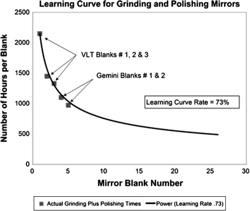
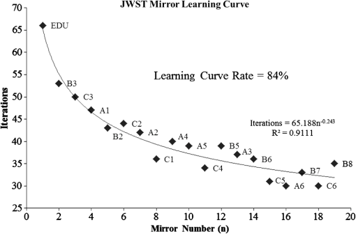
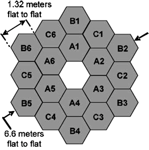
Stahl reported a single variable model of

It should be noted that in the 2005 paper, the author published the single-variable model without the multiplier because the coefficient was similar with that of the multi-variable model, but in fact it should not have matched. The reason why the single-variable diameter exponent should be lower than the multivariable diameter exponent is dominantly the effect of year of development. Year of development and aperture diameter are positively correlated ($r=0.55$, $p=0.03$), an observation that makes sense because one tends to build the largest telescope they can afford at any given time. Because technology advancement tends to reduce the cost to fabricate a telescope of a given aperture diameter, when year of development is implicitly included in the single-variable model it serves to reduce the modeled relationship between cost and diameter. When year of telescope development is made explicit as a cost variable independent of aperture diameter, the diameter exponent is larger, as was correctly published in the multivariable model presented in the Stahl 2005 paper.

3.

Learning Curve for the James Webb Space Telescope

The concept of learning curves is well known in mass-production industries, stating that each successive unit manufactured requires less labor time than the previous unit manufactured.³ Figure 2 provides evidence of a 73% learning curve for the VLT and Gemini mirrors. Note that this learning curve is estimated based on only five data points.

Fig. 2

73% learning curve for the VLT and Gemini mirrors.

Given that the James Webb Space Telescope (JWST) has manufactured 19 primary mirror segment assemblies (one Engineering Development Unit and 18 flight mirrors), it is possible to calculate an excellent estimate of the learning curve for 1.5-m-class lightweight beryllium parabolic mirrors. Based on Tinsley convergence data (private communication from Ben Gallagher), we find that JWST primary mirror segment fabrication has an excellent fit to an 84% learning curve ($R^2=91\%$) (Fig. 3). Because more mirrors were constructed for JWST than for the VLT and Gemini data in Fig. 2, the JWST data provides important support for the hypothesis that learning curves apply to optics.

Fig. 3

84% learning curve for the James Webb Space Telescope mirrors.

Further, note that the learning curve for the JWST mirrors is independent of segment prescription. Figure 4 shows the three different prescriptions of JWST (indicated on the graph with prefixes A, B, and C). The difference between these prescriptions is their off-axis distance in the primary mirror and, hence, their aspheric departure. While A segments are closest to the optical axis and thus easiest to manufacture, and B segments are furthest and thus hardest to fabricate, there appears to be no prescription-based dependency in the convergence data.

Fig. 4

Positioning of prescriptions A, B, and C on the James Webb Space Telescope.

4.

Experience Curves

The idea of learning curves can be extended to cost using experience curves, which quantify the cost savings for each successive unit produced.² Specifically, if the cost of the first unit is $C_1$, then the cost of the $n$th unit can be expressed as $C_n=C_1{n}^{-a}$, where a is chosen so that cost has the desired curve.

For the purpose of this commentary, we present an equivalent form of the segmented telescope model from Stahl 2005 in Table 2, with diameter terms cancelled out:

Table 2

Multivariable ground cost model as presented in Ref. 1.

In the 2005 paper, Stahl et al. note that the above multivariate model represents an experience curve of 80%. Here $a=0.3$ so that a doubling of production level from N to 2N results in a cost reduction of 80% between the $N$th unit and the $2N$th unit.

In order to approximate the total cost, i.e., the sum of all units, $C_N$ is integrated with respect to the unit number $n$. Thus total cost is proportional to $C_1{N}^{1-a}$.

If a ground telescope only has one prescription with $R_n$ repeats of that prescription, we can rewrite Eq. (1) as:

When there is more than one prescription, Eq. (1) shows that we multiply by the number of prescriptions. Thus ${(R_n)}^{0.7}{C}_1$ represents the total cost of each prescription, and then we multiply by the total number of prescriptions $P_n$ to find the total OTA cost. Note that the learning curve fit across prescriptions from the JWST data suggests that it may be better to ignore slight differences between prescriptions. For more information about the implications of this change in assumptions, see the next section.

5.

Improvement to the Multivariable Model

One limitation of the model is that it does not account for similarities in the manufacturing processes for prescriptions. The current framework assumes that the experience gained from manufacturing one prescription does not transfer to a second prescription; however, JWST experience shows that this is not the case. Learning from segment to segment is more important than learning from prescription to prescription. Thus it may be better to ignore differences in prescriptions altogether, and instead assume an experience curve of 80% for all of the segments combined, rather than only within prescriptions. Such a change would suggest that savings increase as the number of segments increase, even if the segments are from different prescriptions. Mathematically, distributing savings across prescriptions would mean changing the $P_n{(R_n)}^{0.7}$ term to $S^{0.7}$, where $S$ represents the total number of segments.

The model shown in Eq. (3) represents such a revised version of the model in Eq. (2) that was published in the Stahl 2005 paper. The statistical fit of the model ($R^2=91\%$, adjusted $R^2=88\%$, $\mathrm{SPE}=37\%$) is comparable to that of the original model ($R^2=95\%$, adjusted $R^2=94\%$, $\mathrm{SPE}=35\%$) given the small sample size. The dataset only contains five segmented telescopes, so it would be unwise to conclude the superiority of one model on such a small segmented sample size. Nonetheless, the JWST data suggests that experience curves apply across prescriptions.

Overall, the application of an experience curve across as opposed to within prescriptions provides only a slight change to the model. Specifically, there is a minor decrease in the segment diameter exponent (1.8 to 1.7) and in the wavelength exponent ($-0.5$ to $-0.7$). Without a larger sample size, it is impossible to accurately compare the 2005 model and the updated model. Nonetheless, intuition and experience suggest that a cost model that applies an experience curve across segments should be considered in future ground and space telescope cost models.

6.

Conclusion

After attempting to replicate the original analysis, it was found that a single variable model for ground telescope cost is given by $\text{Cost}=1.89\text{Diameter}1.40$, which differs from the model presented in the 2005 paper due to the addition of a leading multiplier. The corrected single-variable model has a lower diameter exponent for two reasons. First, more recent telescopes are less expensive per diameter than older telescopes. Second, more recent telescopes are on average larger than older telescopes because technology advancement has made larger telescopes more affordable.

The original multivariable cost model is confirmed, but only if one assumes that the learning curve does not transfer across prescriptions. For segmented telescopes, cost varies with diameter, wavelength, and year of development. Segmented mirror production benefits from an 80% learning curve. Further, cost is halved every 17 years due to developments in technology.

However, if one assumes that learning does transfer across prescriptions, then a new model is indicated. Such an assumption is warranted given results of JWST convergence. Learning from segment to segment is more important than learning between prescriptions. Low order prescription requires more material removal than the few tens of micrometers of aspheric departure difference between prescriptions. Although this assumption only results in minor changes to the model with our current dataset, the model could differ more with a larger dataset. If more data is collected, it will be worthwhile to compare the fit of the two models to see which more accurately reflects the true cost of segmented telescopes.