Correcting for focal-plane-array temperature dependence in microbolometer infrared cameras lacking thermal stabilization

Paul W. Nugent; Joseph A. Shaw; Nathan J. Pust

doi:10.1117/1.OE.52.6.061304

7 January 2013 Correcting for focal-plane-array temperature dependence in microbolometer infrared cameras lacking thermal stabilization

Paul W. Nugent, Joseph A. Shaw, Nathan J. Pust

Author Affiliations +

Optical Engineering, Vol. 52, Issue 6, 061304 (January 2013). https://doi.org/10.1117/1.OE.52.6.061304

Abstract

Advances in microbolometer detectors have led to the development of infrared cameras that operate without active temperature stabilization. The response of these cameras varies with the temperature of the camera’s focal plane array (FPA). This paper describes a method for stabilizing the camera’s response through software processing. This stabilization is based on the difference between the camera’s response at a measured temperature and at a reference temperature. This paper presents the mathematical basis for such a correction and demonstrates the resulting accuracy when applied to a commercially available long-wave infrared camera. The stabilized camera was then radiometrically calibrated so that the digital response from the camera could be related to the radiance or temperature of objects in the scene. For FPA temperature deviations within ±7.2°C changing by 0.5°C/min , this method produced a camera calibration with spatial-temporal rms variability of 0.21°C, yielding a total calibration uncertainty of 0.38°C limited primarily by the 0.32°C uncertainty in the blackbody source emissivity and temperature.

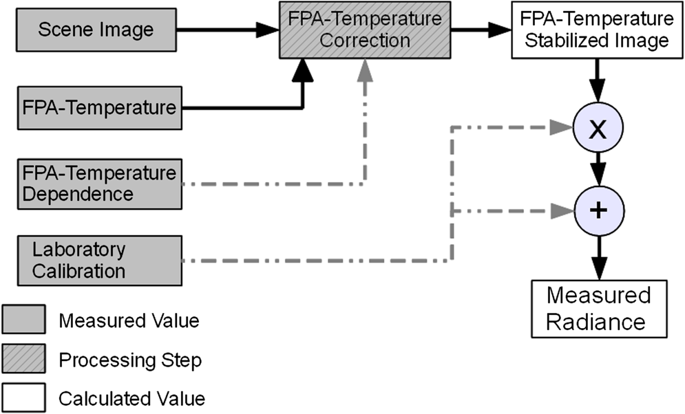
1. Introduction

Long-wave infrared (LWIR) cameras are used in a tremendously wide range of applications, ranging from environmental monitoring and industrial process control to military surveillance. The range of applications is expanding rapidly because of recent advances in uncooled microbolometer detector arrays, which enable much smaller, lighter, and lower-cost infrared imagers.¹^–³ A growing number of these applications require the camera to be calibrated radiometrically, sometimes in terms of temperature and other times in terms of radiance or a similar quantity involving optical power. For example, microbolometers provide resource-efficient radiometric remote sensing of Earth from space, but space-borne systems typically include on-board calibration sources or temperature stabilization.⁴^,⁵ However, many other applications become viable if they can be deployed without on-board calibration sources or temperature stabilization, such as sensing in agriculture and food processing,⁶ airborne remote sensing of streams and rivers,⁷ face recognition in thermal imagery,⁸ noninvasive monitoring of beehive populations,⁹ vegetation imaging to detect leaking ${CO}_{2}$ gas,¹⁰ and many others.¹¹ Yet other applications may be feasible with on-board calibration sources, but still benefit from the smaller size and lower cost associated with the use of microbolometer imagers without external calibration sources or camera temperature stabilization, such as infrared imaging polarimetry,¹² cloud imaging in climate studies,¹³ and characterizations of Earth–space optical communication paths.¹⁴

Radiometric calibration typically requires quantitatively relating the camera output to source radiance or temperature. This is most commonly done by measuring the camera’s output while it views one or more blackbody sources. Such a calibration assumes the camera’s response is time invariant, and thus a measurement of a scene taken at a later time can be calibrated to give a quantitative value. However, this assumption does not hold for a microbolometer imager with no thermo-electric cooler, whose response depends on both the focal plane array (FPA) temperature and the scene temperature. Such a camera will exhibit changes in its output that arise solely from changes in the camera temperature. Without stabilization, such cameras cannot maintain a stable radiometric calibration. For example, in a study of face recognition using thermal imagery,⁸ the authors noted that their capabilities were limited by calibration changes caused by moving the camera outdoors. This was likely a result of the calibration coefficients changing as a result of temperature fluctuations of the optics and the FPA.

Honeywell was one of the first companies to produce a thermally nonstabilized microbolometer camera, which achieved a stable response through a per-pixel calibration for every FPA temperature expected to be experienced during operation.¹ This method was mathematically intense and required the camera to be tested over all expected operating temperatures. Alternatively, there are multiple proposed methods for calibrating thermally nonstabilized infrared cameras in patent literature. For example, fourth-order polynomial curve fits have been used to relate FPA temperature to output digital number, thereby compensating for changes in FPA temperature and even temperature-induced germanium lens and window transmittance variations.¹⁵ Other methods alter the camera integration time,¹⁶ the readout bias,¹⁷ or other camera operating parameters¹⁸ to compensate for sensor response variations that result from a changing FPA temperature. Other methods determine a correction based on measurements of the camera response as a function of temperature over a wide range of conditions.¹⁹^,²⁰ At least one method relies on heat transfer models to estimate and remove the nonscene energy to determine a calibration.²¹

Most of the patent descriptions provide only the basics of the idea—with very little of the supporting mathematics—and rarely present data showing the proposed method applied to a real camera. This paper presents a technique that allows stabilization to take place through software rather than actual physical means. We present the underlying mathematics and describe a simple method of determining the coefficients required to stabilize the output of a microbolometer in the presence of camera temperature variations (we assume the FPA temperature is representative of the system). In this solution, the digital response of a camera is stabilized to the value the camera would experience at a reference FPA temperature, selected to be 25°C for this paper. This method was applied to a Photon 320 LWIR microbolometer imager (FLIR Systems), and a calibration accuracy of $\pm 0.38 ° C$ was obtained for FPA temperature deviations within $\pm 7.2 ° C$ changing by $0.5 ° C / \min$ , limited primarily by the uncertainty of the blackbody source emissivity and temperature.

2. Proposed Temperature Correction Method

The need to account for variations in FPA temperature is illustrated in this section using thermally nonstabilized microbolometer measurements of a temperature-controlled blackbody source. We placed a Photon 320 microbolometer camera and a large-area blackbody inside an environmental chamber and stepped the blackbody source temperature while cycling the chamber temperature. Specifically, the chamber air temperature was cycled with a repeating triangle ramp between 10°C and 30°C, which resulted in an oscillating FPA temperature inside the camera (Fig. 1). The blackbody source was held stable for approximately 3 h at 10°C, increased to 20°C and held constant, and so forth up to a maximum temperature of 50°C (Fig. 2). The camera viewed the blackbody source whose temperature followed the pattern in Fig. 2. The camera output (Fig. 3) had a mixed response to the blackbody source and the time-varying FPA temperature. For this particular camera, the response to the blackbody scene decreased with increasing FPA temperature.

Fig. 1

Camera focal plane array (FPA) temperature plotted versus time while the ambient air temperature inside the environmental chamber underwent a triangle ramp pattern between 10°C and 30°C.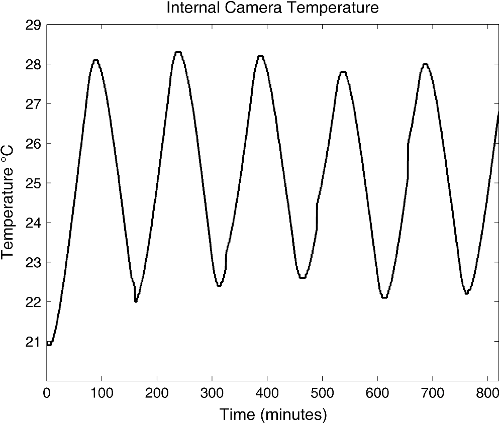

Fig. 2

Blackbody source temperature plotted versus time.

Fig. 3

Output digital number reported by the camera with a quasi-sinusoidal variation of FPA temperature (Fig. 1) while observing the blackbody source at constant but periodically stepped temperature (Fig. 2).

The method described in detail in the next section calculates the corrected digital number $r_{c}$ from the error-containing raw response $r$ , the difference between the current FPA temperature and the reference temperature, $Δ T$ , and correction coefficients $m$ and $b$ ,

Eq. (1)

r_{c} = \frac{r + b Δ T}{1 - m Δ T} .

This essentially locks the camera response to the response at the reference temperature. In practice, the reference temperature should be selected to lie at the center of the expected operating FPA-temperature range. Once the coefficients $m$ and $b$ have been determined (following procedures outlined in the next sections), the camera can be radiometrically calibrated using a standard method of viewing blackbodies at various temperatures.

The benefit of using Eq. (1) for a correction is that this equation uses only the digital values and FPA temperature from the camera, without requiring knowledge of parameters such as the camera’s spectral response, and so forth. Thus the correction for the FPA-temperature dependence can be accomplished without a full calibration of the camera. This produces a stabilized camera that subsequently can be either used in applications that require only a stable output or calibrated for applications that require radiometric data (which then requires use of the camera’s spectral response).

3. Mathematical Basis

The FPA-temperature dependence of microbolometer cameras can be modeled as a temperature-dependent response $r$ that is a linear function of a temperature-dependent responsivity or gain $G_{T}$ and a temperature-dependent dark signal or offset $D_{T}$ , which determine the digital number output by the camera in response to scene radiance $L$ :

Eq. (2)

r = G_{T} L + D_{T} .

The terms $G_{T}$ and $D_{T}$ can be written as

Eq. (3)

G_{T} = G_{m} T + G_{o}

and

Eq. (4)

D_{T} = D_{m} T + D_{o},

where

G_{m}

is an FPA temperature–dependent camera gain,

G_{o}

is a temperature-independent camera gain,

D_{m}

is a temperature-dependent dark signal, and

D_{o}

is a temperature-independent dark signal. These temperature dependences can arise from a variety of sources, including temperature dependence of the bolometer resistance, emission from the optics, emission and self-detection of the FPA, changes in the biasing resistances of the microbolometer readout circuit, and potentially other sources.¹⁵

This method assumes that all sources of temperature dependence can be related to the FPA temperature and that over a modest range the temperature dependence can be described adequately by a linear function. These assumptions hold true when the FPA and optics remain approximately equally coupled, but begin to break down when these temperatures begin to vary at different rates (e.g., with rapid or large ambient temperature changes). But with these assumptions, the terms in Eqs. (2)(3)–(4) can be combined to express the FPA temperature–dependent camera response as

Eq. (5)

r = (G_{m} T + G_{o}) L + D_{m} T + D_{o} .

If the camera views a blackbody source held at a constant temperature while the FPA temperature is changed from the reference temperature $T_{ref}$ to a different value $T_{fpa}$ , the response digital values are represented by

Eq. (6)

r_{ref} = (G_{m} T_{ref} + G_{o}) L + D_{m} T_{ref} + D_{o}

and

Eq. (7)

r_{2} = (G_{m} T_{fpa} + G_{o}) L + D_{m} T_{fpa} + D_{o} .

Because the scene radiance does not change for these two blackbody views, we can solve these equations for radiance $L$ and equate the results to obtain

Eq. (8)

\frac{r_{ref} - D_{m} T_{ref} - D_{o}}{G_{m} T_{ref} + G_{o}} = \frac{r_{2} - D_{m} T_{fpa} - D_{o}}{G_{m} T_{fpa} + G_{o}} .

We now solve for $r_{ref}$ and expand the terms over a common denominator to obtain

Eq. (9)

r_{ref} = \frac{r_{2} (G_{m} T_{ref} + G_{o}) - D_{m} T_{fpa} (G_{m} T_{ref} + G_{o}) - D_{o} (G_{m} T_{ref} + G_{o})}{G_{m} T_{fpa} + G_{o}} + \frac{D_{m} T_{ref} (G_{m} T_{fpa} + G_{o}) + D_{o} (G_{m} T_{fpa} + G_{o})}{G_{m} T_{fpa} + G_{o}} .

Next we group terms with and without $r_{2}$ :

Eq. (10)

r_{ref} = \frac{r_{2} (G_{m} T_{ref} + G_{o})}{G_{m} T_{fpa} + G_{o}} + \frac{D_{m} G_{o} - D_{o} G_{m}}{G_{m} T_{fpa} + G_{o}} (T_{ref} - T_{fpa}) .

The denominator of this equation has one term that changes with the FPA temperature and one that does not. To remove this complication, we first multiply each side by $\frac{G_{m} T_{fpa} + G_{o}}{G_{m} T_{ref} + G_{o}}$ to give

Eq. (11)

r_{ref} \frac{G_{m} T_{fpa} + G_{o}}{G_{m} T_{ref} + G_{o}} = \frac{r_{2} (G_{m} T_{ref} + G_{o})}{G_{m} T_{fpa} + G_{o}} \frac{G_{m} T_{fpa} + G_{o}}{G_{m} T_{ref} + G_{o}} + \frac{D_{m} G_{o} - D_{o} G_{m}}{G_{m} T_{fpa} + G_{o}} (T_{ref} - T_{fpa}) \frac{G_{m} T_{fpa} + G_{o}}{G_{m} T_{ref} + G_{o}},

which simplifies to

Eq. (12)

r_{ref} \frac{G_{m} T_{fpa} + G_{o}}{G_{m} T_{ref} + G_{o}} = r_{2} + \frac{D_{m} G_{o} - D_{o} G_{m}}{G_{m} T_{ref} + G_{o}} (T_{ref} - T_{fpa}),

which we further simplify to obtain

Eq. (13)

r_{ref} = \frac{r_{2} + \frac{D_{m} G_{o} - D_{o} G_{m}}{G_{m} T_{ref} + G_{o}} (T_{ref} - T_{fpa})}{\frac{G_{m} T_{fpa} + G_{o}}{G_{m} T_{ref} + G_{o}}} .

The numerator of this equation has two variables, $r_{2}$ and $(T_{ref} - T_{fpa})$ ; therefore, it will simplify calculations to put the bottom in terms of $(T_{ref} - T_{fpa})$ . This can be done by adding a term of $- G_{m} T_{ref} + G_{m} T_{ref}$ to find

Eq. (14)

r_{ref} = \frac{r_{2} + \frac{D_{m} G_{o} - D_{o} G_{m}}{G_{m} T_{ref} + G_{o}} (T_{ref} - T_{fpa})}{\frac{G_{o} + G_{m} T_{fpa} + G_{m} T_{ref} - G_{m} T_{ref}}{G_{m} T_{ref} + G_{o}}},

and then rearranging to obtain

Eq. (15)

r_{ref} = \frac{r_{2} + \frac{D_{m} G_{o} - D_{o} G_{m}}{G_{m} T_{ref} + G_{o}} (T_{ref} - T_{fpa})}{1 - \frac{G_{m}}{G_{m} T_{ref} + G_{o}} (T_{ref} - T_{fpa})} .

The two terms multiplied by $(T_{ref} - T_{fpa})$ in Eq. (15) are composed of only camera parameters and other known values that are invariant with FPA temperature changes, such as the reference temperature to which the camera response is stabilized. Therefore, we define the following two parameters:

Eq. (16)

m = \frac{G_{m}}{G_{m} T_{ref} + G_{o}}

and

Eq. (17)

b = \frac{D_{m} G_{o} - D_{o} G_{m}}{G_{m} T_{ref} + G_{o}} .

The first term, $m$ , is the temperature-dependent camera gain divided by the gain at the reference temperature. However, the value for $b$ expressed by Eq. (17) is more complicated. This value is an interaction term containing the temperature-independent and temperature-dependent dark signals and gains in the numerator and the reference-temperature gain in the denominator. If we also define

Eq. (18)

Δ T = (T_{ref} - T_{fpa}),

then Eq. (15) becomes the simple form of Eq. (1).

4. Determining the Correction Coefficients

Rewriting the reference-temperature response function from Eq. (1) as

Eq. (19)

r_{ref} - r_{2} = r_{r e f} m Δ T + b Δ T

allows us to write an equation for determining the coefficients

m

and

b

. These correction coefficients can be determined by viewing two constant-temperature blackbody scenes with radiances

L_{1}

and

L_{2}

, each with the camera at a minimum of two different temperatures,

T_{f p a 1}

and

T_{fpa 2}

. A third camera temperature

T_{fpa 3}

can be experienced while viewing the second scene, but there must be at least one common FPA temperature between the two blackbody scenes. Thus, we must consider the following responses:

r_{1}

with the camera at

T_{fpa 1}

and the blackbody at radiance

L_{1}

;

r_{2}

with the camera at

T_{fpa 2}

and the blackbody at radiance

L_{1}

;

r_{3}

with the camera at

T_{fpa 1}

and the blackbody at radiance

L_{2}

, and

r_{4}

with the camera at

T_{fpa 3}

and the blackbody at radiance

L_{2}

. The camera responses

r_{1}

and

r_{3}

are at the same FPA temperature and will be used as the references. Further, note that the responses

r_{2}

and

r_{4}

can be at the same FPA temperature, but this is not required (

T_{fpa 2}

could equal

T_{fpa 3}

). Using

T_{fpa 1}

as the reference camera temperature leads to the following differences.

Eq. (20)

Δ r_{12} = r_{1} - r_{2} and Δ T_{12} = T_{f p a 1} - T_{f p a 2},

Eq. (21)

Δ r_{34} = r_{3} - r_{4} and Δ T_{34} = T_{f p a 3} - T_{fpa 4} .

These differences can be used in Eq. (19) to write the following matrix equation:

Eq. (22)

[\begin{matrix} Δ r_{12} \\ Δ r_{34} \end{matrix}] = [\begin{matrix} r_{1} Δ T_{12} & Δ T_{12} \\ r_{3} Δ T_{34} & Δ T_{34} \end{matrix}] [\begin{matrix} m \\ b \end{matrix}],

which can be inverted to obtain

m

and

b

.

Eq. (23)

[\begin{matrix} m \\ b \end{matrix}] = {[\begin{matrix} r_{1} Δ T_{12} & Δ T_{12} \\ r_{3} Δ T_{34} & Δ T_{34} \end{matrix}]}^{- 1} [\begin{matrix} Δ r_{12} \\ Δ r_{34} \end{matrix}] .

This method is the minimal approach to deriving these coefficients, but in practice we use a large range of blackbody temperatures (for example 10°C to 60°C in steps of 10°C) and a large range of camera FPA temperatures (for example from 10°C to 30°C). This can be accomplished by placing the camera in an environmental chamber and changing the ambient temperature to drive the temperature of the camera while the blackbody remains constant, then changing the blackbody temperature and repeating the ambient temperature cycle. Doing this generates multiple reference responses, one for each combination of blackbody temperature and FPA temperature, leading to an over-determined matrix as shown in Eq. (24):

Eq. (24)

[\begin{matrix} {Δ r}_{12} \\ ⋮ \\ {Δ r}_{j k} \end{matrix}] = [\begin{matrix} r_{1} {Δ T}_{12} & {Δ T}_{12} \\ ⋮ & ⋮ \\ r_{j} {Δ T}_{j k} & {Δ T}_{j k} \end{matrix}] [\begin{matrix} m \\ b \end{matrix}] .

In such a case, a pseudo-inversion is required, and in practice the Moore–Penrose pseudo-inversion is performed. This leads to a least-squares approach that reduces noise in the estimation of m and b through Eq. (25):

Eq. (25)

[\begin{matrix} m \\ b \end{matrix}] = {[\begin{matrix} r_{1} {Δ T}_{12} & {Δ T}_{12} \\ ⋮ & ⋮ \\ r_{j} {Δ T}_{j k} & {Δ T}_{j k} \end{matrix}]}^{- 1} [\begin{matrix} Δ r_{12} \\ ⋮ \\ Δ r_{j k} \end{matrix}] .

It is important to note that this correction is determined with a unique value for every pixel. Therefore, $m$ and $b$ actually represent matrices whose dimensions match the pixel count of the FPA. In Eq. (25), $m$ and $b$ are both coefficients of first order in $Δ T$ , but sometimes it is useful to determine these coefficients as polynomials up to fourth order in $Δ T$ . However, typically only $b$ requires a higher-order description (especially in situations with widely ranging FPA temperature), whereas $m$ can remain a first-order coefficient.

Also note that the absolute temperature or radiance of the blackbody source is not needed in this temperature-stabilization method, since the blackbody is only used as a stable reference. The only requirement is for the source to remain stable during the measurements at multiple FPA temperatures. The correction uses only the measured responses and the camera FPA temperature, with no need for additional information about the camera’s spectral response or the blackbody source temperature (the camera spectral response is needed for the final radiometric calibration, but not for compensating for the FPA-temperature dependence). Nevertheless, performing this technique at two or more blackbody temperatures improves the accuracy of the coefficients in the correction. This case generates multiple reference responses, one for each blackbody temperature, leading to an overdetermined matrix, thus reducing noise in the estimation of $m$ and $b$ .

5. Application of the Method

The procedure to use this method to determine a temperature-stabilized radiometric calibration for a LWIR camera is presented in Fig. 4. First, the scene image and the FPA temperature are measured concurrently. The temperature-dependent responsivity and offset coefficients $m$ and $b$ are then used to stabilize the camera to its response at $T_{ref}$ . Finally, the stabilized response is calibrated by applying conventional gain and offset terms that were measured at or referenced to $T_{ref}$ . These gain and offset values convert the FPA temperature–stabilized data into values of integrated radiance seen by the detector. If needed, the radiance data can be converted to temperature through a lookup table created by integrating the product of the blackbody function and the camera’s spectral response function.

Fig. 4

Flow diagram for stabilization and radiometric calibration using only the FPA temperature.

Calibrating the imager in units of integrated radiance rather than temperature has advantages, most notably the nominally linear response of photo detectors with radiance or other radiometric quantities proportional to photon irradiance. This in turn allows extrapolation to very low radiance values using a calibration performed with measurements of much warmer blackbody sources.¹³^,²²^,²³ Although our technique calibrates to radiance, techniques that calibrate directly to temperature could also use the FPA temperature–stabilized data (calibrating directly in temperature requires compensating for the nonlinear relationship between the temperature of an object and its emitted radiance²⁴).

As an example of successful implementation on a microbolometer camera without thermal stabilization, we applied this method to a FLIR Photon 320 camera with a 14.25-mm lens. The camera was placed with a large-area blackbody inside an environmental chamber. Throughout the experiment, the blackbody filled the 50 deg- by 38-deg camera field of view. The blackbody was an Electro-Optical Industries CES-100 with a 15-cm aperture and microgroove surface specified with a 0.995 emissivity. The blackbody was factory calibrated with a NIST-traceable temperature uncertainty of 0.1°C. Background radiance reflected from the blackbody was removed from blackbody measurements, but was typically less than 0.75% of the observed blackbody radiance.

In this experiment, blackbody images were acquired as the source temperature was increased from 10°C to 60°C in steps of 16.7°C every 6 h. While the blackbody was held constant at each setting, the ambient temperature of the chamber was ramped in a triangle wave pattern between 15°C and 30°C in steps of 1°C every 5 min. These images were used to derive matrices of $m$ and $b$ coefficients for the stabilization Eq. (1) with $b_{i} {(Δ T)}^{i}$ terms up to order $i = 3$

The uncertainty in the resulting calibration was determined by placing the camera back inside the chamber and acquiring calibrated images of the blackbody source at different temperatures. The chamber air temperature was varied to match the outdoor air temperature measured by our weather station on a summer day and night in Bozeman, MT (ranging between 13.9°C and 26.4°C). The blackbody temperature was stepped between 10°C and 50°C and held constant for a variable length of time. The FPA temperatures and blackbody temperatures during this experiment are shown in Fig. 5. The measured data before FPA-temperature correction (black) and after correction (red) are shown in Fig. 6. Solid lines indicate the spatial mean across the FPA, while dashed lines indicate the maximum and minimum values at each instant of time (the spatial standard deviations were indistinguishably close to the mean line).

Fig. 5

Camera FPA temperature (solid line) and blackbody source temperature (dashed line) during a 24-h experiment to validate the camera stabilization method.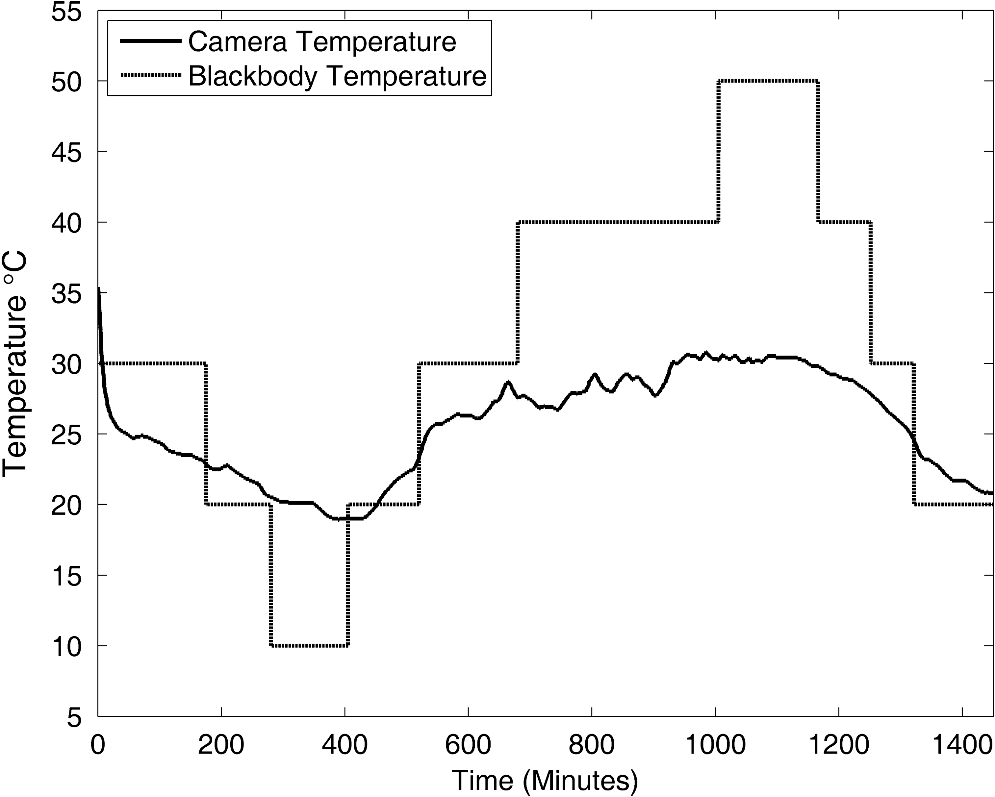

Fig. 6

Uncorrected (black) and corrected (red) digital numbers output from a microbolometer camera with a variable FPA temperature. Solid lines indicate the spatial mean across the FPA, and dashed lines indicate the maximum and minimum values across the FPA.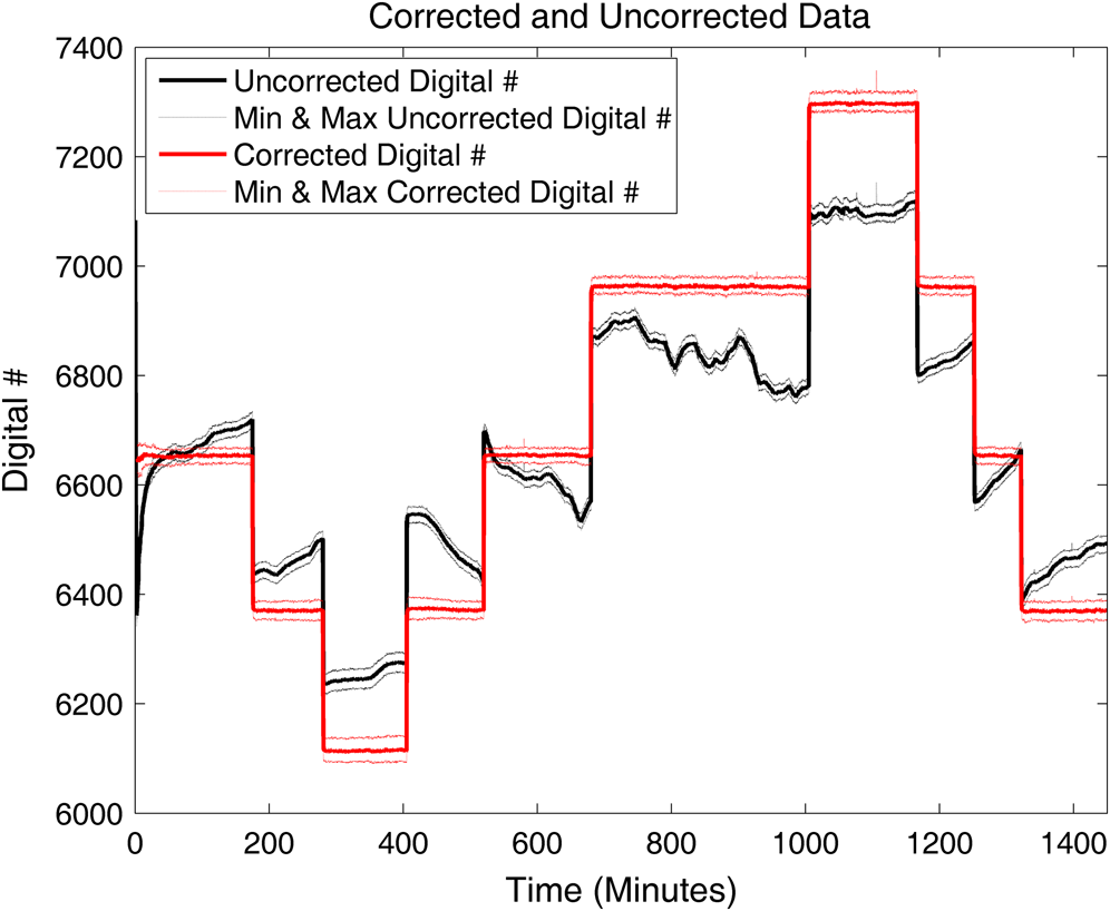

With the camera’s response stabilized as shown in Fig. 6, a conventional two-point radiometric calibration was applied using blackbody temperatures of 10°C and 60°C. Figure 7 is a time-series plot of the calibrated camera output and the blackbody source temperature for the 24-h experiment just described. The solid line indicates the spatial mean across the FPA, whereas the dashed lines indicate the maximum and minimum values across the FPA at each instant of time (the spatial standard deviations again were indistinguishably close to the mean line).

Fig. 7

Calibrated temperature readings averaged across the FPA (red solid), maximum and minimum temperature readings across the FPA (red dashed lines), and blackbody set temperatures (black dashed line).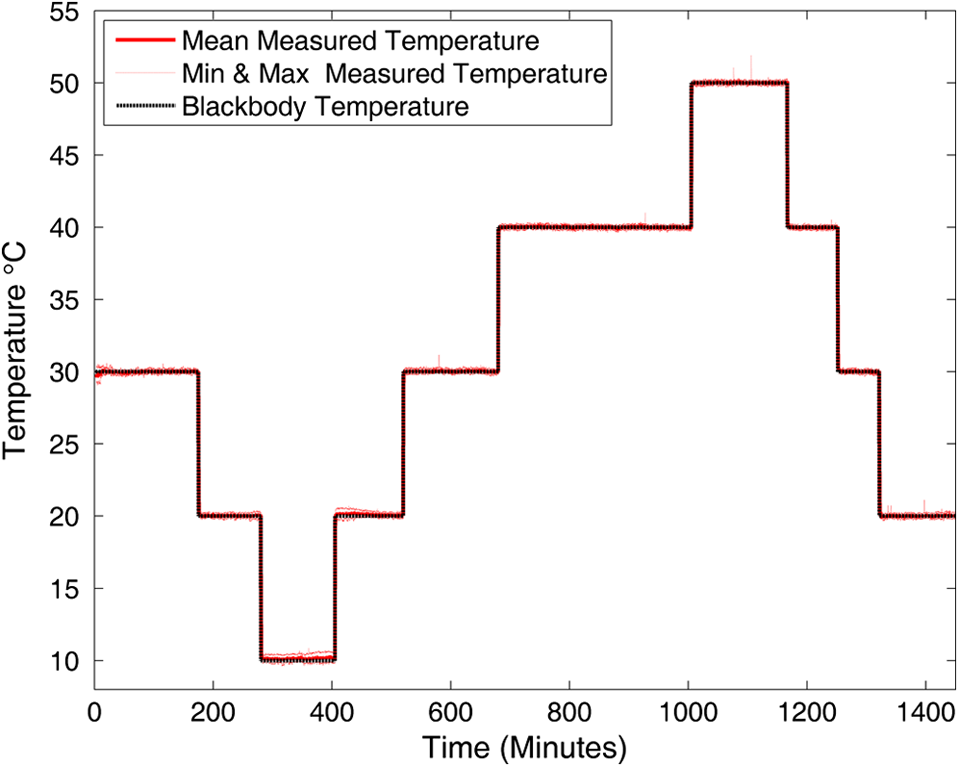

Figure 8 is a time-series plot of the difference between the blackbody source temperature and the temperature reported by the camera (from the calibrated radiance). The dashed lines in this figure indicate the expected blackbody-related calibration uncertainty of $\pm 0.32 ° C$ . This value arises from combining the blackbody temperature uncertainty ( $\pm 0.1 ° C$ ) and the blackbody emissivity uncertainty ( $0.995 \pm 0.005$ ) in the two-point calibration.²⁵ The blackbody temperature uncertainty includes blackbody spatial variation and uncertainties in readout, temperature sensor calibration, and temporal variation. The effect of the emissivity uncertainty on the calibration depends on the ambient temperature range experienced in the experiment.

Fig. 8

Difference between the calibrated camera data and the blackbody set points (red, rms $variability = 0.21 ° C$ ), along with the 0.32°C blackbody-related uncertainty (dashed black). The dashed gray lines indicate the maximum and minimum differences in each frame.

Figure 8 shows that the difference of the measurements from the blackbody set-point temperatures was within the expected uncertainty for nearly all readings. The spatial rms variation of the difference varied over time, with typical values of 0.08°C and a maximum value of 0.19°C. The temporal rms variation of this difference was 0.09°C, leading to a total spatial-temporal variability of 0.21°C. The maximum sustained difference was 0.75°C, which occurred between 300 and 450 min after the experiment began. The maximum instantaneous error was $+ 1.98 ° C$ in a single observation near 1150 min. However, this and other single-frame errors are believed to be blinking of residual bad pixels.

Figure 9 shows two histograms that provide a final illustration of the significance of this camera stabilization method, using 300 frames chosen at random times from the 24-h measurement sequence on which Figs. 5 Fig. 6 Fig. 7–8 are based. The histogram in Fig. 9(a) shows the distribution of measurement errors relative to the blackbody set point without camera stabilization, and Fig. 9(b) shows the distribution of errors with stabilization. The errors are spread over $\pm 6.25 ° C$ without stabilization and $\pm 0.3 ° C$ with stabilization. It is also interesting to note that stabilization converts the relatively uniform error distribution in Fig. 9(a) to a Gaussian-like distribution in Fig. 9(b).

Fig. 9

The histogram of the error of 300 randomly selected data files calibrated without FPA temperature compensation (a) and with FPA temperature compensation (b).

During these validation experiments, the flat field correction (FFC) of the camera was manually controlled to happen every 5 min or 0.4°C change in FPA temperature. By studying images collected before and after the FFC, it was found that the FFC had only a minor impact on the stabilized camera calibration. Just after an FFC is done, the reported temperature changed by an amount between 0.1°C and 0.25°C, decreasing when the FPA temperature was decreasing and increasing when the FPA temperature was increasing.

6. Discussion and Conclusion

This method allows for correction of the FPA temperature-dependent errors in the response of microbolometer cameras. It is unique from previously reported techniques in that it allows the stabilization to take place without a full radiometric calibration of the camera, and without requiring specific information about the camera that would be required in other techniques. In operation, the output data from the imager can be adjusted for the FPA temperature-induced errors, thus stabilizing the response of otherwise highly temperature-dependent cameras. Radiometric calibration and other data processing then can be performed on the stabilized camera response.

In many thermal infrared imaging applications, use of the technique described here can eliminate costly and space-intensive blackbody sources in field-deployed instruments, provide radiometric calibration of otherwise uncalibrated cameras, and improve the stability and accuracy of data from thermal imagers. For example, the reported technique benefits any application in which a radiometrically calibrated thermal camera is required and wherein the cost, space, or weight of an external blackbody is not desired or practical.

The reported technique was carefully implemented on a FLIR Photon 320 camera, producing a calibration with rms variability of 0.21°C, total calibration uncertainty of 0.38°C, and a maximum error of 0.75°C in a 24-h period. This calibration uncertainty is better than the value of $\pm 2 ° C$ specified for most commercial microbolometer imagers. The primary contributors to the calibration uncertainty are blackbody source emissivity and temperature. This process has produced similar results on a variety of FLIR cameras, including the Photon 320 with several wide and narrow lenses, PathFindIR, Photon 640, Tau 320, and Tau 640.

References

1.

P. W. Kruse, Uncooled Thermal Imaging, Arrays, Systems, and Applications, 64 SPIE, Bellingham, WA (2002). Google Scholar

2.

F. NiklausC. VieiderH. Jakobsen, “MEMS-based uncooled infrared bolometer arrays: a review,” Proc. SPIE, 6836 68360D (2007). http://dx.doi.org/10.1117/12.755128 PSISDG 0277-786X Google Scholar

3.

R. K. Bhanet al., “Uncooled infrared microbolometer arrays and their characterisation techniques,” Defence Sci. J., 59 (6), 580 –589 (2009). DSJOAA 0011-748X Google Scholar

4.

S. Garcia-Blancoet al., “Radiometric packaging of uncooled microbolometer FPA arrays for space applications,” Proc. SPIE, 7206 720604 (2009). http://dx.doi.org/10.1117/12.810025 PSISDG 0277-786X Google Scholar

5.

H. Geoffrayet al., “Evaluation of a COTS microbolometers FPA to space environments,” Proc. SPIE, 7826 78261U (2010). http://dx.doi.org/10.1117/12.869726 PSISDG 0277-786X Google Scholar

6.

R. VadivambalD. S. Jayas, “Applications of thermal imaging in agriculture and food industry: a review,” Food Bioprocess. Technol., 4 (2), 186 –199 (2011). http://dx.doi.org/10.1007/s11947-010-0333-5 FBTOAV 1935-5130 Google Scholar

7.

S. RayneG. S. Henderson, “Airborne thermal infrared remote sensing of stream and riparian temperatures in the Nicola River watershed, British Columbia, Canada,” J. Environ. Hydrol., 12 1 –11 (2004). Google Scholar

8.

D. A. SocolinskyA. SelingerJ. D. Neuheisel, “Face recognition with visible and thermal infrared imagery,” Comp. Vis. Image Understand., 91 (1–2), 72 –114 (2003). http://dx.doi.org/10.1016/S1077-3142(03)00075-4 CVIUF4 1077-3142 Google Scholar

9.

J. A. Shawet al., “Long-wave infrared imaging for non-invasive beehive population assessment,” Opt. Express, 19 (1), 399 –408 (2011). http://dx.doi.org/10.1364/OE.19.000399 OPEXFF 1094-4087 Google Scholar

10.

J. E. Johnsonet al., “Long-wave infrared imaging of vegetation for detecting leaking ${CO}_{2}$ gas,” J. Appl. Rem. Sens., 6 (1), 063612 (2012). http://dx.doi.org/10.1117/1.JRS.6.063612 Google Scholar

11.

M. VollmerK.-P. Möllmann, Infrared Thermal Imaging, Wiley-VCH, Weinheim, Germany (2010). Google Scholar

12.

M. W. KudenovJ. L. PezzanitiG. R. Gerhart, “Microbolometer-infrared imaging Stokes polarimeter,” Opt. Eng., 48 (6), 063201 (2009). http://dx.doi.org/10.1117/1.3156844 OPEGAR 0091-3286 Google Scholar

13.

J. Shawet al., “Radiometric cloud imaging with an uncooled microbolometer thermal infrared camera,” Opt. Express, 13 (15), 5807 –5817 (2005). http://dx.doi.org/10.1364/OPEX.13.005807 OPEXFF 1094-4087 Google Scholar

14.

P. W. NugentJ. A. ShawS. Piazzolla, “Infrared cloud imaging in support of Earth-space optical communication,” Opt. Express, 17 (10), 7862 –7872 (2009). http://dx.doi.org/10.1364/OE.17.007862 OPEXFF 1094-4087 Google Scholar

15.

T. HoelterB. Meyer, “The challenges of using an uncooled microbolometer array in a thermographic application,” (2012) http://www.dtic.mil/cgi-bin/GetTRDoc?Location=U2&doc=GetTRDoc.pdf&AD=ADA399432 September ). 2012). Google Scholar

16.

WandM. A.et al., “Ambient temperature micro-bolometer control, calibration, and operation,” U.S. Patent 6267501 (2001).

17.

AndersonS. M.McManusT., “Microbolometer focal plane array with temperature compensated bias,” U.S. Patent 7105818 (2006).

18.

ButlerN. R., “Method and apparatus for compensating radiation sensor for temperature variations of the sensor,” U.S. Patent 6740909 (2004).

19.

HowardP. E., “Infrared sensor temperature compensated response and offset correction,” U.S. Patent 6433333 (2002).

20.

KaufmanC. S.CarsonR. S.HornbackW. B., “Method and apparatus for temperature compensation of an uncooled focal plane array,” U.S. Patent 6476292 (2002).

21.

GrimbergE., “Radiometry using an uncooled microbolometer detector,” U.S. Patent application US2008/0210872 (2008).

22.

Y. Hanet al., “Infrared spectral radiance measurements in the tropical Pacific atmosphere,” J. Geophys. Res., 102 (D4), 4353 –4356 (1997). http://dx.doi.org/10.1029/96JD03717 JGREA2 0148-0227 Google Scholar

23.

R. O. Knutesonet al., “Atmospheric emitted radiance interferometer. Part II: instrument performance,” J. Atmos. Ocean. Technol., 21 (12), 1777 –1789 (2004). http://dx.doi.org/10.1175/JTECH-1663.1 JAOTES 0739-0572 Google Scholar

24.

J. A. ShawL. S. Fedor, “Improved calibration of infrared radiometers for cloud temperature remote sensing,” Opt. Eng., 32 (5), 1002 –1010 (1993). http://dx.doi.org/10.1117/12.133232 OPEGAR 0091-3286 Google Scholar

25.

C. L. WyattV. PrivalskyR. Datla, “Recommended practice; symbols, terms, units and uncertainty analysis for radiometric sensor calibration,” NIST Handbook 152, U.S. Government Printing Office, Washington, DC (1998). Google Scholar

Biography

Paul W. Nugent is a research engineer with the Electrical and Computer Engineering Department at Montana State University and president of NWB Sensors Inc. in Bozeman, Montana. He received his MS and BS degrees in electrical engineering from Montana State University. His research activities include radiometric thermal imaging and optical remote sensing.

Joseph A. Shaw is the director of the Optical Technology Center, professor of electrical and computer engineering, and affiliate professor of physics at Montana State University in Bozeman, Montana. He received PhD and MS degrees in optical sciences from the University of Arizona, an MS degree in electrical engineering from the University of Utah, and a BS degree in electrical engineering from the University of Alaska–Fairbanks. He conducts research on the development and application of radiometric, polarimetric, and laser-based optical remote sensing systems. He is a Fellow of the OSA and SPIE.

Nathan J. Pust is a research engineer working at Montana State University. He received bachelor’s degrees in electrical engineering and computer engineering from Montana State University in 2002, and his PhD in electrical engineering from Montana State University in 2007.

CC BY: © The Authors. Published by SPIE under a Creative Commons Attribution 4.0 Unported License. Distribution or reproduction of this work in whole or in part requires full attribution of the original publication, including its DOI.

Citation Download Citation

Paul W. Nugent, Joseph A. Shaw, and Nathan J. Pust "Correcting for focal-plane-array temperature dependence in microbolometer infrared cameras lacking thermal stabilization," Optical Engineering 52(6), 061304 (7 January 2013). https://doi.org/10.1117/1.OE.52.6.061304

Published: 7 January 2013

Access the abstract

JOURNAL ARTICLE
8 PAGES

DOWNLOAD PAPER SAVE TO MY LIBRARY

GET CITATION

CITATIONS

Cited by 60 scholarly publications.

Explore citations on Lens.org

KEYWORDS

Cameras

Staring arrays

Black bodies

Calibration

Temperature metrology

Microbolometers

Infrared cameras

1.

Introduction

2.

Proposed Temperature Correction Method

Fig. 1

Fig. 2

Fig. 3

Eq. (1)

3.

Mathematical Basis

Eq. (2)

Eq. (3)

Eq. (4)

Eq. (5)

Eq. (6)

Eq. (7)

Eq. (8)

Eq. (9)

Eq. (10)

Eq. (11)

Eq. (12)

Eq. (13)

Eq. (14)

Eq. (15)

Eq. (16)

Eq. (17)

Eq. (18)

4.

Determining the Correction Coefficients

Eq. (19)

Eq. (20)

Eq. (21)

Eq. (22)

Eq. (23)

Eq. (24)

Eq. (25)

5.

Application of the Method

Fig. 4

Fig. 5

Fig. 6

Fig. 7

Fig. 8

Fig. 9

6.

Discussion and Conclusion

References

Biography

Show All Keywords

Keywords/Phrases

Search In:

Publication Years