Stereo matching algorithm based on illumination normal similarity and adaptive support weight

Kai Gao; He-xin Chen; Yan Zhao; Ying-nan Geng; Gang Wang

doi:10.1117/1.OE.52.2.027201

1 February 2013 Stereo matching algorithm based on illumination normal similarity and adaptive support weight

Kai Gao, He-xin Chen, Yan Zhao, Ying-nan Geng, Gang Wang

Author Affiliations +

Optical Engineering, Vol. 52, Issue 2, 027201 (February 2013). https://doi.org/10.1117/1.OE.52.2.027201

Abstract

For the purpose of representing the feature of the gray image, illumination normal of pixels in a two-dimensional gray image plane is proposed, which can reflect the high-frequency information of the gray image. In order to get an accurate dense disparity map based on the adaptive support weight (ASW) approach in RGB vector space, a matching algorithm is proposed that combines the illumination normal similarity, gradient similarity, color similarity, and Euclidean distance similarity to compute the corresponding support weights and dissimilarity measurements. After testing by the Middlebury stereo benchmark, the result of the proposed algorithm shows more accurate disparity than many state-of-the-art stereo matching algorithms.

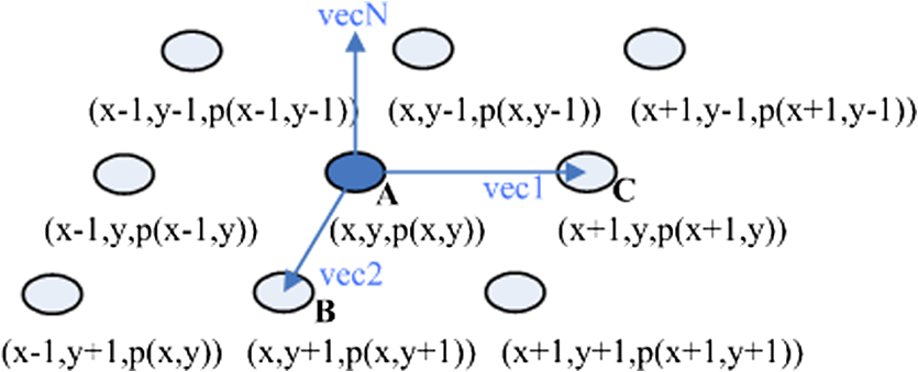
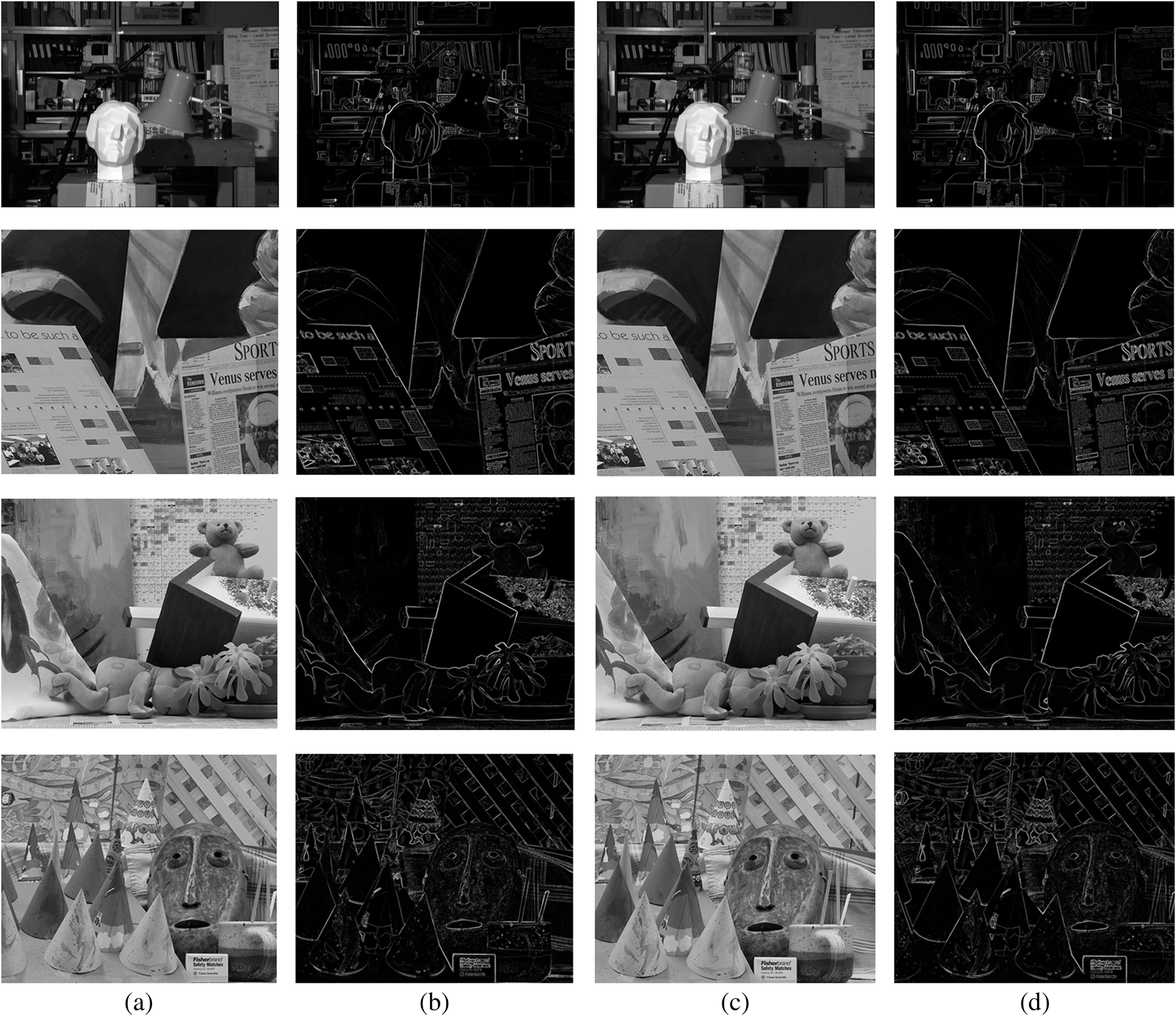
1. Introduction

Dense stereo matching is one of the most challenging problems in the field of computer vision. It is an important requirement for many applications, such as three-dimensional (3-D) reconstruction and virtual view synthesis. Generally, the purpose of stereo matching is to find the corresponding pixels between the stereo image pairs captured by two or more cameras in the same scene, and get the disparity map composed by the coordinate difference of corresponding pixels in the stereo image pair.

There are plenty of algorithms available to solve the dense stereo problem, the choice of which depends on whether you want to get the area-based solution by a global method or local method. Stereo matching algorithms can be classified as either global or local. The typical global algorithms, such as graph cuts,¹ belief propagation,²^,³ and dynamic programming,⁴^,⁵ can generate a dense disparity map precisely based on global energy function and suitable constraints. However, graph cuts and belief propagation usually consume a great deal of time and memory, and dynamic programming needs specific constraints at different times. Local matching algorithms are known for their simplicity and efficiency, and they also can achieve disparity more accurately. The basic idea of local matching is to estimate the disparity of a pixel in the target image by correlating a support window around the pixel with a similar support window in the reference image. One of the typical local matching algorithms is adaptive support weight (ASW), proposed by Yoon.⁶ The method in Ref. 6 adopts the fixed-size square windows and allocates a support weight to each pixel in the window according to pixel color and position similarities. The disparity map generated by Ref. 6 can get perfect effects similar to that obtained by global algorithms. The gradient information can indicate the variation between neighboring pixels and the structure of the information,⁷ as well as decreasing the noise presented in the disparity map more. The method that uses the gradient similarity and local ASW to compute the disparity is proposed.⁸ Considering that the information will be lost when converting the stereo images from RGB vector space to the CIELab color space, the ASW approach in RGB vector space is proposed.⁹ The gradient similarity is used to compute the support weight in Ref. 9. However, the difficulties in stereo matching are still at the boundaries of objects and ﬁne texture area, which can be reflected by the high-frequency information. In this paper, we propose to utilize the illumination normal similarity of the two-dimensional (2-D) gray image to compute the support weight based on the ASW in RGB vector space. The experimental results prove that the proposed method can improve the accuracy of the disparity map.

This paper is organized as follows. Section 2 gives the definition of illumination normal in the image space. Section 3 provides a specific explanation for the proposed method. In Sec. 4, experimental results of the proposed method are compared to that of other methods. Conclusions and future work are provided in Sec. 5.

2. Illumination Normal of Pixels in a 2-D Image Plane

A normal vector almost exists for each point of the object in 3-D space. Given a 2-D gray image, the gray value of every pixel can reflect the illumination information of the object. In order to obtain the illumination normal vector of pixels in a 2-D image, each pixel of the image is regarded as a point in 3-D space. This can be expressed as $P [x, y, p (x, y)]$ , where $x$ and $y$ are the horizontal and vertical coordinates, respectively, and $p (x, y)$ is the pixel value at the position $(x, y)$ .

The current point and the points located below and to the right of it are used to compute its normal vector. Figure 1 illustrates how the illumination normal vector is calculated. Point $A$ is the current point, $B$ and $C$ are the neighboring points used to compute the normal vector of point $A$ . The 3-D vectors from $A$ to $C$ and from $A$ to $B$ are computed as follows:

Eq. (1)

v e c 1 = P (C) - P (A) = P [x + 1, y, p (x + 1, y)] - P [x, y, p (x, y)]

Eq. (2)

v e c 2 = P (B) - P (A) = P [x, y + 1, p (x, y + 1)] - P [x, y, p (x, y)] .

Fig. 1

The illustration of calculating the illumination normal vector.

The illumination normal vector of point $A$ is obtained by the cross-product of $v e c 1$ and $v e c 2$ :

Eq. (3)

v e c N (A) = v e c 1 \times v e c 2 = [{v e c N}_{x} (A), v e c N_{y} (A), v e c N_{z} (A)] .

Normalize the illumination normal vector of point $A$ :

Eq. (4)

normal (A) = n [n_{x} (A), n_{y} (A), n_{z} (A)],

where

Eq. (5)

n_{x} (A) = \frac{v e c N_{x} (A)}{\sqrt{{[v e c N_{x} (A)]}^{2} + {[v e c N_{y} (A)]}^{2} + {[v e c N_{z} (A)]}^{2}}}

Eq. (6)

n_{y} (A) = \frac{v e c N_{y} (A)}{\sqrt{{[v e c N_{x} (A)]}^{2} + {[v e c N_{y} (A)]}^{2} + {[v e c N_{z} (A)]}^{2}}}

Eq. (7)

n_{z} (A) = \frac{v e c N_{z} (A)}{\sqrt{{[v e c N_{x} (A)]}^{2} + {[v e c N_{y} (A)]}^{2} + {[v e c N_{z} (A)]}^{2}}} .

The modulus images of the illumination normal vector of the image pairs, which are used to analyze the illumination normal similarity of the image pairs, are shown in Fig. 2. The features of the illumination normal vector in Fig. 2(b) and 2(d) reflect the high-frequency information of the gray image pairs. The high-frequency information reflects some small-scale details of the image, which is useful for searching the matching pixels in the stereo pair. In this paper, the character mentioned above is utilized, and the illumination normal similarity of the gray image is combined into the ASW method to compute the weights in the support window.

Fig. 2

The analysis of illumination normal vectors of image pairs. (a) left image (gray); (b) the modulus image of the illumination normal vector of the left image (gray); (c) right image (gray); (d) the modulus image of the illumination normal vector of the right image (gray).

3. Proposed Algorithm

To assign the support weight more accurately for each pixel in the support window, the similarity measurements are considered. Geng et al.⁹ adds the gradient similarity in RGB vector space to the gestalt group proposed by Yoon.⁶ Here, we propose to compute the support weight by a number of multi-similarity measurements, including color similarity, Euclidean distance similarity, gradient similarity, and illumination normal similarity. The support weight of a pixel in a support window can be expressed by

Eq. (8)

w (\vec{p}, \vec{q}) = \exp (- \frac{{Δ c}_{\vec{p} \vec{q}}}{τ_{c}}) \cdot \exp (- \frac{{Δ dis}_{\vec{p} \vec{q}}}{τ_{d}}) \cdot \exp (- \frac{{Δ grad}_{\vec{p} \vec{q}}}{τ_{g}}) \cdot \exp (- \frac{{Δ n}_{p q}}{τ_{n}}),

where

\vec{p}

,

\vec{q}

are the pixels in the reference image, which have the RGB components;

\vec{q}

is the pixel in the support window centered at

\vec{p}

;

{Δ c}_{\vec{p} \vec{q}}

,

{Δ dis}_{\vec{p} \vec{q}}

, and

{Δ grad}_{\vec{p} \vec{q}}

are the color difference, spatial distance, and gradient difference between pixel

\vec{p} (x, y) = {p_{R}, p_{G}, p_{B}}

and

\vec{q} (x, y) = {q_{R}, q_{G}, q_{B}}

, respectively;

{Δ n}_{\vec{p} \vec{q}}

is the illumination normal difference between

p_{Gray}

and

q_{Gray}

;

p_{Gray}

and

q_{Gray}

are the gray values of

\vec{p}

and

\vec{q}

, respectively; and

τ_{c}

,

τ_{d}

,

τ_{g}

and

τ_{n}

are all constant.

{Δ c}_{\vec{p} \vec{q}}

,

{Δ dis}_{\vec{p} \vec{q}}

,

{Δ grad}_{\vec{p} \vec{q}}

and

{Δ n}_{p q}

are calculated by

Eq. (9)

{Δ c}_{\vec{p} \vec{q}} = {‖ \vec{p} - \vec{q} ‖}_{2} = \sqrt{{(p_{R} - q_{R})}^{2} + {(p_{G} - q_{G})}^{2} + {(p_{B} - q_{B})}^{2}}

Eq. (10)

{Δ dis}_{\vec{p} \vec{q}} = {‖ {dis}_{\vec{p}} - {dis}_{\vec{q}} ‖}_{2} = \sqrt{{(x_{\vec{p}} - x_{\vec{q}})}^{2} + {(y_{\vec{p}} - y_{\vec{q}})}^{2}}

Eq. (11)

{Δ grad}_{\vec{p} \vec{q}} = {Δ grad x}_{\vec{p} \vec{q}} + {Δ grad y}_{\vec{p} \vec{q}} = {‖ {grad x}_{\vec{p}} - {grad x}_{\vec{q}} ‖}_{2} + {‖ {grad y}_{\vec{p}} - {grad y}_{\vec{q}} ‖}_{2}

Eq. (12)

{Δ n}_{p q} = {‖ n (p) - n (q) ‖}_{2} = \sqrt{{[n_{x} (p) - n_{x} (q)]}^{2} + {[n_{y} (p) - n_{y} (q)]}^{2} + {[n_{z} (p) - n_{z} (q)]}^{2}} .

The weights calculated for the pixels in the window between the reference image and the target image are combined in the aggregation step. The dissimilarity $E$ can be expressed by

Eq. (13)

E (\vec{p}, {\vec{p}}_{d}) = \frac{1}{N} \sum_{\vec{q} \in N_{\vec{p}}, {\vec{q}}_{d} \in N_{{\vec{p}}_{d}}} e_{matching} (\vec{q}, {\vec{q}}_{d}) \cdot w (\vec{p}, \vec{q}),

where

{\vec{p}}_{d}

and

{\vec{q}}_{d}

are the corresponding pixels in the target image for

\vec{p}

and

\vec{q}

with the disparity

d

;

N_{\vec{p}}

and

N_{{\vec{p}}_{d}}

are the support windows centered at

\vec{p}

and

{\vec{p}}_{d}

, respectively; and

e_{matching} (\vec{q}, {\vec{q}}_{d})

is the pixel-based matching cost between

\vec{q}

and

{\vec{q}}_{d}

, which is obtained by

Eq. (14)

e_{matching} (\vec{q}, {\vec{q}}_{d}) = e_{c} (\vec{q}, {\vec{q}}_{d}) \cdot e_{dis} (\vec{q}, {\vec{q}}_{d}) \cdot e_{n} (q, q_{d}) .

Here,

e_{c} (\vec{q}, {\vec{q}}_{d})

is the color difference,

e_{dis} (\vec{q}, {\vec{q}}_{d})

is the gradient difference, and

e_{n} (\vec{q}, {\vec{q}}_{d})

is the illumination normal difference, as follows:

Eq. (15)

e_{c} (\vec{q}, {\vec{q}}_{d}) = \exp (- \frac{{Δ c}_{\vec{q} {\vec{q}}_{d}}}{λ_{c}})

Eq. (16)

e_{grad} (\vec{q}, {\vec{q}}_{d}) = \exp (- \frac{{Δ grad x}_{\vec{q} {\vec{q}}_{d}}}{λ_{grad x}} - \frac{{Δ grad y}_{\vec{q} {\vec{q}}_{d}}}{λ_{grad y}})

Eq. (17)

e_{n} (q, q_{d}) = \exp (- \frac{{Δ n}_{q, q_{d}}}{λ_{n}}),

where

{Δ c}_{\vec{q} {\vec{q}}_{d}}

,

{Δ grad x}_{\vec{q} {\vec{q}}_{d}}

,

{Δ grad y}_{\vec{q} {\vec{q}}_{d}}

, and

{Δ n}_{q, q_{d}}

are obtained by Eqs. (9)–(12), and

λ_{c}

,

λ_{grad x}

,

λ_{grad y}

, and

λ_{n}

are constant.

Find the best disparity of pixel $\vec{p}$ by maximizing the dissimilarity function $E (\vec{p}, {\vec{p}}_{d})$ :

Eq. (18)

d_{\vec{p}} = \underset{d \in D}{arg max} E (\vec{p}, {\vec{p}}_{d}),

where

D = {d_{\min, \dots,} d_{\max}}

is the search range of possible disparities, which is variable for different image pairs.

In order to refine the disparity, the consistency check is used to detect matching errors, as follows:

Eq. (19)

D_{L} (x, y) = - d_{R} [x - d_{L} (x, y), y],

where

d_{L} (x, y)

is the disparity of the pixels regarding the left image as the reference image and

d_{R} (x, y)

is the disparity of the pixels regarding the right image as the reference image. Here,

d_{L} (x, y)

and

d_{R} (x, y)

are computed separately. The pixels that fail during the consistency check are classified as bad. The support weight for each neighboring pixel in the fixed-size support window centered on the bad pixel is recomputed using the proposed method. The disparity of the pixel with the largest support weight when recomputed is considered to be the disparity of the bad pixel.

4. Experimental Results

4.1.

Performance Comparison

The stereo image pairs “tsukuba,” “venus,” “teddy,” and “cones,” which are provided by the Middlebury stereo benchmark, were used in our experiments. The size of the support window was fixed at $35 \times 35 pixels$ , and the constants $τ_{c} = 30$ , $λ_{c} = 40$ , $τ_{d} = 10$ , $λ_{grad x} = 20$ , $λ_{grad y} = 10$ , $τ_{g} = 30$ ,⁹ $τ_{n} = 40$ , and $λ_{n} = 1$ were fixed for all the test stereo image pairs. To evaluate the proposed algorithm, we obtained the ground truth provided by Scharstein and Szeliski¹⁰ and the disparity maps of the ASW method by Yoon⁶ in the Middlebury stereo benchmark. The subjective quality comparison of the disparity maps is shown in Fig. 3. Figure 3(a) and 3(b) are the color image and the ground truth, respectively; while Fig. 3(c), 3(e), 3(g) and Fig. 3(d), 3(f), and 3(h) are the disparity maps and the bad-pixel images of disparity maps produced by our algorithm, ASW,⁶ and ASW-RGB,⁹ respectively. The error threshold $T h$ in our experiment was 0.5. We found that the smaller the area of gray and black was, the more accurate the disparity map was. Figure 3(d), 3(f), and 3(h) shows that the disparity map of our algorithm is more accurate than those of ASW⁶ and ASW-RGB.⁹

Fig. 3

The comparison of results. (a) Left image. (b) Ground truth. (c) Disparity map generated by our algorithm. (d) Bad-pixel image of our algorithm. (e) Disparity map generated by the ASW approach.⁶ (f) Bad-pixel image of the ASW approach.⁶ (g) Disparity map generated by the ASW-RGB approach.⁹ (h) Bad-pixel image of the ASW-RGB approach.⁹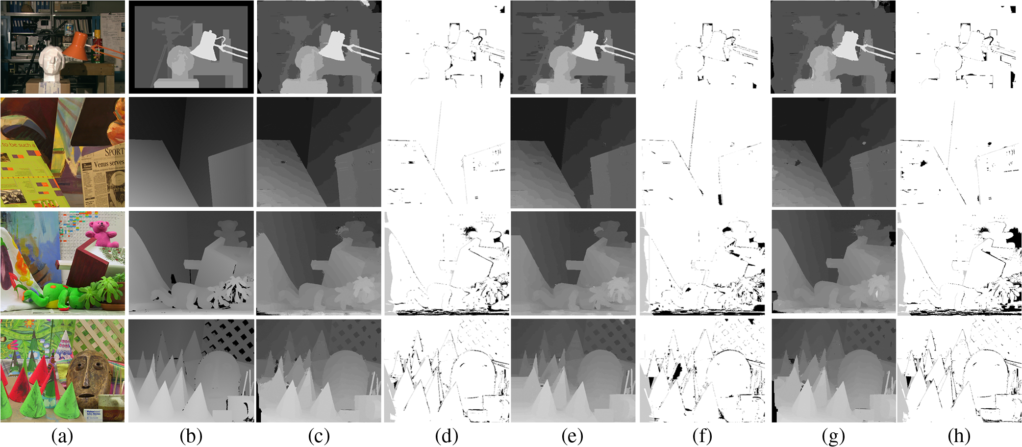

In order to measure the objective quality of the disparity map, the Middlebury stereo benchmark provides the quality metrics to evaluate the generated disparity map, which can be separated into three parts: all pixels (“all”), nonoccluded regions (“nonocc”), and pixels near depth discontinuities (“disc”). When the absolute difference between generated disparity and ground truth is less than $T h$ , the generated disparity value can be considered correct. Tables 1 and 2 show two cases of $T h = 1$ and $T h = 0.5$ . To evaluate the proposed algorithm objectively, it is compared to the results of the other local matching ASW methods.⁶^,⁸^,⁹^,¹¹^–¹³ The comparison of results is shown in Tables 1 and 2, and the results of the proposed algorithm (ASW-MS) improve the matching accuracy by different degrees.

Table 1

Performance comparison of the proposed method with the Middlebury stereo benchmark (error threshold: 1.0).

Algorithm	Tsukuba			Venus			Teddy			Cones			Average percent of bad pixels
Algorithm	Nonocc	All	Disc	Nonocc	All	Disc	Nonocc	All	Disc	Nonocc	All	Disc	Average percent of bad pixels
ASW-MS (proposed)	2.03	2.63	8.50	0.50	0.96	2.17	6.57	11.9	17.1	2.96	8.55	7.93	5.98
AdaptDispCalib¹¹	1.19	1.42	6.15	0.23	0.34	2.50	7.80	13.6	17.3	3.62	9.33	9.72	6.10
VSW¹²	1.62	1.88	6.98	0.47	0.81	3.40	8.67	13.3	18.0	3.37	9.87	9.77	6.29
GradAdaptWgt⁸	2.26	2.63	8.99	0.99	1.39	4.92	8.00	13.1	18.2	2.61	7.67	7.43	6.55
Adaptweight⁶	1.38	1.85	6.90	0.71	1.19	6.13	7.88	13.3	18.6	3.97	9.79	8.26	6.67
ASW-RGB⁹	2.56	3.19	9.89	0.91	1.56	4.46	8.48	13.5	19.2	3.32	8.91	8.72	7.06
BioPsyASW¹³	3.62	5.52	14.6	3.15	4.20	20.4	11.5	18.2	23.2	4.93	13.0	11.7	11.2

Table 2

Performance comparison of the proposed method with the Middlebury stereo benchmark (error threshold: 0.5).

Algorithm	Tsukuba			Venus			Teddy			Cones			Average percent of bad pixels
Algorithm	Nonocc	All	Disc	Nonocc	All	Disc	Nonocc	All	Disc	Nonocc	All	Disc	Average percent of bad pixels
ASW-MS (proposed)	9.23	9.98	15.3	6.14	6.75	11.1	12.2	18.8	27.1	7.80	13.7	15.2	12.8
GradAdaptWgt⁸	7.67	8.25	15.0	7.51	8.05	12.3	13.5	19.6	28.5	7.34	13.0	14.8	13.0
ASW-RGB⁹	9.82	10.6	16.1	7.94	8.70	13.4	14.3	20.5	29.5	8.16	14.0	15.8	14.1
VSW¹²	19.2	19.5	18.5	8.17	8.65	13.2	17.4	23.2	31.4	13.1	18.3	20.4	17.6
AdaptDispCalib¹¹	24.6	24.7	21.3	7.14	7.56	15.0	18.8	25.2	29.7	9.21	15.1	16.7	17.9
Adaptweight⁶	18.1	18.8	18.6	7.77	8.40	15.8	17.6	23.9	34.0	14.0	19.7	20.6	18.1
BioPsyASW¹³	22.9	24.4	24.1	9.69	10.8	24.5	18.5	26.1	34.5	12.6	20.2	22.3	20.9

4.2.

Influence of the Illumination Normal

In order to analyze the influence of the illumination normal in the algorithm, the experiment with illumination normal (ASW-MS) and without illumination normal (ASW-MS-outN) were tested. The comparison results are shown in Tables 3 and 4. The data in these tables are the percentages of the bad pixels. For a more accurate disparity map, the smallest percentage of bad pixels is needed. Tables 3 and 4 show that having the illumination normal similarity can get a more accurate result than being without the illumination normal similarity.

Table 3

Performance comparison of the proposed method with and without illumination normal in the Middlebury stereo benchmark (error threshold: 1.0).

Algorithm	Tsukuba			Venus			Teddy			Cones			Average percent of bad pixels
Algorithm	Nonocc	All	Disc	Nonocc	All	Disc	Nonocc	All	Disc	Nonocc	All	Disc	Average percent of bad pixels
ASW-MS	2.03	2.63	8.50	0.50	0.96	2.17	6.57	11.9	17.1	2.96	8.55	7.93	5.98
ASW-MS-outN	2.48	3.04	9.53	1.03	1.73	4.84	8.13	13.2	19.1	3.22	8.92	8.55	6.98

Table 4

Performance comparison of the proposed method with and without illumination normal in the Middlebury stereo benchmark (error threshold: 0.5).

Algorithm	Tsukuba			Venus			Teddy			Cones			Average percent of bad pixels
Algorithm	Nonocc	All	Disc	Nonocc	All	Disc	Nonocc	All	Disc	Nonocc	All	Disc	Average percent of bad pixels
ASW-MS	9.23	9.98	15.3	6.14	6.75	11.1	12.2	18.8	27.1	7.80	13.7	15.2	12.8
ASW-MS-outN	13.1	13.7	17.3	8.22	8.99	13.2	14.1	20.4	29.6	7.94	13.9	15.6	14.7

4.3.

Performance Analysis of the Proposed Method with Different Sizes of the Support Window

The size ( $35 \times 35$ ) of the support window of the proposed method is the same as that of Refs. 8, 9, and 12. In order to compare our results to Refs. 6 and 11, which used different sizes of support window, we tested the proposed method using the same sizes of support window as those studies used. The other relevant constants in the algorithm are the same as in the case of the $35 \times 35$ support window. The size of the support window in our algorithm is odd and the central point of the window is a pixel, while the size ( $48 \times 48$ ) of the support window in Ref. 13 is even and there is no pixel at the central point of the window, so the comparison result between Ref. 13 and the proposed algorithm is not listed.

Tables 5 and 6 show the comparative results between the proposed method and that of Refs. 6 and 11 with the size ( $33 \times 33$ , $21 \times 21$ ) of the support window and error threshold 1.0 and 0.5, respectively. The results show that the size of the support window can affect the matching precision when the other relevant constants are fixed in the algorithm. When the error threshold is 1.0, the average percentage of bad pixels of the proposed method is less than that of other references except Ref. 11. For error threshold 0.5, however, all results of the proposed method are better than those of Refs. 6 and 11.

Table 5

Performance comparison of the proposed method with Refs. 6 and 11 in terms of the size (33×33, 21×21) of the support window in the Middlebury stereo benchmark (error threshold: 1.0).

Algorithm	Tsukuba			Venus			Teddy			Cones			Average percent of bad pixels
Algorithm	Nonocc	All	Disc	Nonocc	All	Disc	Nonocc	All	Disc	Nonocc	All	Disc	Average percent of bad pixels
Adaptweight⁶ ( $33 \times 33$ )	1.38	1.85	6.90	0.71	1.19	6.13	7.88	13.3	18.6	3.97	9.79	8.26	6.67
ASW-MS ( $33 \times 33$ )	2.04	2.65	8.47	0.54	1.00	2.16	6.55	11.9	17.0	2.91	8.54	7.82	5.96
AdaptDispCalib¹¹ ( $21 \times 21$ )	1.19	1.42	6.15	0.23	0.34	2.50	7.80	13.6	17.3	3.62	9.33	9.72	6.10
ASW-MS ( $21 \times 21$ )	2.65	3.32	7.68	0.84	1.40	2.88	6.93	12.4	16.9	2.65	8.46	7.23	6.11

Table 6

Performance Comparison of the proposed method with Refs. 6 and 11 in terms of the size (33×33, 21×21) of the support window in the Middlebury stereo benchmark (error threshold: 0.5).

Algorithm	Tsukuba			Venus			Teddy			Cones			Average percent of bad pixels
Algorithm	Nonocc	All	Disc	Nonocc	All	Disc	Nonocc	All	Disc	Nonocc	All	Disc	Average percent of bad pixels
Adaptweight⁶ ( $33 \times 33$ )	18.1	18.8	18.6	7.77	8.40	15.8	17.6	23.9	34.0	14.0	19.7	20.6	18.1
ASW-MS ( $33 \times 33$ )	9.46	10.2	15.4	6.20	6.81	11.0	12.1	18.7	26.8	7.69	13.6	15.0	12.7
AdaptDispCalib¹¹ ( $21 \times 21$ )	24.6	24.7	21.3	7.14	7.56	15.0	18.8	25.2	29.7	9.21	15.1	16.7	17.9
ASW-MS ( $21 \times 21$ )	12.4	13.2	16.3	6.67	7.33	11.0	11.7	18.5	25.3	6.62	12.8	13.5	12.9

5. Conclusions and Future Work

In this paper, based on the multi-similarity measure, we present a new ASW matching algorithm that includes color similarity, Euclidean distance similarity, gradient similarity, and illumination normal similarity. The experimental results show that the algorithm proposed here can improve the matching precision compared to other local ASW matching algorithms. In future research, we plan to investigate other similarity measures to improve our method further.

Acknowledgments

This work was supported by the National Natural Science Foundation of China under Grant Nos. 61271315 and 61171078, and in part by the Research Fund for Doctorial Program of Higher Education of China under Grant No. 20110061110084.

References

1.

L. HongG. Chen, “Segment-based stereo matching using graph cuts,” in Proc. IEEE Conf. Comp. Vision Patt. Rec., I74 –I78 (2004). Google Scholar

2.

Q. YangL. WangN. Ahuja, “A constant-space belief propagation algorithm for stereo matching,” in IEEE Conf. Comp. Vision Patt. Rec., 1458 –1465 (2010). Google Scholar

3.

J. SunN.-N. ZhengH.-Y. Shum, “Stereo matching using belief propagation,” IEEE Trans. Pattern Anal. Machine Intell., 25 (7), 787 –800 (2003). http://dx.doi.org/10.1109/TPAMI.2003.1206509 ITPIDJ 0162-8828 Google Scholar

4.

C. LeiJ. SelzerY. Yang, “Region-tree based stereo using dynamic programming optimization,” in IEEE Comp. Soc. Conf. Comp. Vision Pattern Recogn., 2378 –2385 (2006). http://dx.doi.org/10.1109/CVPR.2006.251 Google Scholar

5.

X. Changet al., “Real-time accurate stereo matching using modified two-pass aggregation and winner-take-all guided dynamic programming,” in Intl. Conf. 3D Imag., Model., Process., Visual., and Trans., 73 –79 (2011). Google Scholar

6.

K.-J. YoonI.-S. Kweon, “Adaptive support-weight approach for correspondence search,” IEEE Trans. Pattern Anal. Mach. Intell., 28 (4), 650 –656 (2006). http://dx.doi.org/10.1109/TPAMI.2006.70 ITPIDJ 0162-8828 Google Scholar

7.

I. ParkH. Byun, “Depth map refinement using multiple patch-based depth image completion via local stereo warping,” Opt. Eng., 49 (7), 077003 (2010). http://dx.doi.org/10.1117/1.3463013 OPEGAR 0091-3286 Google Scholar

8.

L. De-MaeztuA. VillanuevaR. Cabeza, “Stereo matching using gradient similarity and locally adaptive support-weight,” Pattern Recogn. Lett., 32 (13), 1643 –1651 (2011). http://dx.doi.org/10.1016/j.patrec.2011.06.027 PRLEDG 0167-8655 Google Scholar

9.

Y. GengY. ZhaoH. Chen, “Stereo matching based on adaptive support-weight approach in RGB vector space,” J. Appl. Opt., 51 (16), 3538 –3545 (2012). http://dx.doi.org/10.1364/AO.51.003538 JOAOF8 1464-4258 Google Scholar

10.

D. ScharstereinR. Szeliski, “A taxonomy and evaluation of dense two-frame stereo correspondence algorithms,” in Proc. IEEE Work. Stereo Multi-Baseline Vision, 131 –140 (2002). Google Scholar

11.

Z. Guet al., “Local stereo matching with adaptive support-weight, rank transform and disparity calibration,” Pattern Recogn. Lett., 29 (9), 1230 –1235 (2008). http://dx.doi.org/10.1016/j.patrec.2008.01.032 PRLEDG 0167-8655 Google Scholar

12.

W. Huet al., “Virtual support window for adaptive-weight stereo matching,” in Vis. Commun. Image Proc., 1 –4 (2011). Google Scholar

13.

L. NalpantidisA. Gasteratos, “Biologically and psychophysically inspired adaptive support weight algorithm for stereo correspondence,” Robot. Auton. Syst., 58 (5), 457 –464 (2010). http://dx.doi.org/10.1016/j.robot.2010.02.002 RASOEJ 0921-8890 Google Scholar

Biography

Kai Gao received a BS degree in electronics and information engineering from Changchun University of Science and Technology in 2006, an MS degree in detection technology and automation devices from Changchun University of Science and Technology in 2009. Now he is pursuing his PhD at the College of Communication Engineering at Jilin University. His research interests include image and video coding, stereo matching, and virtual view synthesis.

He-xin Chen received MS and PhD degrees in communication and electronics in 1982 and 1990, respectively, from the Jilin University of Technology. He was a visiting scholar at the University of Alberta from 1987 to 1988. In 1993, he was a visiting professor at the Tampere University of Technology in Finland. He currently is a professor of communication engineering at Jilin University. His research interests include image and video coding, multidimensional signal processing, image and video retrieval, and audio and video synchronization.

Yan Zhao received a BS degree in communication engineering in 1993 from Changchun Institute of Posts and Telecommunications, an MS degree in communications and electronics in 1999 from the Jilin University of Technology, and a PhD in communications and information systems in 2003 from the Jilin University. She was a postdoctoral researcher at the Digital Media Institute of the Tampere University of Technology in Finland in 2003. In 2008, she was a visiting professor at the Institute of Communications and Radio-Frequency Engineering at the Vienna University of Technology. She currently is an associate professor of communication engineering. Her research interests include image and video coding, multimedia signal processing, and error concealment for audio and video transmitted over unreliable networks. She is a member of IEEE.

Ying-nan Geng received BS and MS degrees at the College of Communication Engineering in Jilin University. At present, she is working toward her PhD at the College of Communication Engineering in Jilin University. Her research interests are stereo matching, image and video coding, and virtual view synthesis.

Gang Wang received a BS degree in electronics engineering from Changchun University of Technology in 1999, and an MS degree in signal processing from Jilin University in 2005. Now he is pursuing his PhD at the College of Geo-Exploration Science and Technology of Jilin University. His research interests include wireless communication application on geo-exploration and hyperspectral image communication.

CC BY: © The Authors. Published by SPIE under a Creative Commons Attribution 4.0 Unported License. Distribution or reproduction of this work in whole or in part requires full attribution of the original publication, including its DOI.

Citation Download Citation

Kai Gao, He-xin Chen, Yan Zhao, Ying-nan Geng, and Gang Wang "Stereo matching algorithm based on illumination normal similarity and adaptive support weight," Optical Engineering 52(2), 027201 (1 February 2013). https://doi.org/10.1117/1.OE.52.2.027201

Published: 1 February 2013

Access the abstract

JOURNAL ARTICLE
8 PAGES

DOWNLOAD PAPER SAVE TO MY LIBRARY

GET CITATION

CITATIONS

Cited by 4 scholarly publications and 4 patents.

Explore citations on Lens.org

KEYWORDS

Illumination engineering

RGB color model

Distributed interactive simulations

Vector spaces

Venus

Optical engineering

3D image processing

1.

Introduction

2.

Illumination Normal of Pixels in a 2-D Image Plane

Eq. (1)

Eq. (2)

Fig. 1

Eq. (3)

Eq. (4)

Eq. (5)

Eq. (6)

Eq. (7)

Fig. 2

3.

Proposed Algorithm

Eq. (8)

Eq. (9)

Eq. (10)

Eq. (11)

Eq. (12)

Eq. (13)

Eq. (14)

Eq. (15)

Eq. (16)

Eq. (17)

Eq. (18)

Eq. (19)

4.

Experimental Results

4.1.

Performance Comparison

Fig. 3

Table 1

Table 2

4.2.

Influence of the Illumination Normal

Table 3

Table 4

4.3.

Performance Analysis of the Proposed Method with Different Sizes of the Support Window

Table 5

Table 6

5.

Conclusions and Future Work

Acknowledgments

References

Biography

Show All Keywords

Keywords/Phrases

Search In:

Publication Years