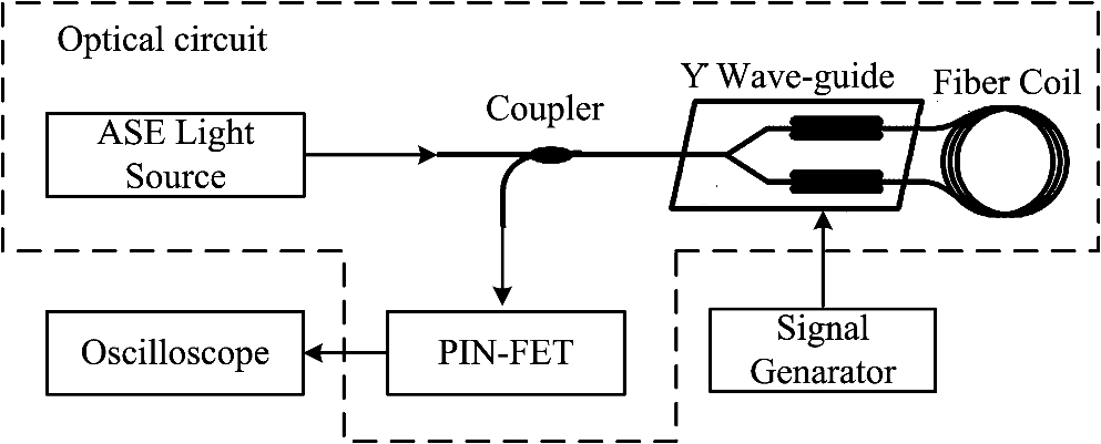
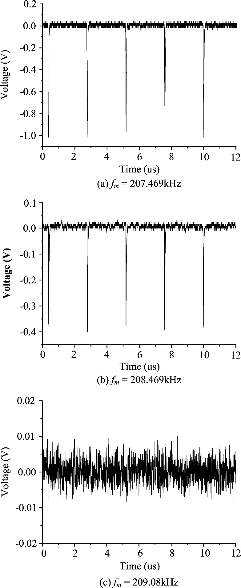
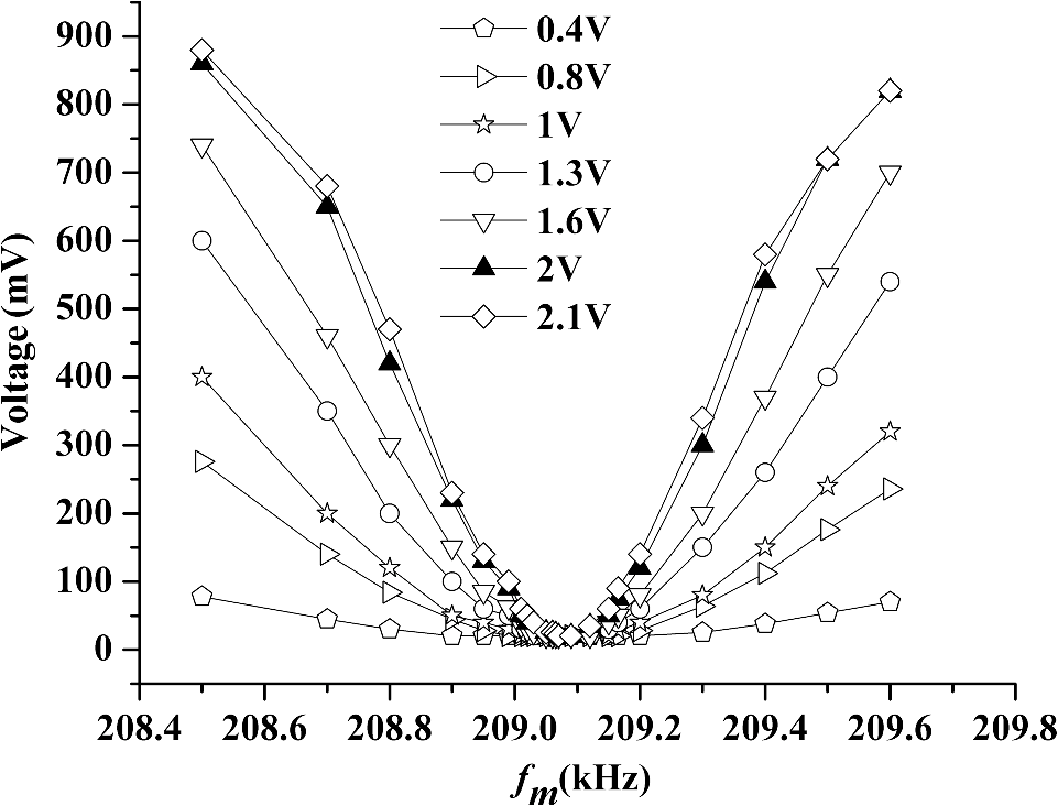
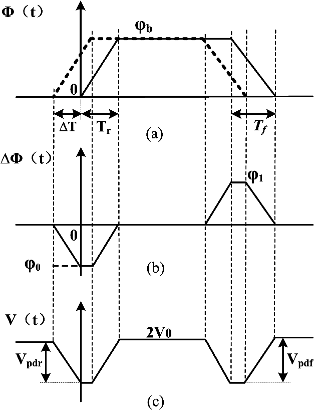
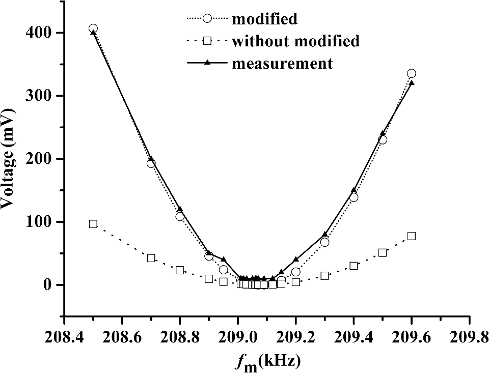
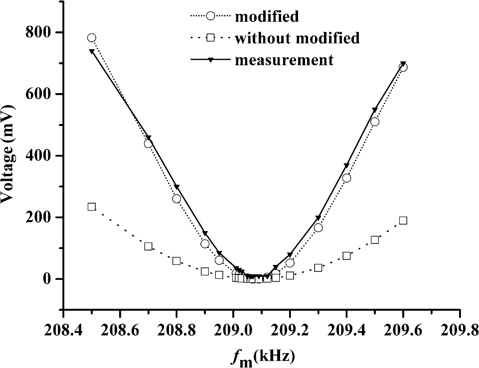
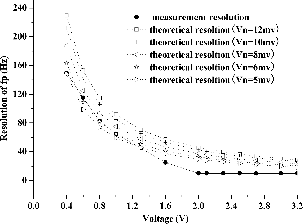
1.

Introduction

Fiber optic gyroscopes (FOGs) are well known as sensors for rotation, which are based on Sagnac effect,¹ and have been under development for a number of years to meet a wide range of performance requirements.^2,3

The eigen frequency is a key parameter of an FOG, as it is essentially defined by the optical path length of the fiber sensing coil. Many sources of rate-output errors are reduced or effectively eliminated by operating the bias modulation at the eigen frequency.^4–7 Establishing an accurate measurement of eigen frequency has been challenging. Existing approaches include the direct measurement methods based on the symmetrical square-wave bias modulation,^8,9 asymmetrical, square-wave bias modulation,^10,11 and techniques based on servo control using an eigen frequency detector.^12–14 The measurement accuracy of former methods was limited by the signal quality of the square-wave, and the latter methods were also limited because of their complexity and cost.

This paper presents a new method for eigen frequency measurement, based on employing the square-wave, over-bias modulation with double eigen frequency. The approach is simple, low-cost, and easy to implement. The Ref. 15 validated the feasibility of the square-wave bias modulation with double eigen frequency primitively, but the obtained performances are not comparable with the present realization in terms of accuracy. In contrast to the approach in Ref. 15, the proposed method makes use of over-bias modulation by adjusting modulation phase depth, and hence, higher accuracy is obtained. In addition, a theoretical model is proposed for describing the relationship between the measurement accuracy and parameters of the bias modulation square-wave.

The paper is organized as follows. Section 2 introduces the measurement principle including the basic idea of the measurement, experimental setup, and experiment results. In Sec. 3, a theoretical model of the method is presented. A comparison between theoretical and experimental results is given in Sec. 4. The last section concludes this paper.

2.

Principle of Measurement

2.1.

Basic Measurement

The method exploits the bias modulation square-wave with double eigen frequency for the phase modulator. Assuming the eigen frequency of a fiber sensing coil is $f_p=1/2\tau$, where $\tau$ is the propagation time of light in the sensing coil, the frequency of the bias modulation square-wave is $f_m=1/T_m$, where the modulated square-wave cycle is $T_m$, duty cycle is 50%, and modulation phase depth is ${\mathrm{\Phi }}_m(t)$. A phase difference between the clockwise (CW) light and counter-clockwise (CCW) light propagating phase in the fiber sensing coil can be expressed as:

Eq. (1)

$$\mathrm{\Delta }{\varphi }_m(t)={\varphi }_m(t)-{\varphi }_m(t-\tau ).$$

According to the Sagnac effect of a FOG, the output of an optical detector $V_{\mathrm{pd}}(t)$ is given by:

Eq. (2)

$$V_{\mathrm{pd}}(t)=V_0\{1+\cos [{\varphi }_s+\mathrm{\Delta }{\varphi }_m(t)]\},$$

where $V_0$ is the voltage generated by the optical detector when phase difference of the two optical beams is 0, and ${\mathrm{\Phi }}_s$ is the phase difference caused by the rotation of the optical fiber around the axis.

2.1.1.

First case: Modulation frequency ${\mathsf{f}}_{\mathsf{m}}<\mathsf{double}\mathsf{e}\mathsf{igen}\mathsf{frequencies}{\mathsf{f}}_{\mathsf{p}}$

When the modulation frequency $f_m$ is less than double eigen frequency $f_p$, the phase and the retardation relations of the two beams of light are shown below in Fig. 1(a)–1(c).

Fig. 1

Phase difference and optical detector’s output when the modulation frequency $f_m$ is less than double eigen frequency 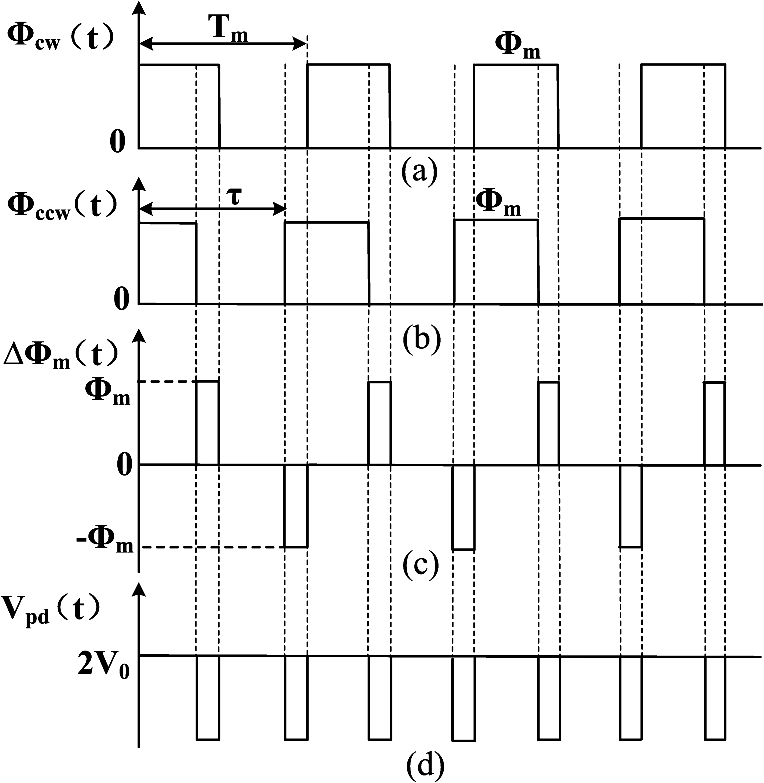$f_p$.

If the optical fiber coil is stationary, ${\mathrm{\Phi }}_s=0$ and the $V_{\mathrm{pd}}(t)$ are obtained as shown in Fig. 1(d); the specific expression is:

Eq. (3)

$$\begin{gathered} V_{\mathrm{pd}}(t)=V_0\{1+\cos [{\varphi }_s+\mathrm{\Delta }{\varphi }_m(t)]\} \\ =\{\begin{array}{ll}2V_0& k{T}_m<t\le k{T}_m-T_m/2+\tau \\ V_0[1+\cos {\varphi }_m]& k{T}_m-T_m/2+\tau <t\le k{T}_m+T_m/2\\ 2V_0& k{T}_m+T_m/2<t\le k{T}_m+\tau \\ V_0[1+\cos {\varphi }_m]& k{T}_m+\tau <t\le (k+1)T_m\end{array}\mathrm{.} \end{gathered}$$

2.1.2.

Second case: modulation frequency ${\mathsf{f}}_{\mathsf{m}}>\mathsf{double}\mathsf{e}\mathsf{igen}\mathsf{frequencies}{\mathsf{f}}_{\mathsf{p}}$

When the $f_m$ is greater than double eigen frequency, the phase and the retardation relations of the two beams of light are shown below in Fig. 2(a)–2(c).

Fig. 2

Phase difference and optical detector’s output when the modulation frequency $f_m$ is greater than double eigen frequency 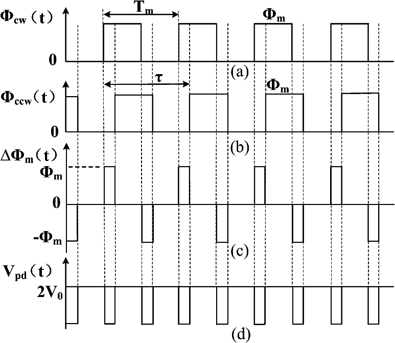$f_p$.

If the optical fiber ring is stationary, ${\mathrm{\Phi }}_s=0$ and the $V_{\mathrm{pd}}(t)$ are obtained as shown in Fig. 2(d); the specific expression is:

Eq. (4)

$$\begin{gathered} V_{\mathrm{pd}}(t)=V_0\{1+\cos [{\varphi }_s+\mathrm{\Delta }{\varphi }_m(t)]\} \\ =\{\begin{array}{ll}{V}_0[1+\cos {\varphi }_m]& k{T}_m<t\le k{T}_m-T_m+\tau \\ 2V_0& k{T}_m-T_m+\tau <t\le k{T}_m+T_m/2\\ V_0[1+\cos {\varphi }_m]& k{T}_m+T_m/2<t\le k{T}_m+\tau \\ 2V_0& k{T}_m+\tau <t\le (k+1)T_m\end{array}\mathrm{.} \end{gathered}$$

2.1.3.

Third case: modulation frequency ${\mathsf{f}}_{\mathsf{m}}=\mathsf{double}\mathsf{e}\mathsf{igen}\mathsf{frequencies}{\mathsf{f}}_{\mathsf{p}}$

When the $f_m$ is equal to double eigen frequency, the phase and the retardation relations of the two beams of light are shown below in Fig. 3(a)–3(c).

Fig. 3

Phase difference and optical detector’s output when the modulation frequency $f_m$ is equal to double eigen frequency 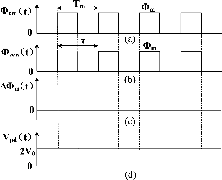$f_p$.

If the optical fiber ring is stationary, ${\mathrm{\Phi }}_s=0$ and the $V_{\mathrm{pd}}(t)$ are obtained as shown in Fig. 3(d); the specific expression is:

Eq. (5)

$$V_{\mathrm{pd}}(t)=V_0\{1+\cos [{\varphi }_s+\mathrm{\Delta }{\varphi }_m(t)]\}=2V_0\mathrm{.}$$

The above analysis shows the output of the optical detector will be a straight line without pulse in theory when the modulation frequency is equal to double eigen frequency. Therefore, the eigen frequency could be directly identified through the observation of optical detector output by oscilloscope.

2.2.

Measurement Setup

The eigen frequency experimental setup is shown in Fig. 4. The optical circuit of the setup is a typical, so-called “minimum configuration,” which provides reciprocal optical paths for two beams counter-propagating in a fiber sensing coil, which is the dotted line in Fig. 4. The optical circuit consists of one light source, a light detector, polarization maintaining (PM) fiber couplers to divide the light into two parts, and one set of ring interferometers to sense orthogonal angular rate.

Fig. 4

Fiber optic gyroscope (FOG) eigen frequency measurement setup.

The advent of low-coherence light sources, such as superluminescent diode (SLD)^4,16–18 and amplified spontaneous emission (ASE) light sources,⁴ permit the elimination of Rayleigh backscattering and Kerr effect errors. An ASE light source is used considering the stable wavelength with temperature sensitivities nearly two orders of magnitude smaller than a SLD. A positive intrinsic negative-field effect transistor (PIN-FET) module is used to convert the light into an electrical signal. The ring interferometer consists of a Y wave-guide (multifunction integrated optic chip, MIOC) and PM fiber coil. The Y wave-guide is a three-port optical gyrochip fabricated at lithium niobate wafer by a high temperature proton exchange technique,¹⁹ and contains a linear polarizer, Y-junction coupler, and two pairs of electro-optic phase modulators. PM fiber is used in order to reduce both the drift caused by the polarization cross coupling and the drift caused by Earth’s outside magnetic field via the Faraday effect.

The light source generates the light which passes through splints evenly into two ways at the Y-junction of the MIOC. The two waves travel inside the fiber-sensing coil in CW and CCW directions, respectively, then interfere back at the Y-junction and arrive at the PIN-FET module. The output of the PIN-FET module is observed by an oscilloscope. At the same time, the bias modulation square-wave is provided by a signal generator.

In the experiment, the length of fiber coil is about 1000 m, the half-wave voltage of the Y waveguide is 3.2 V, the signal generator is the Agilent3320A versatile signal generator, and the oscilloscope is the Tektronix 2024 Digital Oscilloscope.

2.3.

Experimental Results

We can preliminarily determine the eigen frequency of the fiber coil according to the formula $f_p=1/2\tau$ and $\tau =n·l/c$, where $n\approx 1.5$, $l$ represents the length of the fiber coil, and $c$ represents the speed of light in vacuum. According to the parameters of the actual FOG, the transit delay time is about 4.78 μs, and we know the eigen frequency is about 104.6 kHz. So, the modulation frequency of square-wave is about $209\mathrm{kHz}\pm 2\mathrm{kHz}$. The amplitude of the square-wave is 0.8 V (peak-to-peak voltage $V_{\mathrm{pp}}$ is 1.6 V), alternating between $\pi /2$ and $-\pi /2$ in phase, which is a typical amplitude for bias modulation in practice. Then the signal generator generates such a square-wave to modulate the Y waveguide. When changing the frequency and amplitude of the square-wave, the output of the PIN-FET module is simultaneity measured by a digital oscilloscope.

When the modulation frequency changes uniformly from low to high within a few kHz range of eigen frequency, we can clearly observe the process from the oscilloscope, which the changing trends of the pulse amplitude is first high to low, then low to high. The test results are shown in Fig. 5.

Fig. 5

Output signal of the optical detector with different modulation frequencies.

In Fig. 5(a), the frequency of square-wave $f_m$ is 207.469 kHz, which is far from the double eigen frequency, and pulse amplitude is approximately 1.06 V. In Fig. 5(b), $f_m$ was 208.469 kHz, which is not so far away from the double eigen frequency, and pulse amplitude is approximately 436 mV. In Fig. 5(c), $f_m$ was 209.08 kHz, which is very close to the double eigen frequency, and the detector output is approximated to a straight line. From Fig. 5, it is obvious the pulse amplitude of detector’s output decreases while reducing the difference between $f_m$ and the double eigen frequency, and the detector’s output is approximated to a straight line when the two are very close.

In our experiment, we also observe the phenomena of modulation dead area described in Ref. 11. When the observation range is zoomed out to 0.5 kHz or so, and modulation frequency increased from low to high, the pulse amplitude first went from high to low, then low to high in some frequency ranges. In these frequency ranges, it is difficult to distinguish between the pulse and noise because the pulse drowns in the noise, and the increasing process from low to high is again observed only across the frequency range.

The existence of a modulation dead area limits the accuracy of the eigen frequency measurement. To solve the problem, a popular method is to shorten the rise and fall time of a square-wave. In this study, a more simple and effective way is presented, which uses square-wave, over-bias modulation to improve the measurement accuracy by increasing the modulation phase depth. We proved the modulation phase depth can affect accuracy of the eigen frequency measurement, and the experiment results are shown in Figs. 6 and 7.

Fig. 6

Amplitude of the optical detector’s output under different modulation voltages.

Fig. 7

The relationship between amplitude of the modulation square-wave and measurement resolution of eigen frequency.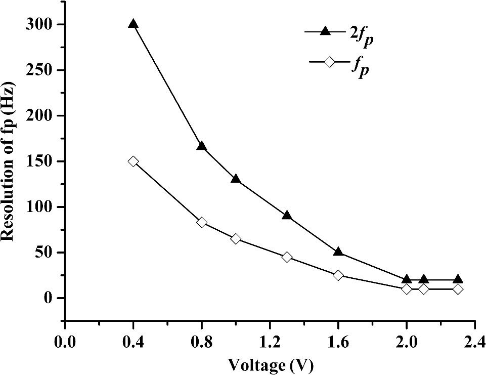

Figure 6 illustrates how the amplitude of the pulse changes with different modulation phase depths by verifying modulation voltages; the $x$-axis represents the modulation frequency, and the $y$-axis indicates the amplitude of the detector’s output pulse. As shown in Fig. 6, we can effectively reduce the range of the modulation dead area by increasing modulation voltage. The minimum modulation dead area is obtained when the amplitude of the square-wave is 2 V (the modulation phase depth about $5\pi /4$), so the measurement resolution of eigen frequency can reach 10 Hz, which already satisfies most FOGs. If the modulation voltage increases continually, the range of the modulation dead area will no longer change. From the results, we know the eigen frequency of this FOG is between 104.535 and 104.545 kHz. According to the symmetry of the curves in Fig. 6, the eigen frequency is 104.54 kHz, and the measurement accuracy is $\pm 5\mathrm{Hz}$.

Figure 7 shows a curve of the relationship between the amplitude of the bias modulation square-wave and the accuracy of eigen frequency measurement; the $y$-axis represents the measurement accuracy, and the $x$-axis represents the amplitude of the square-wave. In Fig. 7, the upper line represents the measurement of the double eigen frequency; the lower line represents the measurement of the eigen frequency. We find that the minimum eigen frequency resolution can be improved from 150 to 10 Hz when the amplitude of the square-wave is increased from 0.4 to 2 V (the modulation phase depth from $\pi /4$ to $5\pi /4$), but the measurement accuracy does not change when the amplitude of the square-wave increases from 2 V.

3.

Theoretical Model

The modulation waveform generated by the actual circuits is not the ideal square-wave, in which the output characteristics are affected by the geometric length of the fiber, the refractive index, and performance of electronic components of the signal processing system. In addition, distributed capacitances inside the Y waveguide, the matching degree of the load impedance, and signal processing circuit have effects on the waveform as well. Thus, we assume the actual square-wave is a trapezoidal wave, where amplitude is $V_m$, corresponding modulation phase depth is ${\varphi }_b$, rise time is $T_r$, and falling edge time is $T_f$.

The phase relationship between the CW light and CCW light within one period is shown in Fig. 8(a), when the modulation frequency $f_m$ is less than the double eigen frequency $f_p$. Wherein, $\mathrm{\Delta }T=\mathrm{\Delta }f/2f_m{f}_p$ represents the time delay on the transmission of the two light beams, $\mathrm{\Delta }f$ is the difference between $f_m$ and 2$f_p$. The phase deference between the CW light and CCW light is shown in Fig. 8(b), where

Fig. 8

Schematic of theoretical model.

Considering the difference of the square-wave in the model and the actual waveform, correction coefficient $\alpha$ of the rising edge and correction coefficient $\beta$ of the falling edge are brought in our model. Then the two formulas above become:

Because of the cosine curve relationship between the detector’s output and the Sagnac phase shift, the detector’s output pulse amplitude $V_{\mathrm{pdr}}$ at rising edge and $V_{\mathrm{pdf}}$ at falling edge can be gained, respectively, which is shown in Fig. 8(c):

In a similar way, when the modulation frequency $f_m$ is greater than the double eigen frequency $f_p$, we can also obtain Eqs. (12) and (13):

Equations (10)–(13) show that since the detector output is an even function, the equations are similarly obtained from both cases ($f_m<2f_p$ or $f_m>2f_p$). Thus, Eqs. (12) and (13) can characterize our measurement method. According to Eqs. (12) and (13), we can analyze the influence of various parameters on the measurement accuracy.

4.

Discussion: Comparison between Theory and Experiment

For the convenience of calculation, we assume the rise time $T_r$ is equal to the fall time $T_f$, as are the rising correction factor $\alpha$ and the falling correction $\beta$ factor, according to the parameters of practical square-wave. In the theoretical model, the parameters are summarized as follows: $T_r=T_f=40\mathrm{ns}$, $f_p=104.54\mathrm{kHz}$, $\alpha =\beta$.

Figure 9 shows the comparison of theoretical and experimental results at $V_m=1\mathrm{V}$ ($V_{\mathrm{pp}}=2\mathrm{V}$), where the $x$-and $y$-axes represent modulation frequency and detector output pulse amplitude, respectively. Then, in Fig. 9, the calculations include the uncorrected situation ($\alpha =\beta =1$), represented by the lower dotted line, and corrected situation ($\alpha =\beta =2.2$), represented by upper dotted line. As shown in Fig. 9, a great deviation between uncorrected results and practical results, represented by the solid line, takes place, especially when modulation frequency is far away from the eigen frequency. However, the corrected results agree with experimental results.

Fig. 9

Theoretical and experimental results at $V_m=1\mathrm{V}$.

Figure 10 shows the comparison of theoretical and experimental results at $V_m=1.6\mathrm{V}$ ($V_{\mathrm{pp}}=3.2\mathrm{V}$). Similarly to Fig. 9, the corrected results agree with experimental results. From Figs. 9 and 10, we can see that the correction model can better describe the actual measurement conditions.

Fig. 10

Theoretical and experimental results at $V_m=1.6\mathrm{V}$.

And then, we can use Eqs. (12) or (13) from the theoretical model to analyze the effects on the measurement caused by the square-wave modulation voltage and the reasons why modulation dead area exists.

According to the theoretical model, we can obtain a very high measurement resolution of eigen frequency; however, because of output background noise generated in the test system, it needs a pulse amplitude value greater than background noise in order to measure the existing pulse effectively. Otherwise, it is difficult to identify whether it is noise signal or pulse signal.

Assuming the noise signal is $V_n$, we can obtain from Eqs. (12) or (13):

From Eq. (15), we know the minimum frequency difference $\mathrm{\Delta }f$ or the modulation dead area is affected by factors such as noise signal $V_n$, modulation phase depth ${\varphi }_b$, rise time $T_r$, or the fall time $T_f$. Similarly to methods in Refs. 89.10.–11, an effective way to improve the detection accuracy is by reducing $T_r$ or $T_f$. For a fixed $T_r$ or $T_f$, increasing square-wave amplitude leads to adding modulation phase depth, which can also reduce modulation dead area and detect smaller frequency difference $\mathrm{\Delta }f$, thereby improving the detection accuracy of eigen frequency. Compared with the method of reducing rise and fall times, it is easier and simpler to increase the modulation phase depth ${\varphi }_b$ by changing the square-wave voltage amplitude. So, adjusting the modulation phase depth is a better choice in practice.

We carried out numerical calculations with respect to ${\varphi }_b$ and the results are shown in Fig. 11. In Fig. 11, the dotted lines represent the theoretical resolution of eigen frequency under various noise signals ($V_n$), and the solid line represents the measurement resolution of eigen frequency. The graphs in Fig. 11 illustrate that the theoretical resolution of eigen frequency is inversely proportional to ${\varphi }_b$ if noise signal $V_n$ is a fixed value. In addition, the theoretical resolution of eigen frequency can be improved with the decrease of $V_n$.

Fig. 11

Comparison of theoretical and experimental measurement resolution of eigen frequency.

Figure 11 also shows the experimental values are mainly consistent with the theoretical values. This variance is due to the fact that the actual square-wave is not a perfect wave, its rising edge and falling edge change nonlinearly, but the theoretical model takes the square-wave as a trapezoidal wave. In addition, because of the characteristic of an inversely proportional function, there is always a section of small curvature curve for the function $\mathrm{\Delta }f$ (${\phi }_b$). In this section, the detected frequency difference $\mathrm{\Delta }f$ changes slightly, even with a large modulation phase depth. Furthermore, the background noise is 5 mV or so, and not a fixed value in actual condition, so it is difficult to identify whether the frequency is noise signal or pulse signal in the section. Therefore, the measurement accuracy does not change when the amplitude of the square-wave increases above 2 V.

The experiment demonstrates very good accuracy compared to the other direct measurement methods (the resolution declared in Ref. 10 is 100 Hz, and the resolution declared in Ref. 15 is 75 Hz), with advantages of simple, low-cost, and easy to implement. The accuracy of the proposed method is better than $\pm 5\mathrm{Hz}$ under suitable modulation phase depth, which can accommodate the eigen frequency measurement of most FOGs, such as inertial navigation grade FOGs with 0.01 deg per hour bias stability performance, and under inertial navigation grade FOGs.

To further improve the measurement accuracy, further reduction of the noise, optimizing the power supply and signal source, reducing the square-wave signal rise and fall times, and using some appropriate filtering approaches, and so on, should be carefully considered.

5.

Conclusion

We propose a new measurement method based on square-wave, over-bias modulation with double eigen frequency. The proposed method was investigated both theoretically and experimentally. A theoretical model of the method is also presented. Experimental and theoretical results are shown to be consistent. Comparing to the existing methods, this approach has advantages of simple, low-cost, and easy to implement. It can greatly improve the accuracy of the eigen frequency measurement without needing additional hardware in the existing gyro system. The accuracy of the eigen frequency measurement is better than $\pm 5\mathrm{Hz}$ under suitable modulation phase depth, which can accommodate the eigen frequency measurement of most FOGs.