|
|
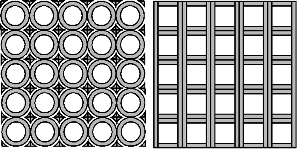
1.IntroductionThis article discusses methods for phase sensitive x-ray characterization in inertial confinement fusion. Fusion is the process that powers stars, and numerous efforts are under way to achieve laboratory demonstrations of breakeven, more energy released via the fusion process than input to initiate the fusion reaction. In man-made fusion, two light nuclei are brought together at sufficiently high density and for a sufficiently long time to overcome the Coulomb force between the two nuclei such that their respective nuclei are fused together. That process liberates more energy than is required to fuse the two nuclei together and hence is being pursued as an energy source. In man-made fusion, the two nuclei are generally deuterium and tritium due to the smaller coulomb barrier that must be overcome and the higher reaction rate at lower temperature than other possible reaction rates. In inertial confinement fusion the deuterium-tritium (DT) fuel is compressed to very high densities for a relatively short time. This compression is driven directly or indirectly by absorption of radiation, optical, x-ray, or ion, in a fuel capsule. This fuel capsule is composed of an outer ablator and an inner region containing deuterium and tritium. The radiation is absorbed by the ablator whose mass is ablated by the absorbed energy driving shock waves, which then compress the deuterium-tritium to high density and temperature where the deuterium/tritium ions can fuse together. This fusion process produces a neutron and an alpha particle and releases more energy than is required to force the deuterium/tritium nuclei together. To understand the fusion process it is necessary to fully characterize the fuel capsule both before and during the implosion process. Due to the high densities and small spatial scales present in the fuel capsule this characterization must be done with x-rays or with high-energy electrons or ions. To detect the light deuterium and tritium atoms in the fuel capsule, relative to the ablator composed of carbon, hydrogen, and higher atomic number dopants such as silicon, techniques such as phase contrast x-ray imaging are employed. Phase contrast imaging can readily detect boundaries, such as the position of the DT ice layer, but it is difficult to achieve quantitative information with regard to the phase shift. The image contrast is optimized on the detector at different relative distances depending on the phase gradients in the object. In the implosion phase of the fuel capsule, to date, only absorption radiography has been employed , however, some radiographs have shown evidence of refraction enhanced features.1 It is desirable, however, to recover both the absorption and the phase shift of the x-rays passing through the object. In so doing, more information is available to assess, for instance, the mixing of the higher atomic number ablator material with the lower atomic number fuel. Developing x-ray phase sensitive imaging techniques, which are more quantitative than phase contrast imaging and can be obtained with a single image, for the imploding fusion capsule is highly desirable. A number of wavefront sensing techniques have been proposed and some implemented in the x-ray regime to measure either the phase, the gradient of the phase, or the Laplacian of the phase. The first hard x-ray interferometer, implemented on a synchrotron source, used three partially transmitting Bragg crystals and was manufactured from a highly pure single silicon crystal to minimize vibrational effects.2 Interferometers implemented in the soft x-ray regime have utilized gratings3 and mulitlayer mirrors4 to realize Michaelson and Mach-Zehnder designs. Generally interferometric techniques require very stable platforms and higher spatial coherence than obtainable with point projection x-ray backlighters and microfocus x-ray tubes. Phase retrieval techniques have been proposed5 to determine the phase of an x-ray probe beam and implemented6 to control an x-ray adaptive optic in a synchrotron beamline; however, these techniques benefit from measurements made at multiple distances from the object. Numerous techniques have been used to determine the gradient in the phase, which can be more robust against vibrations. Various Hartmann sensors have been proposed and implemented on soft x-ray lasers ranging from an array of holes,7,8 zone plates,7 multilayer mirrors,9 and refractive lenses.10 One-dimensional shear interferometers based on Lloyd’s mirror have been demonstrated,11 and several instruments based on the principles of Moire’ deflectometery have been realized with soft x-ray lasers, both with shears in only one dimension12 and in two dimensions.13 These latter instruments are less susceptible to vibrations than the phase-measuring interferometers or the one-dimensional shear interferometer based on a Lloyd’s mirror but require careful separation distance and angular rotation of the gratings, which still make these latter instruments susceptible to vibrations. Two-dimensional shearing interferometers,14,15 based on two orthogonal phase gratings in the same plane, have also been proposed to measure the wavefront of an x-ray beam. These two dimensional shearing interferometers14,15 place the periodic structure in a single plane and are therefore expected to be much less susceptible to vibrations and alignment errors and are expected to be more achromatic than the two dimensional Moire’ deflectometers. Curvature sensors, which measure the Laplacian of the phase, could also be implemented in the x-ray regime,16 and phase contrast imaging1 itself measures the Laplacian of the phase. Again, the techniques that measure the Laplacian of the phase generally require measurements in multiple planes to quantitatively measure the phase and hence are more difficult to implement on a single shot in the hard x-ray regime. In this article, phase reconstructions from a two-dimensional shearing interferometer, based on two orthogonal phase gratings in a single plane, and a Hartmann sensor are compared. Both of these sensors can measure the two-dimensional wavefront gradient of an x-ray beam, as well as the x-ray absorption. These instruments measure the two-dimensional wavefront gradient in a single measurement and do not require multiple measurements or movement of the grating, making them suitable for measuring the implosion of fusion capsules. The two-dimensional grating or array of holes, in the case of the Hartmann sensor, can be made on a single membrane or cut from a single thin film, making it insensitive to both vibrations and alignment. A two-dimensional shearing interferometer based on crossed phase gratings has been implemented previously in the visible regime.17 In this case the crossed phase gratings were formed by etching a chess board pattern into glass. Hartmann sensors have also been implemented in the visible regime.18 1.1.Two-Dimensional Shearing InterferometerThe shearing interferometer uses orthogonal phase gratings, which can be designed as either two crossed phase gratings or a single checkerboard pattern as it’s two-dimensional wavefront sensor, as shown in Fig. 1. The phase gratings are designed such that the even orders of the grating are eliminated. In order for the efficiency of the even orders, greater than the order, of a transmission grating to go to zero at x-ray wavelengths, the width of the slits must be half of the grating pitch.8,9 In addition, for the efficiency of the order of the grating to go to zero, there must be negligible absorption and the bar structure of the grating must produce a shift of radians relative to the slits of the grating. The coherency requirements for the two-dimensional x-ray shearing interferometer are such that the source is required to be nearly spatially coherent. This is consistent with using a spatially filtered x-ray source. The requirements are such that the pinhole in front of the x-ray source be sufficiently small so that the diffractive spreading of the x-rays exceed the pitch of the gratings or , where L is the distance between the source and the grating, is the wavelength, is the diameter of the x-ray source and is the pitch of the grating. For a grating pitch of , an x-ray wavelength of angstrom and a separation of between the x-ray source and the crossed phase grating, the requirements on the pinhole size are that it be less than in size. Extended x-ray sources can also be used when the source is appropriately made periodic. By placing a Ronchi ruling or grating in front of the extended source, it can be made to appear as a spatially coherent source as photons from the different regions of the source can be made to align the peaks of the diffraction pattern in the same location on the detector thereby forming good contrast fringes.19 This has the advantage of greatly increasing the amount of x-rays impinging on the sample but the disadvantage of convolving the measurement with the nearest neighbors, which will affect the high spatial frequency information. 1.2.Hartmann SensorsThere are several potential implementations for an x-ray Hartmann sensor. This can be simply an array of holes,7,8 zone plates,7 multilayer mirrors,9 or refractive lenses.10 The Hartmann wavefront sensor based on an array of holes is shown schematically in Fig. 2. The displacement of the spots on the detector is proportional to the wavefront gradient across the corresponding hole in the Hartmann mask. This approach uses an amplitude mask, which throws the majority of the signal away. In the visible regime all of the signal is used by modifying the Hartmann mask to utilize a lenslet array. In the x-ray regime this signal loss can be avoided using an array of phase zone plates as shown in Fig. 3. This can be accomplished using either circular or two crossed one-dimensional zone plates. In either case, the x-ray spot on the detector must be larger than a pixel size such that a very poor resolution zone plate would be required. Assuming a subaperture size of 20 μm, a charge coupled device (CCD) pixel size of 5 μm and two zones, inner zone has radius of 7.07 μm and outer zone has a radius of 10 μm. The focal length at 0.8 keV (8 keV) would be 0.032 m (0.32 m) and the spot size on the camera would be . Fig. 2Hartmann wavefront sensor implemented with an array of holes. The displacement of the spots on the detector is proportional to the wavefront gradient across the corresponding hole in the Hartmann mask.  The requirements placed on the transverse spatial coherence for a Hartmann sensor are not as stringent as for the shearing interferometer. In its simplest implementation, the Hartmann screen would consist of a regular array of holes with the displacement of the x-rays traveling through the holes providing the phase gradient information and the amplitude of the x-rays providing the absorption information. The sensitivity expected from a Hartmann sensor can be calculated analytically as where is the angular extent of the source, is the wavelength of the source, is the size of the subaperture, is the source spot size, is the distance between the source and the Hartmann sensor and SNR is the signal-to-noise-ratio of the measurement.20 For an x-ray spot size of 20 μm, a distance between the x-ray source and the Hartmann screen of 40 cm and an SNR of 20, one would expect to measure angular deflections of . The Hartmann wavefront sensor is therefore degraded by a larger x-ray spot size but to a lesser extent than the two-dimensional shearing interferometer.2.Phase ReconstructionThe experimental geometry that is simulated in this article is shown explicitly in Fig. 4 for both the shearing interferometer and the Hartmann wavefront sensor. The object is placed in a diverging x-ray beam, which is, in turn, magnified onto the wavefront sensor and onto the CCD detector. This allows both the phase and the absorption information to be recovered. Fig. 4Experimental geometry, with either a two-dimensional crossed phase grating or a Hartmann amplitude mask, which would be used to measure the object’s phase and absorption. 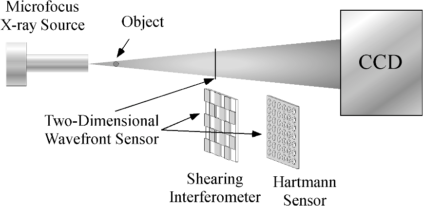 By placing the object in an expanding beam, there is a large focus term on the phase. There are at least two approaches to recovering the phase in the presence of a large focus term. The first is to use an iterative technique14,21 to reconstruct the large phase. A second approach is to perform the phase reconstruction in collimated space, which is the technique that will be used in this article.15 This latter technique is effectively used for curvature wavefront sensor simulations.11,12 The simulation geometry is then shown in Fig. 5. The far right-hand side shows the geometry of the experiment in which a micro-focus x-ray source would reside in the location of the focus of the lens and illuminate the object and x-ray mask with a spherically diverging beam, which would then be collected with the x-ray CCD camera. Each of these devices, the x-ray source, the object, the x-ray mask and the x-ray CCD camera, has an object plane in collimated space on the left-hand side of the lens as shown in Fig. 5. Thus the simulation can be performed in collimated space with the appropriate magnification placed on each of the objects. Fig. 5Simulation geometry used to calculate the phase of an object for either the two-dimensional shearing interferometer or the Hartmann sensor by performing Fresnel propagation in collimated space. 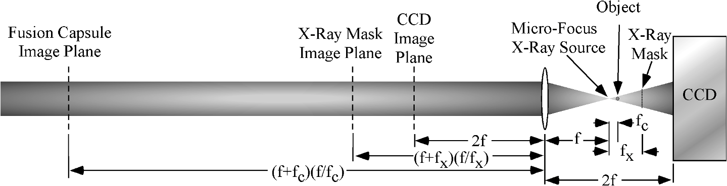 2.1.Characterization of a Stationary Deuterium-Tritium Fusion Capsule Phase ProfileThe experimental measurement setup for the characterization of the fusion capsules consists primarily of a micro-focus x-ray source, the fusion capsule itself, a phase flattener, the wavefront sensor, a filter, and the detector as shown in Fig. 4. The micro-focus x-ray source will be assumed to contain a source size of approximately 5 μm in diameter. Current experimental work with phase contrast imaging uses a micro-focus x-ray source which has a source size of 5 μm in diameter and a tungsten anode operating at 50 kV.22 The L shell emission is in the 8 to 11 keV x-ray range. Operating the source at 50 kV will result in significant bremsstrahlung radiation at higher x-ray energies.23,24 The detector, however, is an x-ray CCD camera, which becomes optically thin to the higher-energy photons.22 The lower-energy x-rays can be removed and a narrower energy range within the L-shell emission can be selected by filtering with a thin foil such as copper. The fusion capsules are spherical in shape and consist of an outer ablator shell with an inner layer of DT fuel. The fusion capsules have an overall diameter of approximately 2 mm. In the case of an outer CH ablator, the thickness of the ablator shell is approximately 190 μm and the DT layer on the inside of the capsule is approximately 68 μm thick. At x-ray wavelengths the index of refraction is expressed as , where gives rise to a phase shift as the x-rays pass through the sample and the term results in absorption. The length for a phase shift, , is expressed as and the absorption length, , is written as . At an x-ray energy of 10 keV, the x-rays have a wavelength of . The phase shift due to the CH ablator, , at this wavelength is , , or a phase shift over a distance of 25 μm. The phase shift due to the DT, , at this wavelength is , , or a phase shift over a distance of 150 μm. The CH represents a line-integrated depth of or 47.8 radians and the DT represents a line-integrated depth of 136 μm or 2.8 radians. The contribution from both sides of the CH ablator and from both DT ice layers yields a combined phase shift of . The DT ice layer in the fusion capsule forms grain boundaries, which range between 1 to 10 μm in depth. Based on experimental data, it is believed that the maximum grain boundary depth that can be tolerated on a fusion shot is without unacceptably impacting the yield. In addition the maximum cross-sectional area for a given grain boundary that can be tolerated is . It is therefore desired to reject all targets that have grain boundary depths that exceed the 5 μm depth and that have a cross-sectional area greater than . A quantitative method is therefore needed to measure the phase profile of a given capsule to determine if any of the grain boundaries present in the DT layer exceed these parameters. A 5 μm depth at the grain boundary in the DT ice layer would then make a difference in the phase of 5 μm out of the line-integrated DT depth of 130 μm. This is in addition to an RMS surface roughness for the DT ice layer. That represents only a 3.8% difference in the path length or 0.098 rad in the phase shift for the crevice, and 0.4% or 0.0098 rad RMS due to the surface roughness. The wavefront sensors therefore must be able to detect the gradients from a phase shift of only representing the peak of the ice grain boundary against the background phase, which would be approximately 50.6 radians in the center, to greater than double that at the edge of the capsule 1 mm away. For this article, an analytical model for the grain boundary is assumed. The phase contribution due to the grain boundary, , is represented in analytical form by the expression , where is the peak amplitude of the phase from the grain boundary and is the spatial coordinate in μm. The analytic phase gradient is expressed as for x greater than 0. Based on these analytic expressions, the refraction angle, , of x-rays passing through the ice grain boundary can be approximated as for greater than 0. A phase flattener is proposed to reduce the low-order phase response from the capsule geometry. The phase of the fusion capsule itself will vary from approximately 50 radians in the center to more than double that at the edge of the capsule a millimeter away. This is not critical as the measurement will primarily concentrate on the central region of the fusion capsule with two additional orthogonal views to provide information on grain boundaries over the entire capsule. With this phase flattener in, however, the difference between the reference spot locations measured before the fusion capsule and flattener are inserted and the spot locations measured after the fusion capsule and flattener are inserted will provide a direct measurement of the rms surface roughness and the depth and cross-sectional area of the grain boundaries. The phase flattener would then represent an inverse phase to the fusion capsule and could be placed immediately before or after the fusion capsule. For the simulations, the following assumptions are made; 5.4 μm CCD pixel pitch, 43.2 μm x-ray grating pitch (in collimated space), , and , where , , and are the fusion capsule plane, the x-ray mask plane and the focal length of the “lens,” respectively. In an actual experiment the gratings would have a pitch of in the spherically expanding x-ray beam and the x-ray CCD would have pixel size. Given these assumptions, the fusion capsule is magnified by a factor of 3.67 onto the x-ray mask and a factor of 11 onto the x-ray CCD camera. The capsule is 2.2 mm in diameter, which would require a CCD with an active area of at least 2.4 cm. This is consistent with 4096 pixels at . The x-ray CCD will measure the wavefront gradient at a scale of 4 μm on the capsule (43.2 μm in collimated space). The simulations are performed on one-quarter of the fusion capsule, , such that across the simulation box there are 2048 pixels on the x-ray CCD. Each grating feature with 21.6 μm pitch spacing represents an area on the x-ray CCD of CCD pixels or a total of 512 simulation pixels. The simulations are performed with both read noise and Poisson noise. For the simulations shown the read noise was assumed to be 2 e-RMS, and the x-rays were assumed to produce several hundred thousand photoelectrons per every CCD pixel. The simulations begin by defining a uniform field at the image plane of the fusion capsule located at the left-hand side of Fig. 5 and assuming a point x-ray source. The simulations were performed with simulation pixels covering a range on the camera of per simulation pixel, representing . on the fusion capsule itself. One quarter of the fusion capsule sphere was simulated with an initial phase profile of 0.026 rad RMS, RMS, placed on the fusion capsule to simulate surface roughness. A Kolmogorov turbulence profile was assumed for the surface roughness of the DT ice layer. In addition to the phase profile representing the surface roughness of the DT ice, six DT ice grain boundaries were placed across the fusion capsule with each one having a width of 50 μm (500 μm in collimated space) but different lengths, depths and angles, as shown in Fig. 7(a). In particular, a long horizontal and vertical ice grain boundary were introduced, which had a 5 μm depth. The phase representing the fusion capsule and phase flattener were then used to construct a new field, which was then Fresnel propagated to the two-dimensional x-ray transmission grating shown in Fig. 6(a). The periodic phase pattern representing the crossed phase grating is then added to the field, and the field is propagated to the x-ray CCD camera. When a periodic structure is placed in a beam, images of that structure will appear downstream of the object as discovered by Talbot.25 More precisely, if a phase grating is placed in the beam composed of alternating equal width bars of 0 and phases, then the field at the location of the phase structure will be reproduced a distance downstream of the phase structure. In this expression, is the Talbot distance, d represents the pitch of the phase grating and is the wavelength of the source. At distances of and , the initial phase pattern across the beam has become uniform and the initially uniform intensity has acquired the periodic structure of the initial phase pattern with the pitch of the intensity pattern equal to half that of the original phase grating. At a distance of , the phase pattern is reversed from the original phase grating, and the intensity pattern is uniform such that this particular location cannot be used for wavefront sensing. Fig. 6The phase mask used for the shear interferometer (a) results in the spatial profile of the x-rays impinging on the simulated detector (b). The amplitude mask used for the Hartmann sensor (c) produces the spatial profile of the x-rays impinging on the simulated detector (d). 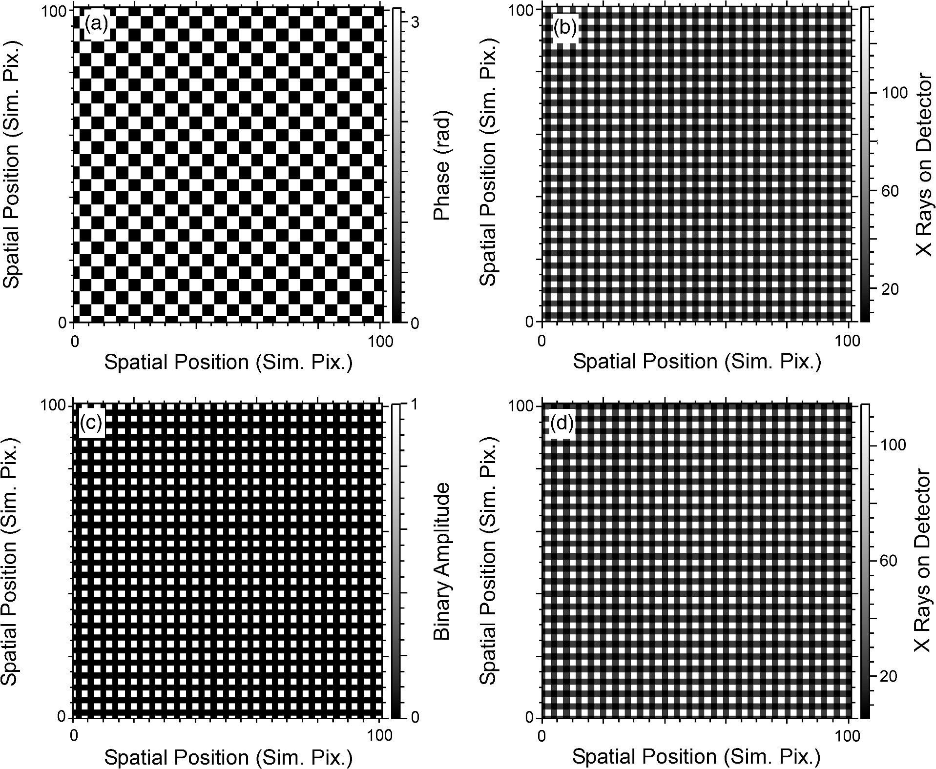 Fig. 7The applied phase pattern representing the fuel capsule (a) the reconstructed phase pattern from the shear interferometer (b) and the reconstructed phase pattern for the Hartmann mask (c). 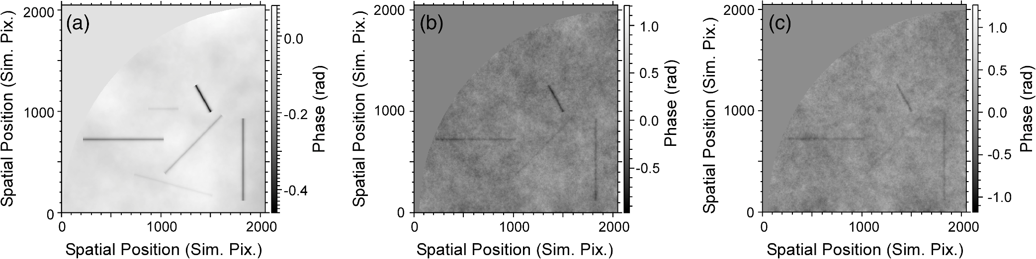 The x-ray masks for the shearing interferometer are shown in Fig. 6(a) and 6(c), respectively. The respective two-dimensional array of spots from the masks are then shown in Fig. 6(b) and 6(d) for the shearing interferometer and the Hartmann mask, respectively. A comparison between these images shows how similar these wavefront sensors are from the perspective of analyzing the phase and amplitude of the object. In Fig. 6(b) and 6(d), the images represent the number of x-rays impinging upon the detector and not the number of photoelectrons generated in the detector. The two-dimensional reconstructed phase from the shearing interferometer and the Hartmann sensor is displayed in Fig. 7 along with the phase profile imparted on the object for the simulation. In particular, the applied phase is shown in Fig. 7(a), the reconstructed phase from the shearing interferometer in Fig. 7(b), and the reconstructed phase from the Hartmann sensor in Fig. 7(c). For both the shearing interferometer and the Hartmann sensor the four largest phase amplitudes resulting from the grain boundaries in the DT layer are visible in the reconstruction, but the two smallest phase amplitude DT ice grain boundaries are not obviously identifiable. Figure 8 shows a comparison between the reconstructed spatial phase and the applied spatial phase across a DT ice grain boundary. This spatial profile is averaged along the length of the DT ice grain boundary and will be referred to as a line out across the ice grain boundary. Specifically, Fig. 8(a) shows line outs across two of the reconstructed DT ice grain boundaries, averaged along the length of the grain boundary for the shearing interferometer. The solid black line represents the analytic phase profile applied to the vertical and horizontal ice grain boundaries in Fig. 7(a). The light gray dashed line represents the reconstruction of the long horizontal DT ice grain boundary seen in Fig. 7(a), and the dark gray dashed line represents the reconstruction of the vertical DT ice grain boundary seen in Fig. 7(a). Figure 8(b) shows line outs across two of the reconstructed DT ice grain boundaries, averaged along the length of the grain boundary for the Hartmann sensor. The solid black line represents the analytic phase profile applied to the vertical and horizontal ice grain boundaries in Fig. 7(a). The light gray dashed line represents the reconstruction of the long horizontal DT ice grain boundary seen in Fig. 7(a), and the dark gray dashed line represents the reconstruction of the vertical DT ice grain boundary seen in Fig. 7(a). Fig. 8Line outs of the applied phase (solid black line) compared with the reconstructed phases from the main horizontal DT ice grain boundary in Fig. 7(a) (dashed light gray) and the main vertical DT ice grain boundary in Fig. 7(a) (dashed dark gray) for the shearing interferometer (a) and the Hartmann mask (b). 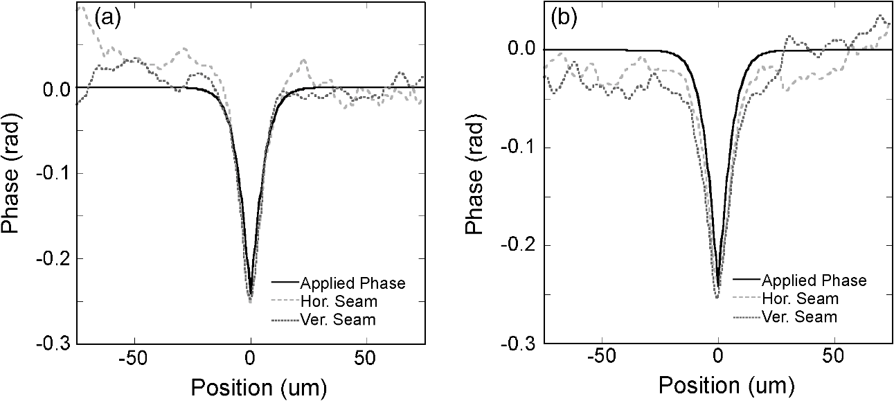 2.2.Characterization of an Imploding Deuterium-Tritium Fusion Capsule: Detection of High-Frequency Spikes of Ablator Material Seen in DT Fuel Capsule ImplosionsThis section compares the phase reconstruction of a shearing interferometer and Hartmann sensor for an imploding DT fusion capsule. This is modeled with an “asterisk” phase profile to test the ability of these wavefront sensors to detect spikes of ablator material seen in DT fuel capsule implosions.26,27 In both simulations, x-rays were assumed to be diverging from a point projection x-ray source, a laser-driven x-ray backlighter, with an f/# of 110, where the f/# is defined as the focal length of the focusing optic divided by the diameter of the x-ray beam. The simulations were performed with 10 keV x-rays, and the geometry of the simulation is shown in Fig. 4. The object was placed 0.1 m from the point projection x-ray source and the mask, phase or amplitude was placed 0.367 m from the focus with the detector placed 1.1 m from the focus. As a consequence the object was magnified a factor of 3.67 onto the mask, and the mask was, in turn, magnified a factor of three onto the detector. The phase gratings for the shearing interferometer were simulated with bar and trough widths equal to four simulation pixels or 21.6 μm. In the case of the Hartmann sensor, the amplitude Hartmann mask was also simulated with the pitch of the holes equal to four simulation pixels or 21.6 μm. As in the previous section, the simulations utilized wave optics to transport the electric field between the various planes containing phase or amplitude objects. The grating structure or Hartmann mask and the phase object are added to the electric field after the field has been propagated to their respective locations. The wavefront is reconstructed from the simulated spots by first locating the displacement of each of the spots with a center-of-mass centroider28 and then reconstructing the resulting gradients with a multigrid wavefront reconstructor.29 Figure 9(a) and 9(b) represents the intensity pattern at the detector with an “asterisk-shaped” phase object in the beam. Based on the spot patterns in Fig. 9(a) and 9(b), the local gradients were determined, the phase reconstructed, and the amplitude solved for. The two phases were then reconstructed using a multigrid algorithm26 to determine the phase of the object. The results of this phase recovery process are shown in Fig. 10(b) and 10(c) for the shearing interferometer and the Hartmann sensor, respectively, with the applied phase being displayed in Fig. 10(a). Fig. 9Intensity profiles at the detector for both the two-dimensional shearing interferometer (a) and the Hartmann sensor (b). The size of the simulation box shown, 200 pixels, represents 1.08 mm in collimated space and 98 μm at the capsule plane. 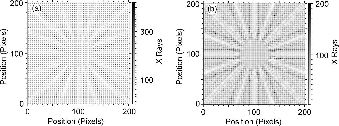 Fig. 10Retrieved phase object with the two-dimensional shearing interferometer and the Hartmann sensor; the actual phase of the object placed in the expanding x-ray beam (a) the reconstructed phase for the shearing interferometer (b), and the reconstructed phase for the Hartmann sensor (c). The outer diameter of the “asterisk” pattern/spikes, 1000 pixels, represents 5.4 mm in collimated space and 490 μm at the capsule plane. 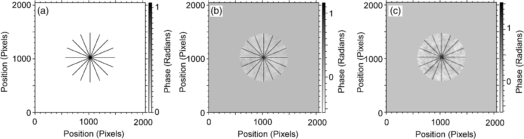 3.DiscussionIn the case of characterization of a stationary DT fusion capsule phase profile in Sec. 2.1, x-ray Hartmann and shearing interferometers are compared for their ability to detect ice grain boundaries whose amplitude and size are deemed too large to allow a high-gain implosion. For this application, two DT ice grain boundaries were simulated with a height of 5 μm or 0.098 radians, and the reconstructed wavefronts of these were compared directly with the analytic ice grain boundary initially imposed on the simulation. For the shearing interferometer, the peak height agreed within and the full-width-at-half-maximum agreed to within . For the Hartmann sensor, the peak height agreed within and the full-width-at-half-maximum agreed to within . For this application both wavefront sensors gave comparable performance. In this case, a microfocus x-ray source was used as the x-ray source, which can have very good spatial coherence due to its small size, . In the case of measurement of an imploding DT fusion capsule duscussed in Sec. 2.2, x-ray Hartmann and shearing interferometers are compared for their ability to measure imploding fusion capsules with a single-shot point projection backlighter. In particular an “asterisk” phase profile was simulated to examine the ability of these wavefront sensors to detect high-frequency spikes of ablator material seen in previous DT fuel capsule implosions. An “asterisk” phase profile was simulated with a phase amplitude of 0.098 radians, and the reconstructed wavefronts of these were compared directly with the initially imposed phase profile on the simulation. For the shearing interferometer, the peak height agreed within and the full-width-at-half-maximum agreed to within . For the Hartmann sensor, the peak height agreed within and the full-width-at-half-maximum agreed to within . These simulations were performed for a point source. In the case of point projection backlighting of an imploding capsule, there are several considerations including angular source size, wavefront sensor efficiency, and spatial resolution. It is difficult to make the source size of the backlighters as small as the microfocus x-ray tube, and there is insufficient x-ray fluence to move the x-ray source far enough away such that it looks like a point source. The performance of a Hartmann sensor in the presence of an extended source is superior to a shearing interferometer as the shearing interferometer is degraded more quickly by the loss of spatial coherence.30 A Hartmann sensor composed of an array of Fresnel zone plates would provide superior performance over an array of holes (original Hartmann mask) as most of the signal is thrown away by the wavefront sensor in the latter case. As such, a Hartmann sensor composed of an array of Fresnel zone plates is likely to provide better performance than a shearing interferometer. 4.SummaryA comparison between the performance of a two-dimensional x-ray shearing interferometer and a Hartmann sensor was made in the context of x-ray characterization of a fusion capsule. Preshot metrology was simulated using a micro-focus x-ray tube and compression of the fusion capsule was simulated assuming a point projection backlighter using an “asterisk” phase profile. The DT fusion capsule application takes advantage of the large disparity between the absorption coefficient and the phase shift component of light elements to measure the phase profile of a fusion capsule. The fusion capsule was simulated with six DT ice grain boundaries with the shortest DT ice grain boundary height of 0.036 rad, corresponding to a DT ice layer height of 1.8 μm, and the tallest DT ice grain boundary height of 0.48 rad, corresponding to a DT ice layer height of 24 μm. Two DT ice grain boundaries were simulated with a height of 10 μm or 0.24 radians and the reconstructed wavefronts of these were compared directly with the analytic ice grain boundary initially imposed on the simulation. For the shearing interferometer, the peak height agreed within and the full-width-at-half-maximum agreed to within . For the Hartmann sensor, the peak height agreed within and the full-width-at-half-maximum agreed to within . This indicates that both the two-dimensional shearing interferometer and the Hartmann sensor could be used in this application to measure DT ice grain boundaries to determine if their height exceeded the maximum grain boundary depth that can be tolerated on a fusion shot () without unacceptably impacting the yield. An “asterisk” phase profile was simulated as well with a phase amplitude of radians and the reconstructed wavefronts of these were compared directly with the initially imposed phase profile on the simulation. For the shearing interferometer, the peak height agreed within and the full-width-at-half-maximum agreed to within . For the Hartmann sensor, the peak height agreed within and the full-width-at-half-maximum agreed to within . AcknowledgmentsThis work was performed under the auspices of the U.S. Department of Energy by Lawrence Livermore National Laboratory under Contract DE-AC52-07NA27344. ReferencesJ. A. Kochet al.,
“Refraction-enhanced x-ray radiography for inertial confinement fusion and laser-produced plasma applications,”
J. Appl. Phys., 105
(11), 113112
(2009). http://dx.doi.org/10.1063/1.3133092 Google Scholar
U. BonseM. Hart,
“An x-ray interferometer,”
Appl. Phys. Lett., 6
(8), 155
–156
(1965). http://dx.doi.org/10.1063/1.1754212 APPLAB 0003-6951 Google Scholar
J. Filevichet al.,
“Dense plasma diagnostics with an amplitude-division soft-x-ray laser interferometer based on diffraction grating,”
Opt. Lett., 25
(5), 356
–358
(2000). http://dx.doi.org/10.1364/OL.25.000356 OPLEDP 0146-9592 Google Scholar
L. B. Da Silvaet al.,
“Electron density measurements of high density plasmas using soft x-ray laser interferometry,”
Phys. Rev. Lett., 74
(20), 3991
–3994
(1995). http://dx.doi.org/10.1103/PhysRevLett.74.3991 PRLTAO 0031-9007 Google Scholar
K. L. BakerC. J. Carrano,
“Phase retrieval diagnostic for single pulse x-ray characterization of high density plasmas,”
Rev. Sci. Instrum., 77
(11), 113502
(2006). http://dx.doi.org/10.1063/1.2372735 RSINAK 0034-6748 Google Scholar
H. Mimuraet al.,
“An adaptive optical system for sub-10 nm hard x-ray focusing,”
Proc. SPIE, 7803 780304
(2010). http://dx.doi.org/10.1117/12.862291 PSISDG 0277-786X Google Scholar
K. L. Bakeret al.,
“Electron density characterization by use of a broadband x-ray-compatible wave-front sensor,”
Opt. Lett., 28
(3), 149
–151
(2003). http://dx.doi.org/10.1364/OL.28.000149 OPLEDP 0146-9592 Google Scholar
P. Mercèreet al.,
“Hartmann wave-front measurement at 13.4 nm with accuracy,”
Opt. Lett., 28
(17), 1534
–1536
(2003). http://dx.doi.org/10.1364/OL.28.001534 OPLEDP 0146-9592 Google Scholar
S. Le Papeet al.,
“Electromagnetic-field distribution measurements in the soft x-ray range: full characterization of a soft x-ray laser beam,”
Phys. Rev. Lett., 88
(18), 183901
(2002). http://dx.doi.org/10.1103/PhysRevLett.88.183901 PRLTAO 0031-9007 Google Scholar
S. C. MayoB. Sexton,
“Refractive microlens array for wave-front analysis in the medium to hard x-ray range,”
Opt. Lett., 29
(8), 866
–868
(2004). http://dx.doi.org/10.1364/OL.29.000866 OPLEDP 0146-9592 Google Scholar
W. Cashet al.,
“Laboratory detection of x-ray fringes with a grazing-incidence interferometer,”
Nature, 407 160
–162
(2000). http://dx.doi.org/10.1038/35025009 NATUAS 0028-0836 Google Scholar
D. Resset al.,
“Novel x-ray imaging methods at the Nova laser facility,”
Rev. Sci. Instrum., 66
(1), 579
–584
(1995). http://dx.doi.org/10.1063/1.1146290 RSINAK 0034-6748 Google Scholar
I. Zanetteet al.,
“Two-dimensional x-ray grating interferometer,”
Phys. Rev. Lett., 105
(24), 248102
(2010). http://dx.doi.org/10.1103/PhysRevLett.105.248102 PRLTAO 0031-9007 Google Scholar
K. L. Baker,
“X-Ray wavefront analysis and phase reconstruction with a two-dimensional shearing interferometer,”
Opt. Eng., 48
(8), 086501
(2009). http://dx.doi.org/10.1117/1.3205036 OPEGAR 0091-3286 Google Scholar
K. L. Baker,
“Characterization of the DT ice layer in a fusion capsule using a two-dimensional x-ray shearing interferometer,”
Proc. SPIE, 7801 78010F
(2010). http://dx.doi.org/10.1117/12.859932 PSISDG 0277-786X Google Scholar
K. L. Baker,
“Curvature wave-front sensors for electron density characterization in plasmas,”
Rev. Sci. Instrum., 74
(12), 5070
–5075
(2003). http://dx.doi.org/10.1063/1.1628822 RSINAK 0034-6748 Google Scholar
J. PrimotN. Guerineau,
“Extended Hartmann test based on the pseudoguiding property of a Hartmann mask completed by a phase chessboard,”
Appl. Opt., 39
(31), 5715
–5720
(2000). http://dx.doi.org/10.1364/AO.39.005715 APOPAI 0003-6935 Google Scholar
J. Hartmann,
“Objectiv unter suchungen,”
Zeit. F. Instrument, 24 1
(1904). ZEINAA 0372-8420 Google Scholar
J. C. Wyant,
“White light extended source shearing interferometer,”
Appl. Opt., 13
(1), 200
–202
(1974). http://dx.doi.org/10.1364/AO.13.000200 APOPAI 0003-6935 Google Scholar
G. A. TylerD. L. Fried,
“Image-position error associated with a quadrant detector,”
J. Opt. Soc. Am., 72
(6), 804
–808
(1982). http://dx.doi.org/10.1364/JOSA.72.000804 JOSAAH 0030-3941 Google Scholar
K. L. BakerM. M. Moallem,
“Iterative Shack-Hartmann wave-front sensing for open-loop metrology applications,”
Opt. Commun., 283
(2), 226
–231
(2010). http://dx.doi.org/10.1016/j.optcom.2009.09.036 OPCOB8 0030-4018 Google Scholar
M. H. UunsworthJ. R. Greening,
“Theoretical continuous and l-characteristic x-ray spectra for tungsten target tubes operated at 10 to 50 k,”
Phys. Med. Biol., 15
(4), 621
–630
(1970). http://dx.doi.org/10.1088/0031-9155/15/4/001 PHMBA7 0031-9155 Google Scholar
B. J. Kozioziemskiet al.,
“X-ray imaging of cryogenic deuterium-tritium layers in a beryllium shell,”
J. Appl. Phys, 98
(10), 103105
(2005). http://dx.doi.org/10.1063/1.2133903 JAPIAU 0021-8979 Google Scholar
F. Talbot,
“Facts relating to optical science IV,”
Philos. Mag., 9
(56), 401
–407
(1836). https://doi.org/http://dx.doi.org10.1080/14786443608649032 PHMAA4 0031-8086 Google Scholar
G. R. Bennettet al.,
“High-brightness, high-spatial-resolution, 6.151 keV x-ray imaging of inertial confinement fusion capsule implosion and complex hydrodynamics experiments on Sandia’s Z accelerator,”
Rev. Sci. Instrum., 77
(10), 10E322
(2006). http://dx.doi.org/10.1063/1.2336433 RSINAK 0034-6748 Google Scholar
M. E. Cuneoet al.,
“Monochromatic 6.151-keV radiographs of a highly unstable inertial confinement fusion capsule implosion,”
IEEE Trans. Plasma Sci., 39
(11), 2412
–2413
(2011). http://dx.doi.org/10.1109/TPS.2011.2156817 ITPSBD 0093-3813 Google Scholar
K. L. BakerM. M. Moallem,
“Iteratively weighted centroiding for Shack-Hartmann wave-front sensors,”
Opt. Express, 15
(8), 5147
–5159
(2007). http://dx.doi.org/10.1364/OE.15.005147 OPEXFF 1094-4087 Google Scholar
K. L. Baker,
“Least-squares wave-front reconstruction of Shack-Hartmann sensors and shearing interferometers using multigrid techniques,”
Rev. Sci. Instrum., 76
(5), 053502
(2005). http://dx.doi.org/10.1063/1.1896622 RSINAK 0034-6748 Google Scholar
J. W. Hardy, Adaptive Optics for Astronomical Telescopes, 150 Oxford University Press, New York
(1998). Google Scholar
|