Examining the validity of using a Gaussian Schell-model source to model the scattering of a fully coherent Gaussian beam from a rough impedance surface

Santasri Basu; Milo W. Hyde IV; Salvatore J. Cusumano; Michael A. Marciniak; Steven T. Fiorino

doi:10.1117/1.OE.52.3.038001

4 March 2013 Examining the validity of using a Gaussian Schell-model source to model the scattering of a fully coherent Gaussian beam from a rough impedance surface

Santasri Basu, Milo W. Hyde IV, Salvatore J. Cusumano, Michael A. Marciniak, Steven T. Fiorino

Author Affiliations +

Optical Engineering, Vol. 52, Issue 3, 038001 (March 2013). https://doi.org/10.1117/1.OE.52.3.038001

Abstract

Military applications that use adaptive optics (AO) often require a point source beacon at the target to measure and correct for wavefront aberrations introduced by atmospheric turbulence. However, turbulence prevents the formation of such a point beacon. The extended beacons that are created instead have finite spatial extents and exhibit varying degrees of spatial coherence. Modeling these extended beacons using a Gaussian Schell-model (GSM) form for the autocorrelation function would be a convenient approach due to the analytical tractability of Gaussian functions. We examine the validity of using such a model by evaluating the field scattered from a rough impedance surface using a full-wave computational technique called the method of moments (MoM). The MoM improves the fidelity of the analysis since it captures all the physics of the laser-target interaction, such as masking, shadowing, multiple reflections, etc. Two rough-surface targets with different roughness statistics are analyzed. The simulation results are verified with experimental bidirectional reflectance distribution function measurements. It is seen that for rough surfaces, in general, the scattered-field autocorrelation function is not of a GSM form. However, under certain conditions, modeling an extended beacon as a GSM source is legitimate. This analysis will aid in understanding the behavior of extended beacons and how they affect the overall performance of an AO system.

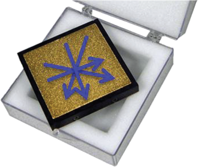
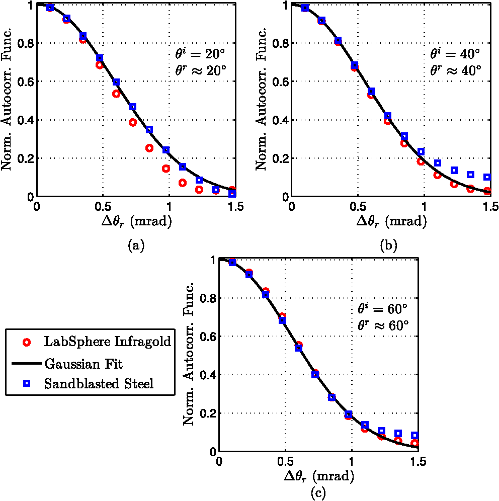
1. Introduction

Due to atmospheric turbulence and other factors, it is seldom possible to create a point source beacon at a target. The extended beacons that are created instead have intensity profiles with finite spatial extents and varying degrees of spatial coherence. It is important to model these extended beacons accurately, identify their key parameters, and develop an understanding of how they affect the overall performance of an adaptive optics (AO) system. Gaussian Schell-model (GSM) beams/sources have been used extensively in the literature to represent partially coherent light sources.¹^–⁴ Techniques for simulating such fields have been discussed by Gbur⁵ and Xiao et al.⁶ Further, it has been shown that GSM beams retain their GSM form to a good approximation even after propagation through atmospheric turbulence.⁷^–⁹ GSM beams are described by an average Gaussian intensity function and a Gaussian normalized autocorrelation function.¹⁰ The use of Gaussian functions makes the model analytically tractable.

Korotkova et al.¹¹ developed an analytical model for the scattering of a Gaussian beam from a rough-surface target. Their analysis followed two different approaches: the first used Goodman’s technique¹² of modeling the rough surface as reflection coefficients, while the other used a rough-surface phase screen model and Rytov perturbation theory. Both models yielded identical results. At normal incidence, for a surface characterized by a Gaussian height distribution and a Gaussian autocorrelation function, the far-zone scattered-field autocorrelation function followed a GSM form in the paraxial regime. The physics of the laser-target interaction, such as masking, shadowing, multiple reflections, etc., are not captured in an effects model such as those employed by Korotkova et al. Given that the GSM form is very convenient to use, it is worth investigating the validity of the model for different scattering scenarios of interest, such as non-Gaussian surfaces and off-normal illumination. Only a full-wave computational technique, such as the method of moments (MoM), can accurately evaluate the scattered field by capturing all aspects of the laser-target interaction.

The MoM technique has been used traditionally to predict plane-wave scattering from rough surfaces.¹³^–¹⁵ Scattering of an incident Gaussian beam by a perfectly conducting rough surface using full-wave methods was first investigated by Collin.¹⁶ Jacobs et al.¹⁷ used the MoM to study the absorption, transmission, and scattering characteristics of a rough resistive sheet when illuminated by a Gaussian beam. Wang et al.¹⁸ used the Kirchhoff scalar scattering approximation and the plane-wave spectrum representation of electromagnetic fields to study the characteristics of scattered radiation from dielectric surfaces illuminated by a Gaussian beam. The purpose of this work is to apply the MoM technique to evaluate the scattered field from a rough impedance surface when illuminated by a fully coherent Gaussian beam. The simulations reveal several interesting features of the scattered radiation that have not been discussed previously. Two rough-surface targets with different roughness statistics are analyzed. The simulation results are verified by experimental measurements using the Complete Angle Scatter Instrument (CASI).¹⁹ In this work, a one-dimensional (1-D) rough surface model (i.e., the rough impedance surface and illumination are assumed to be invariant in the $z$ direction) is considered for computational convenience. It should be noted that light scattered from 1-D surfaces shows the same physical behavior as light scattered from two-dimensional (2-D) surfaces.²⁰ The mechanisms that are not captured in 1-D analysis are cross-polarized scattering and out-of-plane scattering.²⁰ Note that for the real-world surfaces analyzed in this research, the scattering measurements showed that the cross-polarized scattering was negligible.

Section 2 discusses the mathematical formulation and implementation of the MoM. The process of characterization of the sample targets is described in Sec. 3. Section 4 discusses the validity of using the GSM form for extended beacon studies based on the results from the simulations. Finally, a summary of the findings and future research directions are presented in Sec. 5.

2. Methodology

The scattering geometry assumed in the analysis is shown in Fig. 1. The rough impedance surface is denoted by the function $h (x)$ , with mean, standard deviation and correlation length equal to 0, $σ_{h}$ , and $l_{h}$ , respectively. Note that, in this context, $h (x)$ is one instance of a random surface drawn from an ensemble of random surfaces. It is assumed that the first and second derivatives of $h (x)$ exist. The statistical distributions of $h (x)$ are discussed in Sec. 3. The surface is illuminated by a fully coherent Gaussian beam and the scattered radiation is observed in the far field. The incident radiation is assumed to be ${TM}^{z}$ ( $s$ -polarized). The results for the ${TE}^{z}$ polarization, not shown, are similar.

Fig. 1

Scattering geometry of a one-dimensional, rough impedance surface (i.e., the surface and source excitation are invariant in the $z$ direction). The medium below the rough interface has a permittivity of $ε$ and a permeability of $μ$ . The medium above the rough interface is vacuum.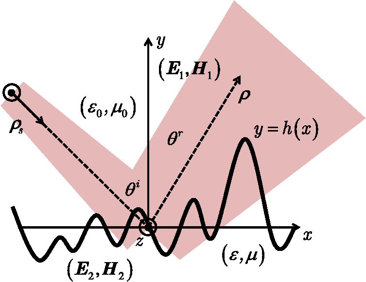

2.1.

Derivation of Coupled Electric Field Integral Equations

In accordance with the surface equivalence principle,²¹ the original scattering problem can be replaced by equivalent exterior and interior problems. In the equivalent exterior problem, the boundary is replaced by equivalent electric $(J_{1} = \hat{n} \times H_{1})$ and magnetic $(K_{1} = E_{1} \times \hat{n})$ surface currents, which reproduce the fields in region 1 in combination with the original source. Note that the electric field in region 1 is $E_{1} = E^{inc} + E^{s}$ , where $E^{inc}$ and $E^{s}$ are the incident and scattered electric fields, respectively; and the magnetic field is $H_{1}$ . Here, $\hat{n}$ is the unit normal vector pointing into region 1. Null fields are produced in region 2, which allows that region to be replaced with any desired material. It is convenient to replace region 2 with a vacuum, thus yielding currents that radiate in unbounded space (and permitting use of the free-space Green’s function²¹^–²³). In the equivalent interior problem (opposite the exterior problem), the boundary is replaced with equivalent electric $(J_{2} = - \hat{n} \times H_{2})$ and magnetic $(K_{2} = E_{2} \times - \hat{n})$ surface currents, which reproduce the fields $E_{2}$ and $H_{2}$ in region 2. Null fields are produced in the exterior region, thus permitting region 1 to be replaced with any desired material. It is convenient to replace region 1 with $ε$ and $μ$ yielding currents that radiate in unbounded space. The continuity of transverse electric and magnetic fields at the rough interface implies that $J_{1} = - J_{2} = J$ and $K_{1} = - K_{2} = K$ , yielding a system of coupled electric field integral equations, namely

Eq. (1)

\hat{n} \times E^{inc} = - K - \hat{n} \times {\frac{η_{0}}{j k_{0}} (\nabla_{t} \nabla_{t} \cdot A_{1} + k_{0}^{2} A_{1}) - \nabla_{t} \times F_{1}}_{S^{+}} 0 = K - \hat{n} \times {\frac{η}{j k} (\nabla_{t} \nabla_{t} \cdot A_{2} + k^{2} A_{2}) - \nabla_{t} \times F_{2}}_{S^{-}},

where the magnetic vector potential

A

and electric vector potential

F

are

Eq. (2)

A_{β} (ρ) = \frac{1}{4 j} \int_{C} J (ρ^{'}) H_{0}^{(2)} (k_{β} | ρ - ρ^{'} |) d ρ^{'} F_{β} (ρ) = \frac{1}{4 j} \int_{C} K (ρ^{'}) H_{0}^{(2)} (k_{β} | ρ - ρ^{'} |) d ρ^{'} .

Here,

k_{β} = {\begin{array}{l} k_{0} & β = 1 \\ k & β = 2 \end{array};

S^{+}

and

S^{-}

denote that the bracketed expressions are evaluated an infinitesimal distance above and below the rough interface, respectively;

η = \sqrt{μ / ε}

,

η_{0} = \sqrt{μ_{0} / ε_{0}}

,

k

, and

k_{0}

are the intrinsic impedances and wavenumbers of the medium below the rough interface and vacuum, respectively;

ρ^{'}

is a vector that points from the origin to any point on the surface; and

ρ

is a vector that points from the origin to the observation point. In the context of the above expressions,

ρ \in C

, where

C

is the parameterized rough surface contour. Note that the unknowns in Eq. (1) are

J

and

K

. The 2-D, free-space Green’s function is

G (ρ | ρ^{'}) = \frac{1}{4 j} H_{0}^{(2)} (k | ρ - ρ^{'} |)

, where

H_{0}^{(2)}

is the zeroth-order Hankel function of the second kind.²⁴

2.2.

Impedance Boundary Condition

The system of coupled electric field integral equations in Eq. (1) can be solved using the MoM; however, this is extremely prohibitive. Because the rough surfaces of interest are very large compared to the wavelength of the field, the size of the resulting matrix equation, formed by discretizing Eq. (1), is extremely large, making computation of the solution very difficult. However, if $R_{\min} ≫ δ$ (where $R$ is the radius of curvature and $δ$ is the skin depth), then an approximate impedance boundary condition (IBC) can be used to reduce Eq. (1) to a single equation with one unknown. This reduces the size of the matrix equation by a factor of 4. The limits of applicability of the IBC can be found in Yuferev et al.²⁵ If the IBC is valid (which it is for the surfaces analyzed in this research), the electric and magnetic surface currents are related by

Eq. (3)

K = η J \times \hat{n} .

Substituting Eq. (3) into the first equation in Eq. (1), specializing the resulting expression to the ${TM}^{z}$ polarization case, and simplifying yields the desired electric field integral equation:

Eq. (4)

E_{z}^{inc} = η J_{z} + j k_{0} η_{0} A_{z} + {(\frac{\partial F_{y}}{\partial x} - \frac{\partial F_{x}}{\partial y})}_{S +} .

Substituting in the simplified expressions for the electric and magnetic vector potentials, we get

Eq. (5)

E_{z}^{inc} (x, y) = η J_{z} + \frac{k_{0} η_{0}}{4} \int_{C} J_{z} (x^{'}) H_{0}^{(2)} (k_{0} R) \sqrt{1 + {[h^{'} (x^{'})]}^{2}} d x^{'} + \frac{k_{0} η}{4 j} \int_{C} h^{'} (x^{'}) J_{z} (x^{'}) (\frac{x - x^{'}}{R}) H_{1}^{(2)} (k_{0} R) d x^{'} - \frac{k_{0} η}{4 j} \int_{C} J_{z} (x^{'}) (\frac{y - y^{'}}{R}) H_{1}^{(2)} (k_{0} R) d x^{'},

where

R = \sqrt{{(x - x^{'})}^{2} + {(y - y^{'})}^{2}}

,

H_{1}^{(2)}

is a first-order Hankel function of the second kind, and

h (x^{'})

is the first derivative of the surface height function

h (x^{'})

.

2.3.

MoM Solution

In this analysis, the MoM is used to solve Eq. (4) for the unknown electric current. The MoM consists of two steps—expansion and testing. In the expansion step, a set of basis functions with unknown weights are chosen to expand the unknown current. The resulting system is then tested using another set of functions to solve for the unknown expansion weights. Note that at least first-order differentiability is required for basis and testing functions to overcome the Green’s function source-point singularity [ $H_{1}^{(2)} (x) \sim 1 / x$ as $x \to 0$ ];²¹ thus, pulse (rectangular) basis and delta testing functions will suffice. Substitute $J_{z} (x^{'}) = \sum_{n = 1}^{N} α_{n} f_{n} (x^{'})$ into Eq. (5), where $α_{n}$ are the unknown, complex basis function weights and $f_{n}$ is a unit pulse defined over cell $n$ , namely

Eq. (6)

f_{n} (x) = {\begin{array}{l} 1 & if x \in cell n \\ 0 & else \end{array} .

Then, testing the resulting equation [i.e., $\int_{C} δ (x - x_{m}) {\cdot} d x$ ] and simplifying yields

Eq. (7)

E_{z}^{inc} (x_{m}, y_{m}) = η α_{n} δ_{m n} + \frac{k_{0} η_{0}}{4} \sum_{n = 1}^{N} α_{n} \int_{cell n} H_{0}^{(2)} (k_{0} R_{m}) \sqrt{1 + {[h^{'} (x^{'})]}^{2}} d x^{'} - \frac{k_{0} η}{4 j} \sum_{n = 1}^{N} α_{n} \int_{cell n} \cos ϕ_{m} H_{1}^{(2)} (k_{0} R_{m}) \sqrt{1 + {[h^{'} (x^{'})]}^{2}} d x^{'},

where

Eq. (8)

R_{m} = \sqrt{{(x_{m} - x^{'})}^{2} + {(y_{m} - y^{'})}^{2}} \cos ϕ_{m} = \frac{(y_{m} - y^{'}) - (x_{m} - x^{'}) h^{'} (x^{'})}{R_{m} \sqrt{1 + {[h^{'} (x^{'})]}^{2}}},

where

δ_{m n}

is the Kronecker delta function, and

x_{m}

is the midpoint of the

m

’th pulse basis function cell. Recall that

y = h (x)

, implying that

y_{m} = h (x_{m})

. Equation (7) is a discretized version of Eq. (5). Note that the unknowns (i.e.,

α_{n}

) are no longer inside the integrals. The incident field, a Gaussian beam that is invariant in the

z

direction, is derived using the techniques employed by Andrews et al. for three-dimensional (3-D) Gaussian beams.²⁶ The incident field evaluated at the rough surface is given by

Eq. (9)

E_{z}^{inc} (x_{m}, y_{m}) = \exp [- \frac{1}{2} \frac{(\frac{2}{w_{0}^{2}} + j \frac{k_{0}}{F_{0}}) {(x_{m} \cos θ^{i} + y_{m} \sin θ^{i})}^{2}}{1 + (\frac{1}{F_{0}} - j \frac{2}{k_{0} w_{0}^{2}}) (ρ_{s} + x_{m} \sin θ^{i} - y_{m} \cos θ^{i})}] \frac{e^{- j k_{0} ρ_{s}} e^{- j k_{0} (x_{m} \sin θ^{i} - y_{m} \cos θ^{i})}}{\sqrt{1 + (\frac{1}{F_{0}} - j \frac{2}{k_{0} w_{0}^{2}}) (ρ_{s} + x_{m} \sin θ^{i} - y_{m} \cos θ^{i})}},

where

θ^{i}

is the angle of incidence,

ρ_{s}

is the distance from the source plane to the rough surface origin,

w_{0}

is the

1 / e

radius of the beam in the source plane, and

F_{0}

is the phase-front radius of curvature.

Equation (7) can now be written in matrix form as

Eq. (10)

[Z_{m n}] [α_{n}] = [E_{m}^{inc}] .

Note that because of the singularity in the Hankel functions as

R \to 0

(Green’s function source-point singularity), the diagonal terms of the impedance matrix

[Z_{m n}]

must be handled carefully. This is done by using the small argument approximations of the Hankel functions. Since the cell sizes of the pulse basis functions are small compared to the wavelength, a further simplification to the impedance matrix elements can be made by approximating the integrals with the rectangular area under the appropriate cell.²¹^,²² When these steps are taken, the elements of the impedance matrix are

Eq. (11)

Z_{m n} = {\begin{array}{l} \frac{k_{0} η_{0}}{4} H_{0}^{(2)} (k_{0} R_{m n}) Δ_{n} - \frac{k_{0} η}{4 j} H_{1}^{(2)} (k_{0} R_{m n}) \cos ϕ_{m n} Δ_{n} & m \neq n \\ \frac{η}{2} + \frac{k_{0} η_{0}}{4} Δ_{n} [1 - j \frac{2}{π} \log (\frac{γ k_{0} Δ_{n}}{4 e})] & m = n \end{array},

where

γ

is the Euler constant and

Δ_{n}

is the width of the

n

’th pulse basis function cell.

The elements of $[Z_{m n}]$ are remarkably physical. For instance, element $m$ , $n$ models how the source located in cell $n$ affects the field observed at point $(x_{m}, y_{m})$ . Due to electromagnetic reciprocity, the impedance matrix is symmetrical. Physical intuition dictates that the closer the source and observation point are to each other, the more significant the coupling between the two is. This intuition is captured in the impedance matrix, which although generally full, is highly diagonal, i.e., the “self” terms (source and observer at same location) are dominant. If the surface is perfectly reflecting ( $η = 0$ ) or perfectly conducting, the impedance matrix contains only the terms involving $η_{0}$ . The terms involving $η$ are correction terms accounting for a surface with a nonzero impedance. Note that for metals that are highly reflective, the $η$ terms are significantly smaller than the terms involving $η_{0}$ .

The scattered field at an observation point $(x, y)$ in the far zone can be expressed as

Eq. (12)

E_{z}^{s} = \frac{k_{0} \exp [j (\frac{π}{4} - k_{0} ρ)]}{\sqrt{8 π k_{0} ρ}} [- η_{0} \sum_{n} α_{n} Δ_{n} e^{j k_{0} (x_{n} \sin θ^{r} + y_{n} \cos θ^{r})} + η \sum_{n} α_{n} \cos ϕ_{n} Δ_{n} e^{j k_{0} (x_{n} \sin θ^{r} + y_{n} \cos θ^{r})}],

where

θ^{r}

is the observation angle,

(x_{n}, y_{n})

is the midpoint of the

n

’th pulse basis function cell,

ρ

is the distance to the far-field observation point

(x, y)

, and

R_{n}

and

\cos ϕ_{n}

are

Eq. (13)

R_{n} = \sqrt{{(x - x_{n})}^{2} + {(y - y_{n})}^{2}} \cos ϕ_{n} = \frac{(y - y_{n}) - (x - x_{n}) h^{'} (x_{n})}{R_{n} \sqrt{1 + {[h^{'} (x_{n})]}^{2}}} .

The interested reader is referred to Harrington,²³ which outlines the methodology used in the derivation of Eq. (12).

3. Characterization of Standard Targets Based on Profilometer Measurements

In order to obtain a more practical set of simulation results, roughness parameters of two standard rough-surface targets, sandblasted steel and LabSphere Infragold (LabSphere, North Sutton, New Hampshire),²⁷ were used in this analysis. These targets measured $5.08 \times 5.08 {cm}^{2}$ and were highly reflective. The targets were first cleaned with liquid nitrogen and methanol. Using a KLA Tencor Alpha-Step IQ surface profiler (Millice, Singapore),²⁸ four scans were taken (each 1 cm in length) for each target in the manner depicted in Fig. 2. The step size for the scans was 0.2 μm. This generated four data sets of 50,000 surface points for both targets. The data sets were then analyzed to determine the autocorrelation and surface roughness statistics of the targets. A stretched exponential (SE) function was used to fit the autocorrelation data.²⁹ This function is used extensively in lithography and takes the following form:

Eq. (14)

R (τ) = σ_{h}^{2} \exp [- {(\frac{| τ |}{l_{h}})}^{2 α}],

where

σ_{h}^{2}

is the variance of the surface heights,

l_{h}

is the correlation length of the surface, and

α

is the roughness exponent. Figure 3 shows SE function fits to the autocorrelation data derived from the profilometer measurements.

Fig. 2

LabSphere Infragold target with profilometer scan directions annotated.

Fig. 3

SE nonlinear least-squares fits to measured autocorrelation data. (a) LabSphere Infragold normalized autocorrelation function fit; and (b) sandblasted steel normalized autocorrelation function fit.

For the surface height statistics, the following SE probability density function (PDF) was used:

Eq. (15)

p_{H} (h) = A \exp [- {(\frac{| h - μ |}{\sqrt{2} σ_{h}})}^{α}],

where

μ

is the mean surface height and

A

is a constant that ensures the PDF integrates to unity. Note that

μ

,

σ_{h}

, and

α

were determined via curve fitting. Once the statistical parameters of the surfaces were determined, these parameters were used to generate several independent SE-SE surface realizations in the manner outlined by Yura and Hanson.³⁰ Figure 4 shows the results of this process comparing the simulated SE-SE surface statistics with the measured profilometer data.

Fig. 4

Simulated and measured surface statistics results. (a) surface height PDF; (b) surface slope PDF; and (c) normalized autocorrelation function of surface heights.

4. Simulation Results

4.1.

Experimental Validation of Simulated Scattering Data

Simulations were performed to compute the statistical scattered radiation in the far field for the two rough targets when illuminated at different angles of incidence. In these simulations, the rough-surface statistics obtained from the characterization procedure discussed in Sec. 3 were used. The simulation results were verified against experimental measurements from the CASI. To ensure a high-fidelity validation of the MoM simulation results, the CASI incident laser beam parameters and the source-to-sample distance were carefully determined and used in the simulations. From this analysis of the CASI, a unit-amplitude, collimated Gaussian beam at a source-to-target distance of 185 cm and waist of 1.5 mm was determined to best match the incident field of the experimental apparatus. A photograph of the CASI is shown in Fig. 5. The operating wavelength for the measurements and simulations was 3.39 μm.

Fig. 5

The experimental setup for the Schmitt Measurement Services CASI. The white ray, from the lower right, represents the laser beam path incident on the white sample (laser sources not shown). The detector, positioned on a motorized rotating arm, is located at the end of the white ray leaving the sample. Any incident and observation geometry is possible by rotating the sample (either in azimuth or elevation) in combination with the detector.

The CASI incident beam spot size on the samples underfilled the field of view of its detector. Hence, one would expect to observe a large number of speckles at the detector. To handle this, the CASI uses an integrating lens that effectively averages over the received speckle pattern. This was realized in simulation by assuming that the spatial averaging over one speckle pattern performed by the CASI was equivalent to averaging over the speckle patterns predicted from numerous statistically identical rough-surface realizations (i.e., “spatial ergodicity”).³¹ For the simulation statistics to converge to within 0.1%, 400 surface realizations were required and used. Figure 6 shows the average scattered irradiances, or $〈 E_{z}^{s} (θ^{i} | θ^{r}) E_{z}^{s *} (θ^{i} | θ^{r}) 〉$ , and the measured scattered powers from the LabSphere Infragold sample versus the observation angle $θ^{r}$ for incident angles $θ^{i} = 20 deg$ , 40 deg, and 60 deg, respectively. Both the simulated (solid black traces) and measured (solid gray traces) results are shown on the same plots, but with different scales. The simulated results trend well with the measured data, with specular peaks in the same location and with roughly the same width. It should be noted that the CASI measures the scattered power from a 2-D surface, whereas the simulation predicts the scattered power from a 1-D surface. In similar previous work, Knotts et al.³² suggested that the difference between the measured and simulated data can be attributed to higher-order statistics of the rough surface that are not accurately modeled in simulation. Despite these differences, the simulated and measured results compare quite well.

Fig. 6

Average scattered irradiance and measured scattered power versus observation angle $θ^{r}$ for the LabSphere Infragold sample. The average scattered irradiance was calculated by averaging the scattered irradiance, predicted using the MoM, over 400 independent surface realizations generated using the LabSphere Infragold’s measured roughness statistics. The scattered power measurements were taken using the CASI. The angles of incidence are (a) 20 deg, (b) 40 deg, and (c) 60 deg.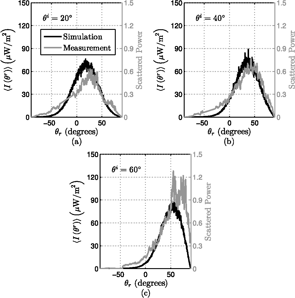

4.2.

Validation of the GSM Form for Surfaces with Gaussian Height Distributions and Gaussian Autocorrelation Functions Illuminated at Normal Incidence

Earlier studies¹¹ have shown that if a rough surface with Gaussian statistics is illuminated at normal incidence, the scattered field autocorrelation function follows a GSM form. This implies the average scattered irradiance and the normalized autocorrelation function are both Gaussian and separable. Further, the normalized autocorrelation function depend on the difference of observation angles. In order to validate this, MoM simulations were performed for very rough and smooth-to-moderately rough surfaces.

4.2.1.

Very rough surfaces

For these simulations, 1000 independent realizations of a rough surface following Gaussian statistics were generated. The surface height standard deviation and correlation length for these simulated surfaces were 11 and 117 μm, respectively, corresponding to the measured statistics of the LabSphere Infragold target. The operating wavelength was, again, 3.39 μm. Figure 7(a) shows the average far-field scattered irradiance for normal incidence as the observation angle is varied from $- 90 \deg$ to 90 deg. The average scattered irradiance is very near Gaussian. Figure 7(b) and 7(c) shows the normalized autocorrelation functions calculated around 0 deg (normal) and 30 deg observation directions, respectively. The normalized autocorrelation function of the scattered field is calculated as

Eq. (16)

μ (θ^{r}, θ^{r} + Δ θ^{r}) = \frac{| 〈 E_{z}^{s} (θ^{r}) E_{z}^{s *} (θ^{r} + Δ θ^{r}) 〉 |}{\sqrt{〈 E_{z}^{s} (θ^{r}) E_{z}^{s *} (θ^{r}) 〉} \sqrt{〈 E_{z}^{s} (θ^{r} + Δ θ^{r}) E_{z}^{s *} (θ^{r} + Δ θ^{r}) 〉}},

where the functional dependence on

θ^{i}

has been omitted for convenience. Like the average scattered irradiance, the normalized autocorrelation functions are very near Gaussian; however, the two functions have different widths, suggesting that

μ

is not a function of

Δ θ^{r}

alone. Note that the scattered field is correlated for small

Δ θ^{r}

. An analytical model based on the physical-optics approximation developed by Hyde et al.³³ shows that

μ

depends on the difference of the projected angles

\sin θ_{1}^{r}

and

\sin θ_{2}^{r}

. Further, since the scattered field is correlated over small angular separations, it was shown that the normalized autocorrelation function can be approximated as a function of only

Δ θ^{r}

by dividing it by

\cos θ^{r}

. This finding verifies the work of Korotkova et al.,¹¹ whose analysis, restricted to the paraxial regime, showed that

μ

depended on the difference of observation-plane coordinates. Nevertheless, since

μ

is not a function of

Δ θ^{r}

alone, the scattered field autocorrelation function does not adhere to the GSM definition in general. Note that the widths of the normalized autocorrelation functions are on the order of

λ / D

, where

λ

is the wavelength and

D

is the spot size on the target. This is consistent with earlier theories developed by Goodman¹² and Korotkova et al.¹¹

Fig. 7

Average far-field scattered irradiance and normalized autocorrelation functions at normal incidence for a simulated rough Gaussian surface with a height standard deviation of 11 μm and correlation length of 117 μm. (a) Average scattered irradiance; (b) and (c) are the normalized autocorrelation function plots for observation at 0 deg and 30 deg, respectively. The scattered irradiance profile and the normalized autocorrelation function plots have a distinctive Gaussian shape. Note that the widths of the traces in (b) and (c) are different, suggesting that $μ$ is not a function of $Δ θ^{r}$ al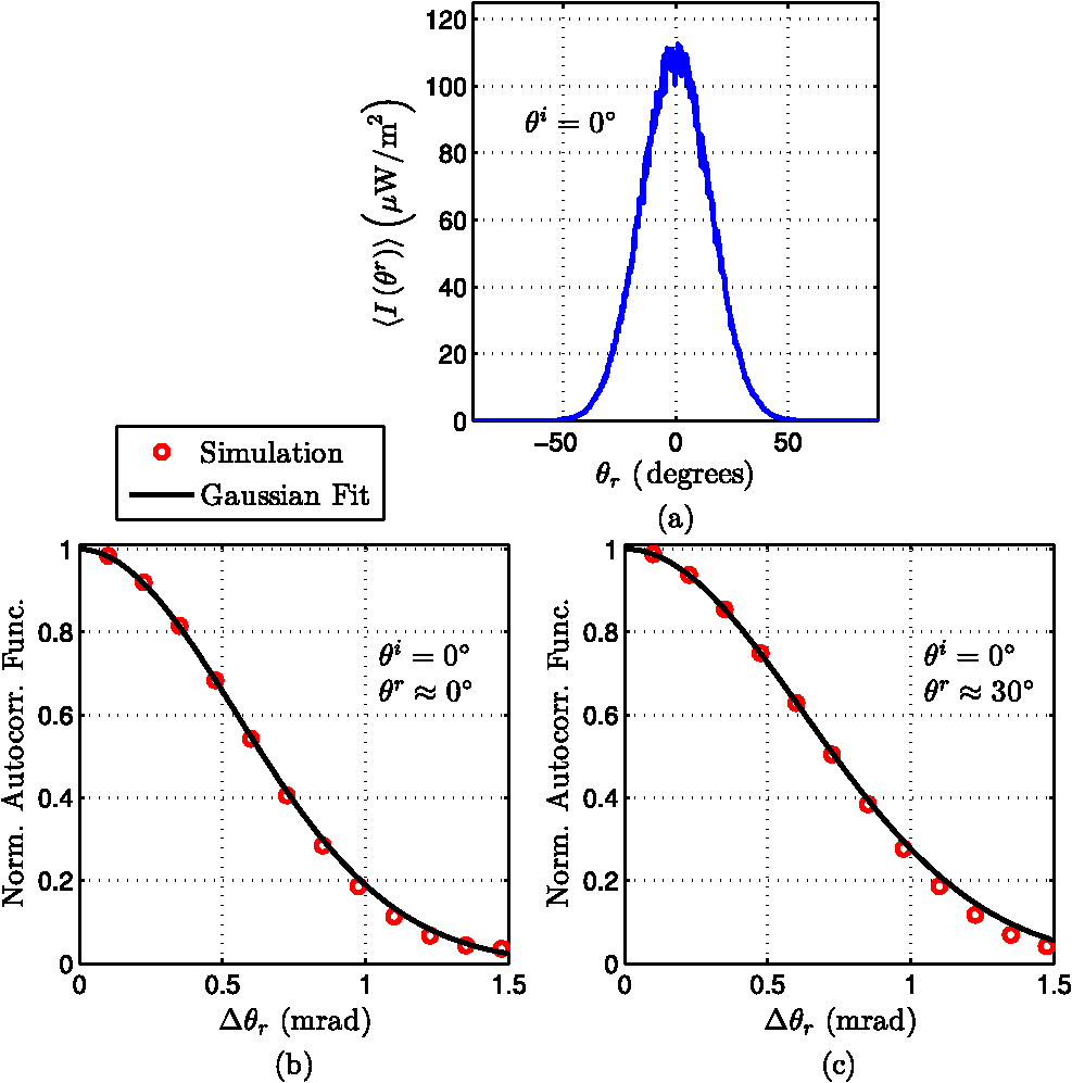one.

4.2.2.

Smooth to moderately rough surfaces

The normalized autocorrelation function can no longer be described by a Gaussian function as the surface gets smoother with respect to wavelength. This behavior was noted by Goodman for near-field scattering observed just above the rough surface.³⁴ Figure 8 shows the normalized autocorrelation functions for observation around the specular direction for a Gaussian surface at normal incidence when the surface height standard deviation is varied. The correlation lengths of the simulated surfaces were $8 λ$ . When the surface roughness is much smaller than the wavelength (i.e., $σ_{h} = 0.05 λ$ and $0.1 λ$ ), the normalized autocorrelation functions are marked by non-Gaussian shapes and approach an asymptotic value for large separation angles. This behavior at large separation angles is due to a nonzero mean scattered field $〈 E_{z}^{s} (θ^{i} | θ^{r}) 〉$ and physically denotes the existence of a strong specular component in the scattered wave.³⁴ As the surface roughness increases to $0.25 λ$ , the normalized autocorrelation function starts assuming a Gaussian shape and the horizontal asymptote disappears, implying that the mean scattered field is zero, as in the very rough surface analysis discussed previously.

Fig. 8

Normalized autocorrelation functions of the far-zone scattered-field at normal incidence and normal observation for simulated rough Gaussian surfaces as surface roughness is varied. For $σ_{h} = 0.05 λ$ and $σ_{h} = 0.1 λ$ , the normalized autocorrelation functions are non-Gaussian and approach an asymptotic value for large separation angles. The normalized autocorrelation function is very nearly Gaussian for 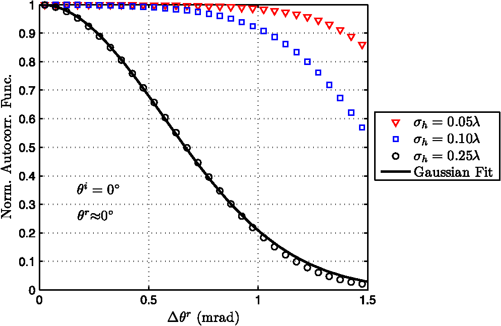$σ_{h} = 0.25 λ$ .

4.3.

Validation of GSM Form for Scattering from Sample Targets

For these simulations, the MoM was used to predict the scattered radiation in the far field for 400 independent surface realizations using the measured statistics of LabSphere Infragold and sandblasted steel. Incident angles of 20 deg, 40 deg, and 60 deg were used in the simulations. Figure 9 shows the far-field average scattered irradiances for both samples for different angles of incidence. Similarities are observed in the scattering from both samples. The scattering is maximum in the specular direction even at $θ^{i} = 60 \deg$ . Masking, shadowing, and multiple scattering effects do not appear to be significant in either target. The statistical analysis of the profilometer measurements suggested that both LabSphere Infragold and sandblasted steel had surface height distributions and correlation functions that were non-Gaussian. Figure 9 suggests that the non-Gaussian nature of the surfaces makes the angular scattered irradiance also non-Gaussian. This non-Gaussian behavior is more apparent at higher angles of incidence.

Fig. 9

Average scattered irradiances for LabSphere Infragold and sandblasted steel. Angles of incidence are (a) 20 deg, (b) 40 deg, and (c) 60 deg.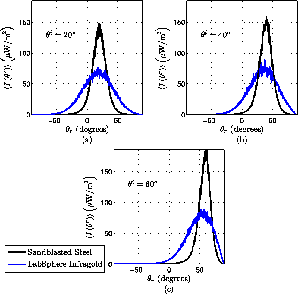

The behavior of the normalized autocorrelation functions was also examined using the simulated data. The normalized autocorrelation functions for an incident angle of 20 deg and different observation directions are shown in Fig. 10. The normalized autocorrelation functions have Gaussian shapes, but the angular widths of the functions are different, suggesting the same behavior of $μ$ that was observed earlier in Sec. 4.2.1. Figure 11 shows the normalized autocorrelation functions for both samples in the specular direction for three different angles of incidence. It is evident from the plots that the angular width of the normalized autocorrelation function for observation near the specular angle (being nearly the same in all three plots) is independent of incident direction. This finding is consistent with Goodman’s classic result.¹² Note that the width of the normalized autocorrelation function physically denotes the average angular extent of a speckle.

Fig. 10

Normalized autocorrelation functions of the far-zone scattered field of LabSphere Infragold and sandblasted steel in different observation directions. In all the plots, the angle of incidence is 20 deg. The observation directions are (a) 0 deg (normal), (b) 20 deg (specular), and (c) 40 deg. The normalized autocorrelation functions are nearly Gaussian, with very similar angular widths for both samples. Note that the angular widths are different depending on the observation direction.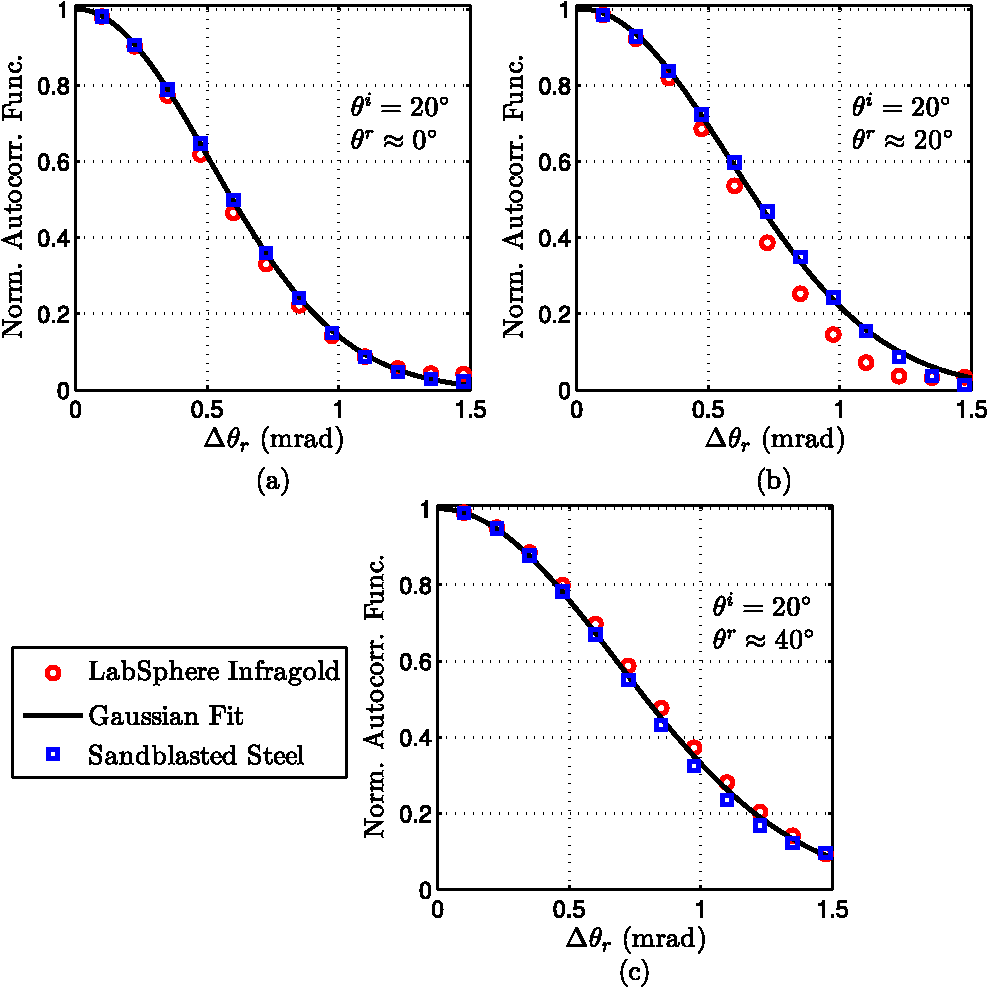

Fig. 11

Normalized autocorrelation functions of the far-zone scattered field of LabSphere Infragold and sandblasted steel when observation is in the specular direction. The angles of incidence are (a) 20 deg, (b) 40 deg, and (c) 60 deg. The angular widths for all three cases are nearly identical.

5. Conclusion

In this paper, the scattering of a fully coherent Gaussian beam from a 1-D rough impedance surface was examined using a full-wave computational technique known as the MoM. The model used surface statistics derived from profilometer measurements of two rough metallic surface targets. The simulation results agreed well with scattering measurements from a scatterometer.

The results of this analysis have revealed several interesting aspects of scattering from rough surfaces. Contrary to the existing effects models,¹¹ which suggest a GSM form for the scattered-field autocorrelation function, the full-wave model showed several deviations from GSM behavior. The scattering behavior was different for surfaces that were very rough compared to wavelength, as opposed to surfaces that were smooth to moderately rough. For very rough surfaces, the average scattered irradiances were not, in general, Gaussian when the surface statistics were non-Gaussian. For near-normal incident angles, the average scattered irradiances were approximately Gaussian (consistent with previous literature valid only in the paraxial regime); however, for large angles of incidence, the scattered irradiances deviated significantly from Gaussian. The normalized scattered-field autocorrelation functions were generally Gaussian in shape; however, contrary to the GSM definition, they were not functions of the observation angle separation $Δ θ^{r}$ alone. When observation was in the specular direction, the widths of the normalized autocorrelation functions showed very good agreement with Goodman’s classic result. For smooth-to-moderately rough surfaces, the full-wave model showed non-Gaussian behavior for both the average scattered irradiances and the normalized autocorrelation functions. The normalized autocorrelation functions started assuming Gaussian shapes when the surface roughness was approximately $0.25 λ$ . Future work will include examination of the scattering behavior in the presence of atmospheric turbulence. The scattering from 2-D surfaces, including polarimetric effects, will also be investigated.

Acknowledgments

The authors would like to thank Dr. Brij Agrawal, director of the Adaptive Optics Center of Excellence for National Security at Naval Postgraduate School, Monterey for funding this research. A special thanks to Dr. Stephen Nauyoks and the graduate students at the Optical Scatter Lab at the Air Force Institute of Technology (AFIT) for providing the experimental data. This research was supported in part by an appointment to the Postgraduate Research Participation Program at AFIT administered by the Oak Ridge Institute for Science and Education through an interagency agreement between the U.S. Department of Energy and AFIT.

References

1.

K. DrexlerM. RoggemannD. Voelz, “Use of a partially coherent transmitter beam to improve the statistics of received power in a free-space optical communication system: theory and experimental results,” Opt. Eng., 50 (2), 025002 (2011). http://dx.doi.org/10.1117/1.3533737 OPEGAR 0091-3286 Google Scholar

2.

G. GburE. Wolf, “Spreading of partially coherent beams in random media,” J. Opt. Soc. Am. A, 19 (8), 1592 –1598 (2002). http://dx.doi.org/10.1364/JOSAA.19.001592 JOAOD6 1084-7529 Google Scholar

3.

G. GburT. Visser, “The structure of partially coherent fields,” Progr. Opt., 55 285 –341 (2010). http://dx.doi.org/10.1016/B978-0-444-53705-8.00005-9 POPTAN 0079-6638 Google Scholar

4.

O. KorotkovaL. C. AndrewsR. L. Phillips, “Model for a partially coherent Gaussian beam in atmospheric turbulence with application in Lasercom,” Opt. Eng., 43 (2), 330 –341 (2004). http://dx.doi.org/10.1117/1.1636185 OPEGAR 0091-3286 Google Scholar

5.

G. Gbur, “Simulating fields of arbitrary spatial and temporal coherence,” Opt. Express, 14 (17), 7567 –7578 (2006). http://dx.doi.org/10.1364/OE.14.007567 OPEXFF 1094-4087 Google Scholar

6.

X. XiaoD. Voelz, “Wave optics simulation approach for partial spatially coherent beams,” Opt. Express, 14 (16), 6986 –6992 (2006). http://dx.doi.org/10.1364/OE.14.006986 OPEXFF 1094-4087 Google Scholar

7.

J. C. RicklinF. M. Davidson, “Atmospheric turbulence effects on a partially coherent Gaussian beam: implications for free-space laser communication,” J. Opt. Soc. Am. A, 19 (9), 1794 –1802 (2002). http://dx.doi.org/10.1364/JOSAA.19.001794 JOAOD6 0740-3232 Google Scholar

8.

S. C. H. WangM. A. Plonus, “Optical beam propagation for a partially coherent source in the turbulent atmosphere,” J. Opt. Soc. Am., 69 (9), 1297 –1304 (1979). http://dx.doi.org/10.1364/JOSA.69.001297 JOSAAH 0030-3941 Google Scholar

9.

D. J. WheelerJ. D. Schmidt, “Spatial coherence function of partially coherent Gaussian beams in atmospheric turbulence,” Appl. Opt., 50 (21), 3907 –3917 (2011). http://dx.doi.org/10.1364/AO.50.003907 APOPAI 0003-6935 Google Scholar

10.

L. MandelE. Wolf, Optical Coherence and Quantum Optics, Cambridge University Press, New York (1995). Google Scholar

11.

O. KorotkovaL. C. Andrews, “Speckle propagation through atmospheric turbulence: effects of partial coherence of the target,” Proc. SPIE, 4723 73 –84 (2002). http://dx.doi.org/10.1117/12.476417 PSISDG 0277-786X Google Scholar

12.

J. Goodman, “Statistical properties of laser speckle patterns,” Laser Speckle and Related Phenomena, 9 –75 Springer, Berlin Heidelberg (1975). Google Scholar

13.

R. AxlineA. Fung, “Numerical computation of scattering from a perfectly conducting random surface,” IEEE Trans. Antenn. Propag., 26 (3), 482 –488 (1978). http://dx.doi.org/10.1109/TAP.1978.1141871 IETPAK 0018-926X Google Scholar

14.

M. ChenS. Bai, “Computer simulation of wave scattering from a dielectric random surface in two dimensions—cylindrical case,” J. Electromagn. Waves Appl., 4 (10), 963 –982 (1990). http://dx.doi.org/10.1163/156939390X00708 JEWAE5 0920-5071 Google Scholar

15.

A. K. FungM. F. Chen, “Numerical simulation of scattering from simple and composite random surfaces,” J. Opt. Soc. Am. A, 2 (12), 2274 –2284 (1985). http://dx.doi.org/10.1364/JOSAA.2.002274 JOAOD6 0740-3232 Google Scholar

16.

R. Collin, “Scattering of an incident Gaussian beam by a perfectly conducting rough surface,” IEEE Trans. Antenn. Propag., 42 (1), 70 –74 (1994). http://dx.doi.org/10.1109/8.272303 IETPAK 0018-926X Google Scholar

17.

E. JacobsR. Lang, “Scattering, transmission, and absorption by a rough resistive sheet—E polarization,” IEEE Trans. Antenn. Propag., 50 (11), 1567 –1576 (2002). http://dx.doi.org/10.1109/TAP.2002.803967 IETPAK 0018-926X Google Scholar

18.

M.-J. WangZ.-S. WuY.-L. Li, “Investigation on the scattering characteristics of Gaussian beam from two-dimensional dielectric rough surfaces based on the Kirchhoff approximation,” Prog. Electromagn. Res. B, 4 223 –235 (2008). http://dx.doi.org/10.2528/PIERB08010903 Google Scholar

19.

B. Balling, “A comparative study of the bidirectional reflectance distribution function of several surfaces as a mid-wave infrared diffuse reflectance standard,” Air Force Institute of Technology, (2009). Google Scholar

20.

J. T. Johnson, “Computer simulations of rough surface scattering,” Light Scattering and Nanoscale Surface Roughness, Springer Science + Business Media, New York (2007). Google Scholar

21.

A. PetersonS. RayR. Mittra, Computational Methods for Electromagnetics, IEEE Press, Piscataway, New Jersey (1998). Google Scholar

22.

R. Harrington, Field Computation by Moment Methods, IEEE Press, Piscataway, New Jersey (1993). Google Scholar

23.

R. Harrington, Time-Harmonic Electromagnetic Fields, Piscataway, New Jersey (2001). Google Scholar

24.

Handbook of Mathematical Functions with Formulas, Graphs, and Mathematical Tables, Dover Publications, New York (1972). Google Scholar

25.

S. V. YuferevN. Ida, Surface Impedance Boundary Conditions: A Comprehensive Approach, CRC Press, Boca Raton, Florida (2009). Google Scholar

26.

L. C. AndrewsR. L. Phillips, Laser Beam Propagation through Random Media, 2nd ed.SPIE Press, Bellingham, WA (2005). Google Scholar

27.

., “A guide to reflectance coatings and materials,” http://www.labsphere.com/tecdocs.aspx Google Scholar

28.

, “Alpha-step IQ surface profiler,” http://www.kla-tencor.com/surface-profiling/alpha-step-iq.html Google Scholar

29.

C. A. Mack, “Analytic form for the power spectral density in one, two, and three dimensions,” J. Micro/Nanolithogr. MEMS MOEMS, 10 (4), 040501 (2011). http://dx.doi.org/10.1117/1.3663567 JMMMHG 1932-5150 Google Scholar

30.

H. T. YuraS. G. Hanson, “Digital simulation of an arbitrary stationary stochastic process by spectral representation,” J. Opt. Soc. Am. A, 28 (4), 675 –685 (2011). http://dx.doi.org/10.1364/JOSAA.28.000675 JOAOD6 0740-3232 Google Scholar

31.

M.-J. Kimet al., “Experimental study of enhanced backscattering from one- and two-dimensional random rough surfaces,” J. Opt. Soc. Am. A, 7 (4), 569 –577 (1990). http://dx.doi.org/10.1364/JOSAA.7.000569 JOAOD6 0740-3232 Google Scholar

32.

M. E. KnottsT. R. MichelK. A. O’Donnell, “Comparisons of theory and experiment in light scattering from a randomly rough surface,” J. Opt. Soc. Am. A, 10 (5), 928 –941 (1993). http://dx.doi.org/10.1364/JOSAA.10.000928 JOAOD6 0740-3232 Google Scholar

33.

M. W. Hydeet al., “Scalar wave solution for the scattering of a partially coherent beam from a statistically rough metallic surface,” Proc. SPIE, 8550 85503A (2012). http://dx.doi.org/10.1117/12.979947 PSISDG 0277-786X Google Scholar

34.

J. W. Goodman, Speckle Phenomena in Optics: Theory and Applications, Ben Roberts & Company, Greenwood Village, Colorado (2007). Google Scholar

Biography

Santasri Basu received her BE degree in electrical engineering with honors from Jadavpur University, Kolkata, India, in 2000, and her MS and PhD degrees in electrical engineering with focus in optics from New Mexico State University, Las Cruces, New Mexico, in 2005 and 2008, respectively. From 2008 to 2011, she was a visiting assistant professor in the department of physics and optical engineering at Rose-Hulman Institute of Technology, Terre Haute, Indiana. Currently, she is a research associate at the Center for Directed Energy of the Air Force Institute of Technology in the engineering physics department. Her current research interests include rough-surface scattering, laser communications, adaptive optics, and telescope pointing and tracking. She is a member of SPIE, OSA, and DEPS.

Milo W. Hyde IV received his BS degree in computer engineering from the Georgia Institute of Technology, Atlanta, Georgia, in 2001, and his MS and PhD degrees in electrical engineering from the Air Force Institute of Technology, Wright-Patterson Air Force Base, Dayton, Ohio, in 2006 and 2010, respectively. From 2001 to 2004, he was a maintenance officer with the F-117A Nighthawk, Holloman Air Force Base, Alamogordo, New Mexico. From 2006 to 2007, he was a government researcher with the Air Force Research Laboratory, Wright-Patterson Air Force Base. He is currently an assistant professor with the Department of Electrical and Computer Engineering, Air Force Institute of Technology, Wright-Patterson Air Force Base, Ohio. His current research interests include electromagnetic material characterization, guided-wave theory, scattering, and optics. He is a member of SPIE and OSA and a senior member of IEEE.

Salvatore J. Cusumano received his BS and MS degrees in electrical engineering from the U.S. Air Force Academy (1971) and the Air Force Institute of Technology (1977), respectively. He holds a PhD in control theory from the University of Illinois (1988). He currently serves as a senior scientist at MZA, Dayton, Ohio. Prior to his current position at MZA, he taught optics and beam control at the graduate level within the engineering physics department at the Air Force Institute of Technology (AFIT). Originally, he joined AFIT as the director for the Center for Directed Energy. His research interests are manifest in his 30 years of experience working for the Air Force at Kirtland AFB in directed energy. They include resonator alignment and stabilization, intracavity adaptive optics, phased arrays, telescope control, pointing and tracking, adaptive optics, and component technology for directed energy. He holds two patents (jointly) for his work in phased arrays. He is a member of SPIE and DEPS.

Michael A. Marciniak received his BS degree in mathematics-physics from St. Joseph’s College, in Rensselaer, Indiana in 1981, the BSEE degree from the University of Missouri-Columbia in 1983, and the MSEE (electro-optics) and PhD (semiconductor physics) degrees from the Air Force Institute of Technology (AFIT) in 1987 and 1995, respectively. He is an associate professor in the Department of Engineering Physics at AFIT, with research interests in various aspects of light-matter interaction, including polarimetric scatterometry and thermal radiation of nanostructured materials, optical signatures, and high-energy-laser damage assessment. He is a member of SPIE, APS, and DEPS.

Steven T. Fiorino received BS degrees in geography and meteorology from Ohio State (1987) and Florida State (1989) universities. In addition, he holds an MS in atmospheric dynamics from Ohio State (1993) and a PhD in physical meteorology from Florida State (2002). He is a retired Air Force lieutenant-colonel with 21 years of service and currently a research associate professor of atmospheric physics within the engineering physics department at AFIT and is the director of the Center for Directed Energy. His research interests include microwave remote sensing, development of weather signal processing algorithms, and atmospheric effects on military systems such as high-energy lasers and weapons of mass destruction. He is a member of SPIE, AMS, AIAA, and DEPS.

CC BY: © The Authors. Published by SPIE under a Creative Commons Attribution 4.0 Unported License. Distribution or reproduction of this work in whole or in part requires full attribution of the original publication, including its DOI.

Citation Download Citation

Santasri Basu, Milo W. Hyde IV, Salvatore J. Cusumano, Michael A. Marciniak, and Steven T. Fiorino "Examining the validity of using a Gaussian Schell-model source to model the scattering of a fully coherent Gaussian beam from a rough impedance surface," Optical Engineering 52(3), 038001 (4 March 2013). https://doi.org/10.1117/1.OE.52.3.038001

Published: 4 March 2013

Access the abstract

JOURNAL ARTICLE
10 PAGES

DOWNLOAD PAPER SAVE TO MY LIBRARY

GET CITATION

CITATIONS

Cited by 8 scholarly publications.

Explore citations on Lens.org

KEYWORDS

Scattering

Global system for mobile communications

Gaussian beams

Laser scattering

Statistical analysis

Adaptive optics

Magnetism

1.

Introduction

2.

Methodology

Fig. 1

2.1.

Derivation of Coupled Electric Field Integral Equations

Eq. (1)

Eq. (2)

2.2.

Impedance Boundary Condition

Eq. (3)

Eq. (4)

Eq. (5)

2.3.

MoM Solution

Eq. (6)

Eq. (7)

Eq. (8)

Eq. (9)

Eq. (10)

Eq. (11)

Eq. (12)

Eq. (13)

3.

Characterization of Standard Targets Based on Profilometer Measurements

Eq. (14)

Fig. 2

Fig. 3

Eq. (15)

Fig. 4

4.

Simulation Results

4.1.

Experimental Validation of Simulated Scattering Data

Fig. 5

Fig. 6

4.2.

Validation of the GSM Form for Surfaces with Gaussian Height Distributions and Gaussian Autocorrelation Functions Illuminated at Normal Incidence

4.2.1.

Very rough surfaces

Eq. (16)

Fig. 7

4.2.2.

Smooth to moderately rough surfaces

Fig. 8

4.3.

Validation of GSM Form for Scattering from Sample Targets

Fig. 9

Fig. 10

Fig. 11

5.

Conclusion

Acknowledgments

References

Biography

Show All Keywords

Keywords/Phrases

Search In:

Publication Years