Neighborhood virtual points discriminant embedding for synthetic aperture radar automatic target recognition

Jifang Pei; Yulin Huang; Xian Liu; Jianyu Yang

doi:10.1117/1.OE.52.3.036201

7 March 2013 Neighborhood virtual points discriminant embedding for synthetic aperture radar automatic target recognition

Jifang Pei, Yulin Huang, Xian Liu, Jianyu Yang

Author Affiliations +

Optical Engineering, Vol. 52, Issue 3, 036201 (March 2013). https://doi.org/10.1117/1.OE.52.3.036201

Abstract

We propose a new feature extraction method for synthetic aperture radar automatic target recognition based on manifold learning theory. By introducing the virtual point in every sample’s neighborhood, we establish the spatial relationships of the neighborhoods. When the samples are embedded into the feature space, each sample moves toward its neighborhood virtual point, whereas the virtual points with the same class label get together, and the virtual points from different classes separate from each other. This can improve the classification and recognition performance effectively. Experiments based on the moving and stationary target acquisition and recognition database are conducted to verify the effectiveness of our method.

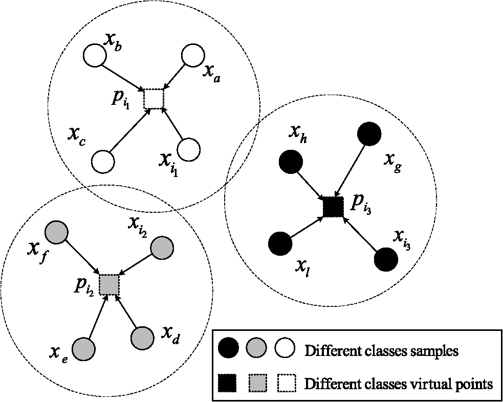
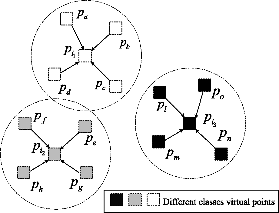
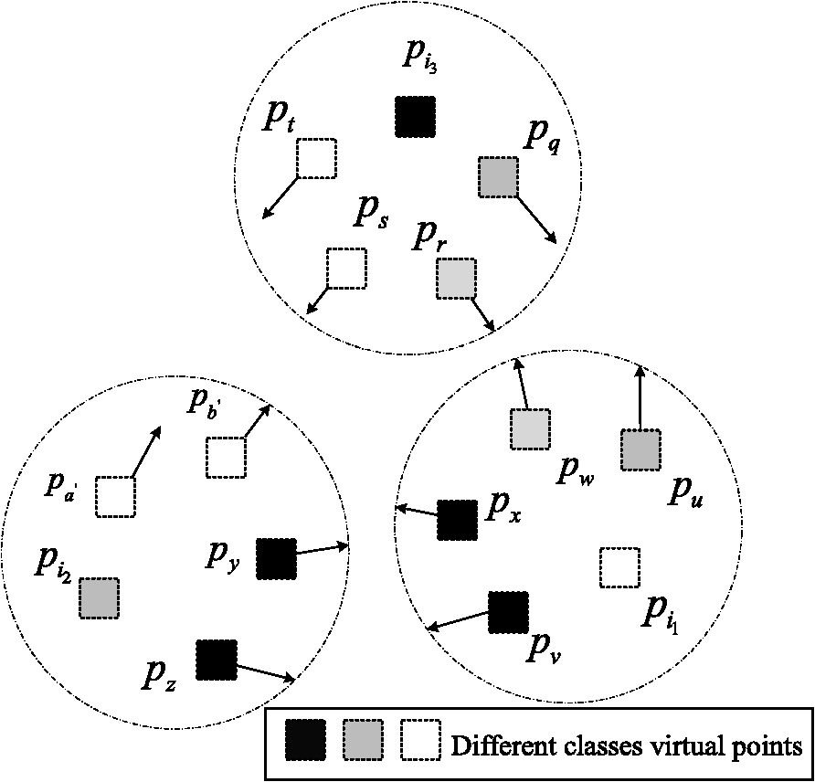
1. Introduction

Feature extraction is one of the key steps of synthetic aperture radar automatic target recognition (SAR ATR), which can reduce the dimensions of SAR images and extract the effective discriminating feature.

Generally, feature extraction methods are placed into two categories: linear and nonlinear. Classical linear methods, such as principal component analysis (PCA),¹ and linear discriminant analysis (LDA),² are based on the global linear structure of data. The best recognition rates employing PCA and LDA are higher than 80%, as shown by experiments based on the Moving and Stationary Target Acquisition and Recognition (MSTAR) database.³

With the development of the support vector machine,⁴ nonlinear feature extraction methods based on kernel tricks, such as kernel principal component analysis⁵ (KPCA) and kernel linear discriminant analysis (KLDA),⁶ have been widely applied in SAR ATR. By introducing the kernel function, those methods can solve the linearly inseparable problem of sample data to some extent. However, a main shortcoming of the kernel tricks is that the recognition performance depends on the selection of kernel settings.

Another novel nonlinear method, manifold learning,⁷ has been proposed on the premise that high-dimensional images lie on or near a low-dimensional manifold embedded in the high-dimensional space. For the purpose of seeking a low-dimensional manifold embedded in the high-dimensional data space, various manifold learning algorithms have been proposed, such as isometric feature mapping,⁸ locally linear embedding⁹ (LLE), Laplacian eigenmaps (LE),¹⁰ locality preserving projections (LPP),¹¹ neighborhood preserving embedding (NPE),¹² and orthogonal neighborhood preserving projections (ONPP).¹³

In Cai et al.,¹⁴ the LPP algorithm was introduced into inverse synthetic aperture radar target recognition, and the classification results were better than those obtained from PCA and LDA. However, LPP ignored the class information of the samples and discarded the target information from SAR images.¹⁵

The main goals of the manifold learning algorithms above are to preserve localities or similar rankings, and those methods are more appropriate for retrieval or clustering, rather than classification. By integrating the neighborhood information and class relations of samples, some supervised manifold learning methods have been proposed, including local discriminant embedding¹⁶ (LDE). Bryant¹⁷ demonstrated the application of signature manifold methods on SAR images, which has achieved considerable detection and classification results. In Venkataraman et al.,¹⁸ capturing the inter-class and intra-class variability of target shapes, coupled view and identity manifolds for shape representation was applied to target tracking and recognition. This method produced an effective classification performance. Manifold learning algorithms such as LDE only structure the adjacent graphs using samples in their neighborhoods; they ignore the spatial relationships between neighborhoods, which will restrict the classification performance.

To solve the aforementioned problems, a new feature extraction method, neighborhood virtual points discriminant embedding (NVPDE), is proposed. By introducing the virtual point in every sample’s neighborhood, relations between the samples in the neighborhood taken into account, and the spatial relationships of the neighborhoods are established. When embedded into the low-dimensional feature space, the neighborhood virtual points with the same class label, as well as every sample and its neighborhood virtual point, get together, whereas the neighborhood virtual points from different classes separate from each other. In this way, the recognition performance can be improved.

This paper is organized as follows. Section 2 details the proposed algorithm framework: samples gathered in the neighborhood, neighborhood virtual point discriminant, and objective function are detailed in Secs. 2.1 to 2.3, respectively. Section 3 shows experimental results, and Sec. 4 concludes this paper.

2. Neighborhood Virtual Points Discriminant Embedding

Let $M$ be a manifold embedded in $R^{n}$ . The training dataset is ${x_{i} \in R^{n}, i = 1, 2, \dots, N} \in M$ , and corresponding data class labels are ${y_{i} \in [1, 2, \dots, c], i = 1, 2, \dots, N}$ , where $N$ denotes the amount of training data, and $c$ denotes the class number of training data. Any subset of data points that belong to the same class is assumed to lie on a submanifold of $M$ . In NVPDE, the virtual points are introduced into the samples’ within-class neighborhoods, and then an embedding based on linear projection is constructed: $x_{i} \in R^{n} \mapsto z_{i} = V^{T} x_{i} \in R^{l}$ , $(l ≪ n)$ . Via embedding, each sample $x_{i}$ in the low-dimensional space moves toward its neighborhood virtual point $p_{i}$ , while the virtual points with the same class label get together, and the virtual points from different classes separate from each other.

2.1.

Samples Gathered in Neighborhood

We calculate the within-class neighborhood $N_{k_{1}}^{+} (x_{i})$ for each sample $x_{i}$ and select the neighborhood virtual point ${p_{i} \in R^{n}, i = 1, 2, \dots, N}$ from each neighborhood $N_{k_{1}}^{+} (x_{i})$ . Here, $N_{k_{1}}^{+} (x_{i})$ indicates the set of the $k_{1}$ nearest neighbors of the sample $x_{i}$ in the same class, $p_{i} = Φ (x_{i}, x_{a_{1}}, x_{a_{2}}, \dots, x_{a_{k_{1}}})$ , $x_{a_{1}}, x_{a_{2}}, \dots, x_{a_{k_{1}}} \in N_{k_{1}}^{+} (x_{i})$ , and $Φ (\cdot)$ is the virtual points selecting function. Here, we select the geometric center of the neighborhood $N_{k_{1}}^{+} (x_{i})$ as the neighborhood virtual point: $p_{i} = (1 / k_{1} + 1) (x_{i} + \sum_{j = 1}^{k_{1}} x_{a_{j}})$ , $i = 1, 2, \dots, N$ , $x_{a_{j}} \in N_{k_{1}}^{+} (x_{i})$ . The sample’s within-neighborhood objective function is defined as

Eq. (1)

J_{n} (V) = \sum_{i, j} {‖ z_{i} - c_{j} ‖}^{2} w_{i j}^{(n)} = \sum_{i, j} {‖ V^{T} x_{i} - V^{T} p_{j} ‖}^{2} w_{i j}^{(n)},

where

W^{(n)} = [w_{i j}^{(n)}] \in R^{N \times N}

is the sample’s within-neighborhood affinity weight matrix, which is defined as

Eq. (2)

w_{i j}^{(n)} = {\begin{array}{l} \exp {- {‖ x_{i} - p_{j} ‖}^{2}}, & if x_{i} \in N_{k_{1}}^{+} (x_{j}) or i = j \\ 0, & otherwise \end{array},

Eq. (3)

c_{j} = V^{T} p_{j} = \frac{1}{k_{1} + 1} (V^{T} x_{j} + \sum_{i = 1}^{k_{1}} V^{T} x_{a_{i}}) .

J_{n} (V)

demonstrates the spatial relationships between the samples and their respective neighborhood virtual points: The smaller the value of

J_{n} (V)

, the closer the samples are to their neighborhood virtual points. The explanation of the process of samples gathered in neighborhood is shown in Fig. 1, which shows that each sample will move toward its neighborhood virtual point.

Fig. 1

Samples’ direction in their within-class neighborhoods for NVPDE.

Referring to Eq. (1), we can infer that

Eq. (4)

J_{n} (V) = \sum_{i, j} {‖ z_{i} - c_{j} ‖}^{2} w_{i j}^{(n)} = \sum_{i, j} {‖ V^{T} x_{i} - V^{T} p_{j} ‖}^{2} w_{i j}^{(n)} = trace [\sum_{i, j} V^{T} (x_{i} - p_{j}) w_{i j}^{(n)} {(x_{i} - p_{j})}^{T} V] = trace {V^{T} [\sum_{i, j} (x_{i} w_{i j}^{(n)} x_{i}^{T} - x_{i} w_{i j}^{(n)} p_{j}^{T} - p_{j} w_{i j}^{(n)} x_{i}^{T} + p_{j} w_{i j}^{(n)} p_{j}^{T})] V} = trace [V^{T} ({X W}^{(n)} X^{T} - {X W}^{(n)} P^{T} - {P W}^{(n)} X^{T} + {P W}^{(n)} P^{T}) V],

where

X = [x_{1}, x_{2}, \dots, x_{N}] \in R^{n \times N}

,

W^{(n)} = [w_{i j}^{(n)}] \in R^{N \times N}

, and

P = [p_{1}, p_{2}, \dots, p_{N}] \in R^{n \times N}

. Let

H = [h_{j i}] \in R^{N \times N}

, where

h_{j i} = {\begin{matrix} \frac{1}{k_{1} + 1}, & if x_{j} \in N_{k_{1}}^{+} (x_{i}) or i = j \\ 0, & otherwise \end{matrix},

and

P = X H

. Thus,

Eq. (5)

J_{n} (V) = trace [V^{T} ({X W}^{(n)} X^{T} - {X W}^{(n)} H^{T} X^{T} - {X H W}^{(n)} X^{T} + {X H W}^{(n)} H^{T} X^{T}) V] = trace [V^{T} X (W^{(n)} - W^{(n)} H^{T} - {H W}^{(n)} + {H W}^{(n)} H^{T}) X^{T} V] .

Let

L^{(n)} = W^{(n)} - W^{(n)} H^{T} - {H W}^{(n)} + {H W}^{(n)} H^{T}

. Thus,

Eq. (6)

J_{n} (V) = trace (V^{T} {X L}^{(n)} X^{T} V) .

2.2.

Neighborhood Virtual Point Discriminant

Because each neighborhood virtual point $p_{i}$ is a linear combination of the samples in the neighborhood $N_{k_{1}}^{+} (x_{i})$ and $x_{i}$ , the neighborhood virtual points are essentially high-dimensional image data, as well. Therefore, they should lie on or near the low-dimensional manifold $M$ embedded in the high-dimensional space. According to the samples’ class labels, the class labels corresponding to the neighborhood virtual points ${p_{i} \in R^{n}, i = 1, 2, \dots, N}$ are ${y_{i} \in [1, 2, \dots, c], i = 1, 2, \dots, N}$ . Any subset of neighborhood virtual points that belong to the same class is assumed to lie on a submanifold of $M$ . The within-class neighborhood virtual point objective function is defined as

Eq. (7)

J_{w} (V) = \frac{1}{2} \sum_{i, j} {‖ c_{i} - c_{j} ‖}^{2} w_{i j}^{(w)} = \frac{1}{2} \sum_{i, j} {‖ V^{T} p_{i} - V^{T} p_{j} ‖}^{2} w_{i j}^{(w)},

where

W^{(w)} = [w_{i j}^{(w)}] \in R^{N \times N}

is the neighborhood virtual point affinity weight matrix, which is defined as

Eq. (8)

w_{i j}^{(w)} = {\begin{cases} \exp {- {‖ p_{i} - p_{j} ‖}^{2}}, & if p_{i} \in N_{k_{2}}^{+} (p_{j}) \\ 0, & otherwise \end{cases},

where

N_{k_{2}}^{+} (p_{j})

indicates the set of the

k_{2}

nearest neighbors of the neighborhood virtual point

p_{j}

in the same class.

$J_{w} (V)$ demonstrates the spatial relationships between the neighborhood virtual points in the same class: The smaller the value of $J_{w} (V)$ , the closer the neighborhood virtual points are to each other. The explanation of the process of neighborhood virtual point discriminant in the same class is shown in Fig. 2, which shows that the virtual points in the same class will get together.

Fig. 2

Virtual points’ direction in their within-class neighborhoods for NVPDE.

The between-class neighborhood virtual point objective function is defined as

Eq. (9)

J_{b} (V) = \frac{1}{2} \sum_{i, j} {‖ c_{i} - c_{j} ‖}^{2} w_{i j}^{(b)} = \frac{1}{2} \sum_{i, j} {‖ V^{T} p_{i} - V^{T} p_{j} ‖}^{2} w_{i j}^{(b)},

where

W^{(b)} = [w_{i j}^{(b)}] \in R^{N \times N}

is the neighborhood virtual point penalty weight matrix, which is defined as

Eq. (10)

w_{i j}^{(b)} = {\begin{cases} \exp {- {‖ p_{i} - p_{j} ‖}^{2}}, & if p_{i} \in N_{k_{3}}^{-} (p_{j}) \\ 0, & otherwise \end{cases},

where

N_{k_{3}}^{-} (p_{j})

indicates the set of the

k_{3}

nearest neighbors of the neighborhood virtual point

p_{j}

from different classes.

$J_{b} (V)$ demonstrates the spatial relationships between the neighborhood virtual points from different classes: The larger the value of $J_{b} (V)$ , the further the neighborhood virtual points are from each other. The explanation of the process of neighborhood virtual point discriminant from different classes is shown in Fig. 3, which shows that the virtual points from different classes will separate from each other.

Fig. 3

Virtual points’ direction in their between-class neighborhoods for NVPDE.

Referring to Eq. (7), we can infer that

Eq. (11)

J_{w} (V) = \frac{1}{2} \sum_{i, j} {‖ c_{i} - c_{j} ‖}^{2} w_{i j}^{(w)} = \frac{1}{2} \sum_{i, j} {‖ V^{T} p_{i} - V^{T} p_{j} ‖}^{2} w_{i j}^{(w)} = \frac{1}{2} trace [\sum_{i, j} V^{T} (p_{i} - p_{j}) w_{i j}^{(w)} {(p_{i} - p_{j})}^{T} V] = trace {V^{T} [\sum_{i, j} (p_{i} w_{i j}^{(w)} p_{i}^{T} - p_{i} w_{i j}^{(w)} p_{j}^{T})] V} = trace [V^{T} P (D^{(w)} - W^{(w)}) P^{T} V],

where

P = [p_{1}, p_{2}, \dots, p_{N}] \in R^{n \times N}

,

W^{(w)} = [w_{i j}^{(w)}] \in R^{N \times N}

,

D^{(w)} = diag (d_{11}^{(w)}, d_{22}^{(w)}, \dots, d_{N N}^{(w)})

, and

d_{i i}^{(w)} = \sum_{j} w_{i j}^{(w)}

. Let

H = [h_{j i}] \in R^{N \times N}

, where

h_{j i} = {\begin{cases} \frac{1}{k_{1} + 1}, & if x_{j} \in N_{k_{1}}^{+} (x_{i}) or i = j \\ 0, & otherwise \end{cases},

and

P = X H

. Thus,

Eq. (12)

J_{w} (V) = trace [V^{T} XH (D^{(w)} - W^{(w)}) H^{T} X^{T} V] = trace (V^{T} {X L}^{(w)} X^{T} V),

where

L^{(w)} = H (D^{(w)} - W^{(w)}) H^{T}

.

Referring to Eq. (9), we can infer that

Eq. (13)

J_{b} (V) = \frac{1}{2} \sum_{i, j} {‖ c_{i} - c_{j} ‖}^{2} w_{i j}^{(b)} = \frac{1}{2} \sum_{i, j} {‖ V^{T} p_{i} - V^{T} p_{j} ‖}^{2} w_{i j}^{(b)} = \frac{1}{2} trace [\sum_{i, j} V^{T} (p_{i} - p_{j}) w_{i j}^{(b)} {(p_{i} - p_{j})}^{T} V] = trace {V^{T} [\sum_{i, j} (p_{i} w_{i j}^{(b)} p_{i}^{T} - p_{i} w_{i j}^{(b)} p_{j}^{T})] V} = trace [V^{T} P (D^{(b)} - W^{(b)}) P^{T} V],

where

P = [p_{1}, p_{2}, \dots, p_{N}] \in R^{n \times N}

,

W^{(b)} = [w_{i j}^{(b)}] \in R^{N \times N}

,

D^{(b)} = diag (d_{11}^{(b)}, d_{22}^{(b)}, \dots, d_{N N}^{(b)})

, and

d_{i i}^{(b)} = \sum_{j} w_{i j}^{(b)}

. Let

H = [h_{j i}] \in R^{N \times N}

, where

h_{j i} = {\begin{matrix} \frac{1}{k_{1} + 1}, & if x_{j} \in N_{k_{1}}^{+} (x_{i}) or i = j \\ 0, & otherwise \end{matrix},

and

P = X H

. Thus,

Eq. (14)

J_{b} (V) = trace [V^{T} X H (D^{(b)} - W^{(b)}) H^{T} X^{T} V] = trace (V^{T} {X L}^{(b)} X^{T} V),

where

L^{(b)} = H (D^{(b)} - W^{(b)}) H^{T}

.

2.3.

Objective Function

For the purpose of classification, we expect that $J_{n} (V)$ and $J_{w} (V)$ have small values, while $J_{b} (V)$ has a large value, so that each sample in the low-dimensional space will move toward its neighborhood virtual point, while the virtual points in the same class get together, and the virtual points from different classes separate from each other. Therefore, the samples in the same class will get close, whereas the samples of different classes will separate from each other in low-dimensional space.

Let $J_{w}^{'} (V) = J_{n} (V) + J_{w} (V)$ . Referring to Eqs. (6) and (12), we can infer that

Eq. (15)

J_{w}^{'} (V) = trace (V^{T} {X L}^{(n)} X^{T} V) + trace (V^{T} {X L}^{(w)} X^{T} V) = trace [V^{T} X (L^{(n)} + L^{(w)}) X^{T} V] = trace (V^{T} {XL}^{(w)'} X^{T} V) .

Consequently, according to Eqs. (14) and (15) and Fisher’s criterion,¹⁹ the objective function of NVPDE can be formulated as

Eq. (16)

V^{*} = \underset{V}{argmax trace} (\frac{V^{T} {X L}^{(b)} X^{T} V}{V^{T} {X L}^{(w)'} X^{T} V}) .

The columns of the optimal $V$ are the generalized eigenvectors corresponding to the $l$ largest eigenvalues in

Eq. (17)

{X L}^{(b)} X^{T} v = λ {X L}^{(w)'} X^{T} v .

The NVPDE algorithm procedures are formally stated as follows:

1. Compute the weight matrices $W^{(n)}$ , $W^{(w)}$ , and $W^{(b)}$ according to Eqs. (2), (8), and (10).
2. According to Eqs. (14) and (15), compute the matrices $L^{(b)}$ and $L^{(w)'}$ , and then solve the optimal embedding $V$ according to Eq. (17).
3. Feature extraction: Given a testing sample $x_{t}$ , the extracted feature based on NVPDE is $z_{t} = V^{T} x_{t}$ , where $z_{t} \in R^{l}$ .

Concerning the computational complexity of the proposed algorithm, we note that the complexity of searching $k$ nearest neighbors for all the samples and neighborhood virtual points is $O (n N^{2})$ . The complexity of calculating the elements of weight matrices is $O (n N)$ . The complexity of computing the matrices $L^{(b)}$ and $L^{(w)'}$ is $O (N^{3})$ , and the complexity of solving the generalized eigenvalue decomposition problem is $O (n^{3})$ . In most cases, the number of training samples is less than the dimension of the training sample $(N < n)$ . Therefore, like most other feature extraction methods, the computational bottleneck of NVPDE is solving the generalized eigenvalue problem, whose computational complexity is $O (n^{3})$ .

3. Experimental Results

In this section, the MSTAR²⁰ and AT&T face databases are utilized to evaluate the proposed algorithm.

The MSTAR dataset consists of X-band original SAR images ( $128 \times 128$ pixels) with a resolution of one foot by one foot. The target images are three types of military vehicles. Each object includes images covering the full aspect range of 0 deg to 360 deg. In this work, the training dataset contains SAR images at a depression angle of 17 deg, and the testing dataset contains images at a depression angle of 15 deg. Table 1 lists the type and number of each object.

Table 1

The training and testing samples in experiments.

Training set	Size	Testing set	Size
BMP2sn_c21	233	BMP2sn_9563	195
		BMP2sn_9566	196
		BMP2sn_c21	196
BTR70sn_c71	233	BTR70sn_c71	196
T72sn_132	232	T72sn_132	196
		T72sn_812	195
		T72sn_s7	191
Total	698	Total	1365

We mainly make use of the targets in the MSTAR SAR images to evaluate the performance of the proposed algorithm. The original SAR image dataset has been preprocessed²¹ to extract the target areas of SAR images before feature extraction. The steps of SAR image preprocessing are as follows:

1. Two-parameter CFAR²² and geometric clustering are conducted to target segmentation. Then the binary mask matrices of the images are obtained.
2. The targets of SAR images are extracted by masking the binary matrices to the corresponding original SAR images. The location of the target is recentered on the centroid through centering image registration.²³
3. Energy normalization preprocessing is used to normalize the energy of images in the same range. The gray enhancement based on power function²⁴ is executed to enhance the information of the SAR images.

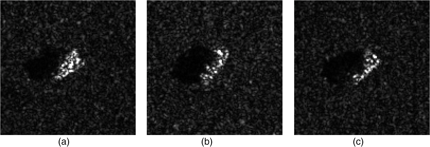
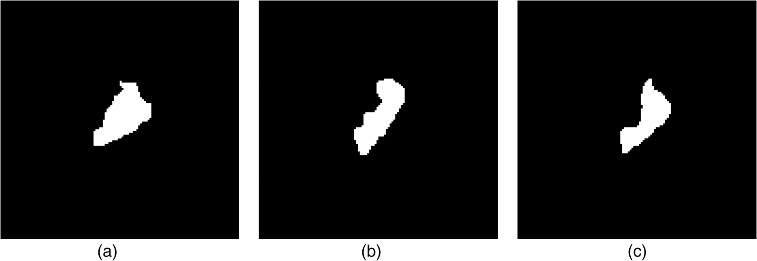
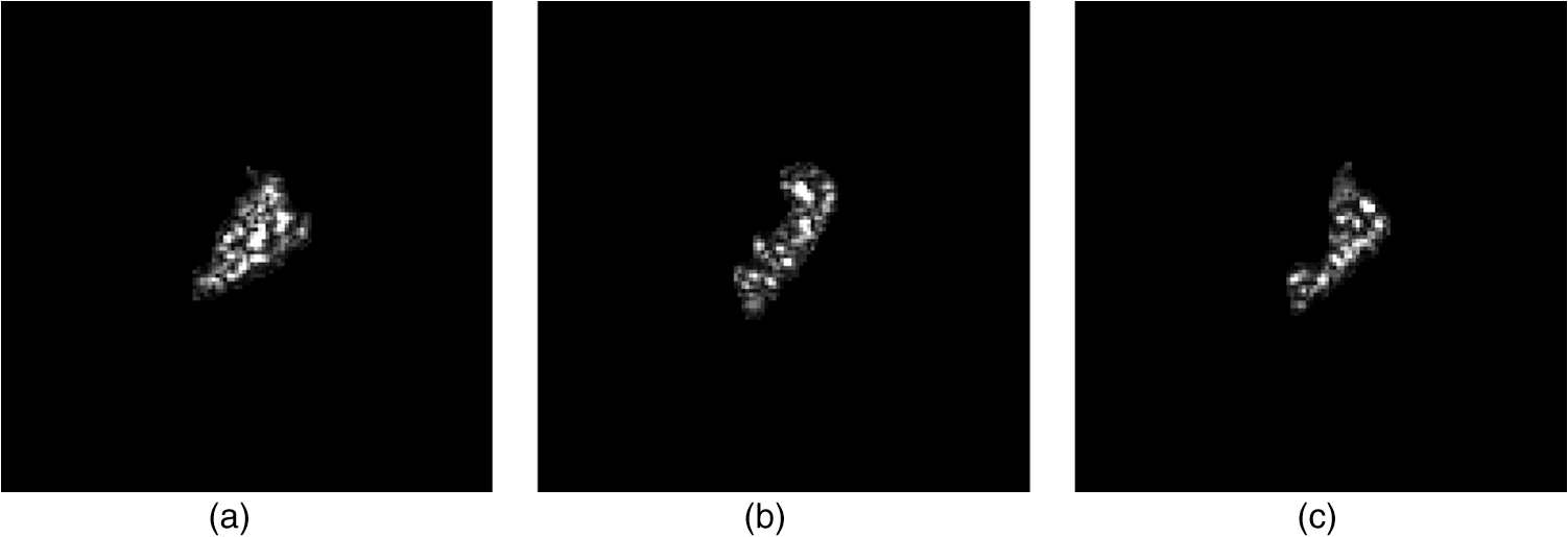
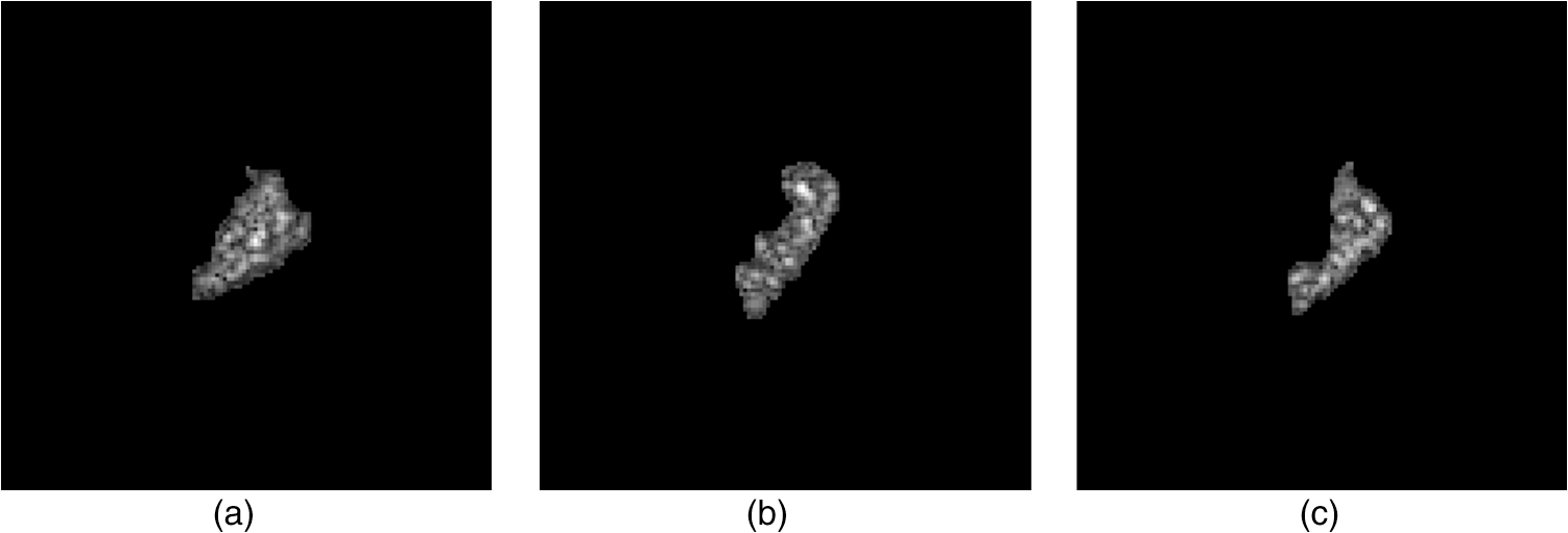
The optical images and the corresponding SAR images of the three targets in the MSTAR dataset are shown in Figs. 4 and 5. In Fig. 6, it is shown that the binary mask matrices of the targets are obtained after two-parameter CFAR and geometric clustering conducted in the SAR images. Figure 7 indicates that the target areas of SAR images are extracted, and the image registration centered on the centroid is operated. The gray enhancement and energy normalization preprocessing are executed as shown in Fig. 8.

Fig. 4

Optical images for (a) T72, (b) BTR70, and (a) BMP2 in the MSTAR database.

Fig. 5

Corresponding SAR images of three targets.

Fig. 6

Corresponding binary mask matrices of three targets.

Fig. 7

Target areas of corresponding SAR images.

Fig. 8

Preprocessed SAR images of three targets.

The AT&T face database²⁵ contains images from 40 individuals, each providing 10 different images. For some subjects, the images were taken at different times, varying the lighting, facial expressions, and facial details. All images are grayscale. For each individual, four images are randomly selected for training, and the rest are used for testing. Thus, we get 160 training samples and 240 testing samples for this experiment.

The experiment includes four parts. The theoretical approach of the proposed algorithm will be validated using the SAR image dataset in part 1. In part 2, we compare our algorithm with five other methods (PCA, LDA, KPCA, KLDA, and LDE) to evaluate the recognition performance for SAR images. We also illustrate the classification results by a two-dimensional data visualization to evaluate the performance of NVPDE. In part 3, we evaluate and discuss the influences of the relevant neighbor parameters variation for the proposed algorithm in SAR ATR. The recognition results for the face image database are demonstrated in part 4.

3.1.

Part 1

3.1.1.

Experimental steps

Because of the local Euclidean principle in manifold,⁹ samples and virtual points have a nearly linear distribution in the neighborhoods. Therefore, we utilize the scatter²⁶ to measure the spatial relationships among the data points in their neighborhoods statistically.

1. We employ the SAR image training dataset as the experiment samples in part 1. We calculate the neighborhood virtual point ${p_{i} \in R^{n}, i = 1, 2, \dots, N}$ from each neighborhood $N_{k_{1}}^{+} (x_{i})$ and compute the neighborhood scatters $ξ = [ξ_{1}, ξ_{2}, \dots, ξ_{N}] \in R^{1 \times N}$ in each $N_{k_{1}}^{+} (x_{i})$ to measure the spatial relationships between the samples and their respective neighborhood virtual points statistically, where $ξ_{i} = \frac{1}{k_{1} + 1} \sum_{x_{j} \in N_{k_{1}}^{+} (x_{i}) or i = j} {(x_{j} - p_{i})}^{T} (x_{j} - p_{i})$ , $i = 1, 2, \dots, N$ , and $N = 698$ .
2. We find the embedding $V \in R^{n \times n}$ by the NVPDE algorithm. We compute the neighborhood scatters $ξ^{'} = [ξ_{1}^{'}, ξ_{2}^{'}, \dots, ξ_{N}^{'}] \in R^{1 \times N}$ to measure the spatial relationships between the embedded samples and their respective embedded neighborhood virtual points, where $ξ_{i}^{'} = \frac{1}{k_{1} + 1} \sum_{x_{j} \in N_{k_{1}}^{+} (x_{i}) or i = j} {(V^{T} x_{j} - V^{T} p_{i})}^{T} (V^{T} x_{j} - V^{T} p_{i})$ , $i = 1, 2, \dots, N$ . We then calculate $Δ ξ = ξ - ξ^{'} = [Δ ξ_{1}, Δ ξ_{2}, \dots, Δ ξ_{N}] \in R^{1 \times N}$ to measure the neighborhood scatter variations within each sample’s neighborhood. According to the vector $Δ ξ$ and the class information, the neighborhood scatter variation stem plot of three class targets is shown in Fig. 9.
3. We follow the same routine, calculating the scatter variations $Δ ψ = ψ - ψ^{'} = [Δ ψ_{1}, Δ ψ_{2}, \dots, Δ ψ_{N}] \in R^{1 \times N}$ for each virtual point’s within-class neighborhood, where $Δ ψ_{i} = ψ_{i} - ψ_{i}^{'}$ , and the virtual point’s within-class neighborhood scatter before embedding $ψ_{i} = \frac{1}{k_{2}} \sum_{p_{j} \in N_{k_{2}}^{+} (p_{i})} {(p_{j} - p_{i})}^{T} (p_{j} - p_{i})$ and the virtual point’s within-class neighborhood scatter after embedding $ψ_{i}^{'} = \frac{1}{k_{2}} \sum_{p_{j} \in N_{k_{2}}^{+} (p_{i})} {(V^{T} p_{j} - V^{T} p_{i})}^{T} (V^{T} p_{j} - V^{T} p_{i})$ , $i = 1, 2, \dots, N$ . According to the vector $Δ ψ_{i}$ and the class information, the virtual points’ within-class neighborhood scatter variation stem plot of three class targets is shown in Fig. 10.
4. We calculate the scatter variations $Δ η = η - η^{'} = [Δ η_{1}, Δ η_{2}, \dots, Δ η_{N}] \in R^{1 \times N}$ for each virtual point’s between-class neighborhood, where $Δ η_{i} = η_{i} - η_{i}^{'}$ , and the virtual point’s between-class neighborhood scatter before embedding $η_{i} = \frac{1}{k_{3}} \sum_{p_{j} \in N_{k_{3}}^{-} (p_{i})} {(p_{j} - p_{i})}^{T} (p_{j} - p_{i})$ and the virtual point’s between-class neighborhood scatter after embedding $η_{i}^{'} = \frac{1}{k_{3}} \sum_{p_{j} \in N_{k_{3}}^{-} (p_{i})} {(V^{T} p_{j} - V^{T} p_{i})}^{T} (V^{T} p_{j} - V^{T} p_{i})$ , $i = 1, 2, \dots, N$ . According to the vector $Δ η_{i}$ and the class information, the virtual points’ between-class neighborhood scatter variation stem plot of three class targets is shown in Fig. 11.

Fig. 9

Samples’ within-neighborhood scatter variations after being embedded.

Fig. 10

Virtual points’ within-class neighborhood scatter variations after being embedded.

Fig. 11

Virtual points’ between-class neighborhood scatter variations after being embedded.

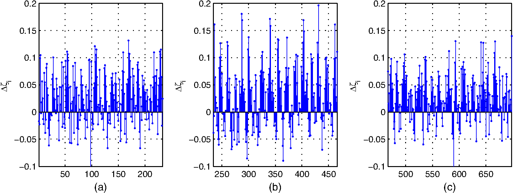
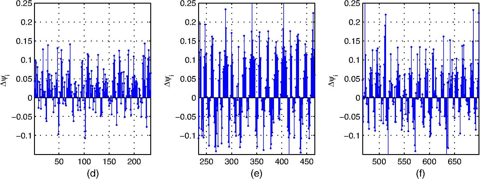
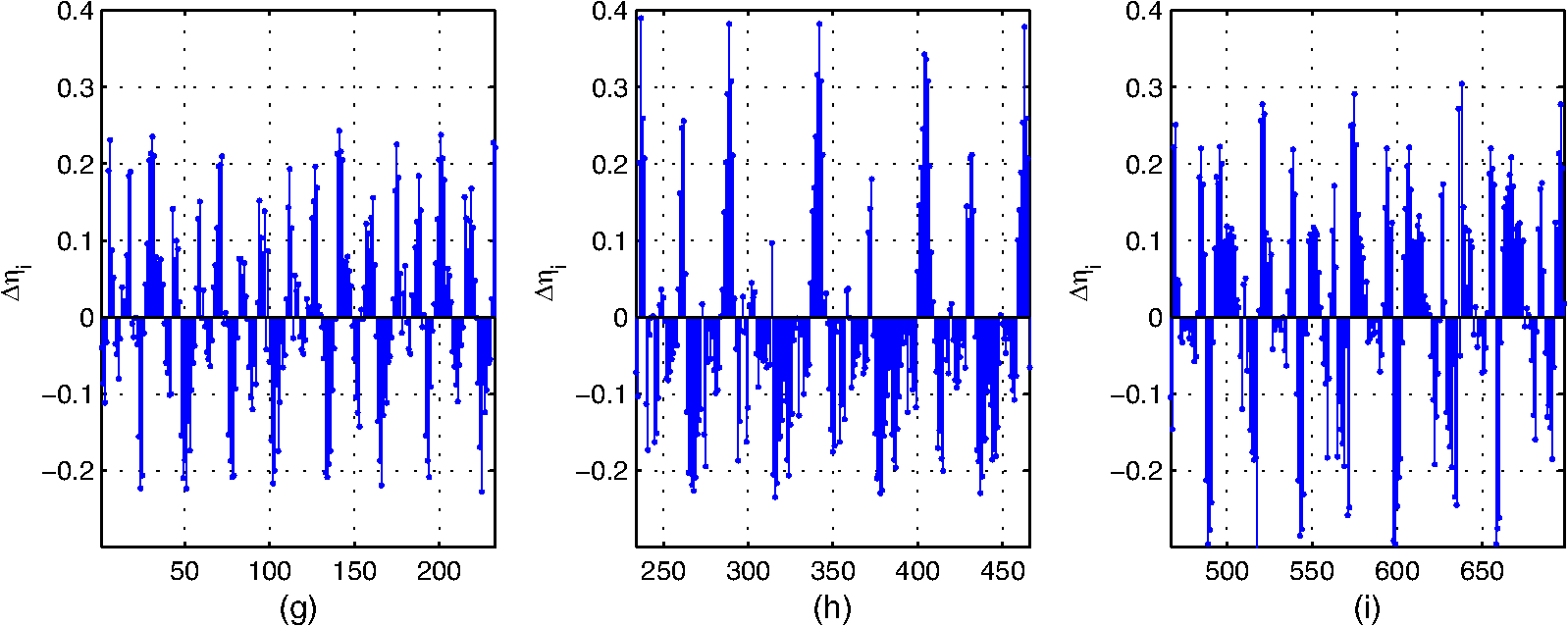
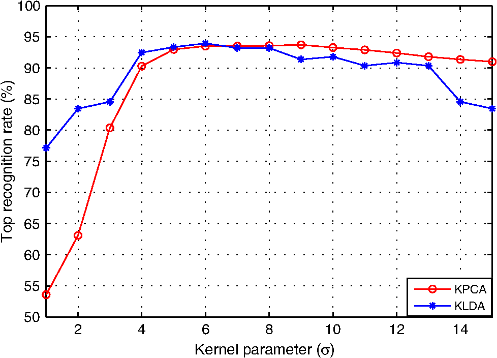
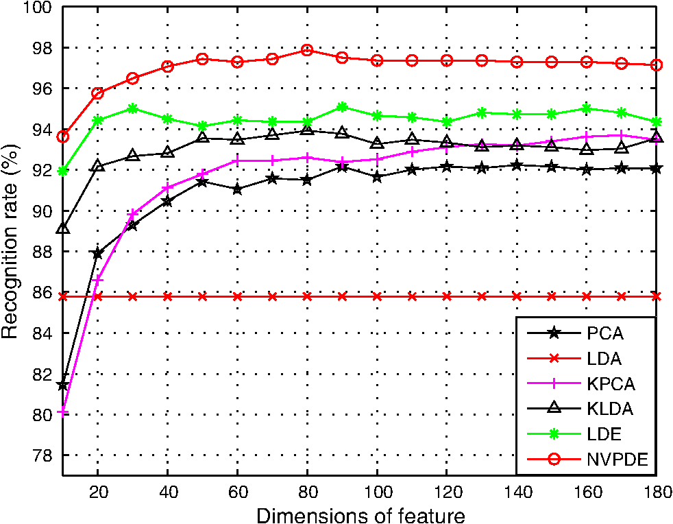
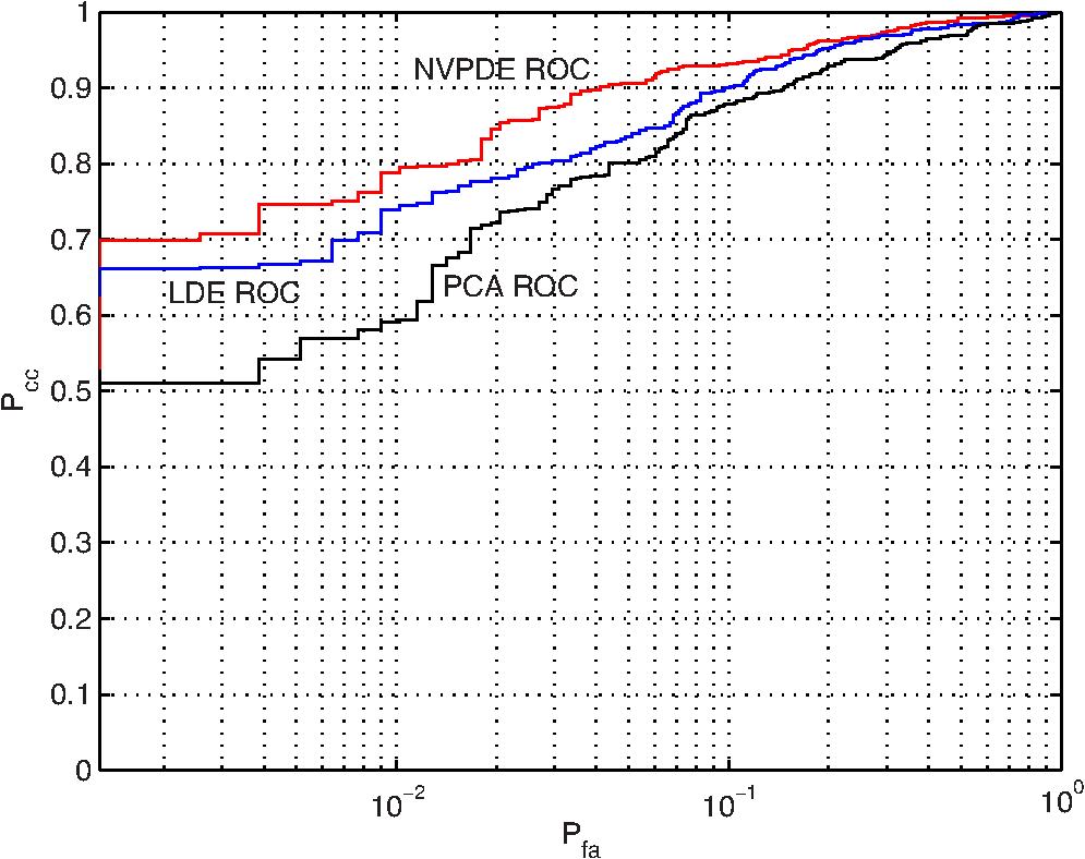
3.1.2.

Experimental results and discussions

We make some statistics according to the elements of $Δ ξ$ , $Δ ψ$ , and $Δ η$ . The proportion corresponding to the condition $Δ ξ_{i} > 0$ is 71.06%. The proportion corresponding to the condition $Δ ψ_{i} > 0$ is 61.32%, and the proportion corresponding to the condition $Δ η_{i} < 0$ is 55.59%.

According to Figs. 9 and 10 and the statistical results, it can be seen that most of the samples’ within-neighborhood scatter variations and the virtual points’ within-class neighborhood scatter variations are positive. This indicates that the samples move toward their neighborhood virtual points, and the virtual points in the same class get together by the embedding of the proposed method.

From Fig. 11 and the statistical results, it can be seen that more than half of the virtual points’ between-class neighborhood scatter variations are negative. This demonstrates that the NVPDE algorithm can keep the virtual points from different classes far away from each other in the low-dimensional space effectively.

3.2.

Part 2

3.2.1.

Experimental steps

In this experiment, PCA, LDA, KPCA, KLDA, LDE, and NVPDE are utilized to extract features of the experimental SAR image dataset. The value of neighbor parameters are $k_{1} = 10$ and $k_{2} = 20$ in LDE and $k_{1} = 18$ , $k_{2} = 20$ , and $k_{3} = 85$ in NVPDE. The nearest neighbor classifier²⁷ (NNC) is utilized for the final classification.

The kernel function of KPCA and KLDA is the Gaussian kernel $k (x_{i}, x_{j}) = \exp (- ‖ x_{i} - x_{j} ‖^{2} / σ)$ . As mentioned above, the recognition performance of the kernel method depends on the kernel settings, and the selection of the kernel settings is empirical in practice.

We change the kernel parameter gradually and get the corresponding top recognition rates. Then we evaluate the best kernel parameter.

Figure 12 shows that plots of top recognition rate versus the different values of kernel parameters using KPCA and KLDA. From this, we can see that the kernel parameters $σ = 9$ for KPCA and $σ = 6$ for KLDA are the best selections.

Fig. 12

Top recognition rate versus the different kernel parameters using KPCA and KLDA.

3.2.2.

Experimental results and discussions

Figure 13 shows plots of recognition rate versus dimensions of the feature vectors by PCA, LDA, KPCA, KLDA, LDE, and NVPDE. The maximal feature dimension based on LDA is less than the number of class $c$ .²⁸ Therefore, the recognition rate of LDA is the performance with two feature dimensions.

Fig. 13

Recognition performance of various algorithms in SAR images.

From Fig. 13, we can see that PCA and LDA have relatively low recognition rates. For the high-dimensional SAR image dataset, the manifold structure corresponds more to spatial distribution. However, the classical linear feature extraction methods, such as PCA and LDA, are all based on the global linear structure of a dataset. This limits the recognition performance of those two methods.

Figure 13 demonstrates that the recognition rates of KPCA and KLDA are similar but are significantly improved over PCA and LDA. LDE performs better than KPCA and KLDA. The NVPDE algorithm performs far better than the other methods.

The linearly inseparable problem can be transformed into a linearly separable one in a higher-dimensional space by kernel tricks, so that the linearly inseparable problem can be solved by KPCA and KLDA to some extent. However, the recognition performance depends on the selection of kernel functions, which is the main drawback of kernel tricks.

Based on manifold learning theory, LDE incorporates the class relations of samples, which can discover the low-dimensional essential structure from a high-dimensional SAR image dataset. However, this method is based only on establishing relations between samples; it ignores the spatial relationships between neighborhoods, which will restrict the recognition performance.

By introducing the neighborhood virtual point into every sample’s neighborhood in the NVPDE algorithm, the relations between the samples and their neighborhood virtual point are taken into account, and the spatial relationships of the neighborhood virtual points are established, by which the relations between neighborhoods are formed indirectly. Therefore, the algorithm is able to find out more discriminating information from the neighborhoods, and the recognition performance is far superior to LDE.

In order to evaluate the classification performance of the proposed feature extraction method systematically, we investigate the ROC of the proposed method,²⁹ and two typical feature extraction methods (PCA and LDE) were conducted for a comparison. Figure 14 shows the ROC of three feature extraction methods using NNC, and the false alarm probability axis is logarithmic.

Fig. 14

ROC comparison of the different feature extraction methods.

From Fig. 14, it can be seen that:

1. LDE and the NVPDE algorithm have a relatively high correct classification probability $(P_{cc})$ and a relatively low false alarm probability $(P_{fa})$ . Therefore, these two methods have considerable classification results.
2. NVPDE can achieve a higher correct classification probability and a lower false alarm probability than the other two methods.
3. The area under the ROC curve of the NVPDE algorithm is larger than that of PCA and LDE. This shows that the proposed algorithm has a better recognition performance than the other methods.

The top recognition rate and the corresponding dimensions by various algorithms are shown in Table 2, and we can see that our proposed algorithm outperforms the other methods.

Table 2

Best recognition performance by various algorithms.

Method	Top recognition (%)	Feature dimension
PCA	92.23	140
LDA	85.79	2
KPCA	93.70	170
KLDA	93.92	80
LDE	95.10	90
NVPDE	97.88	80

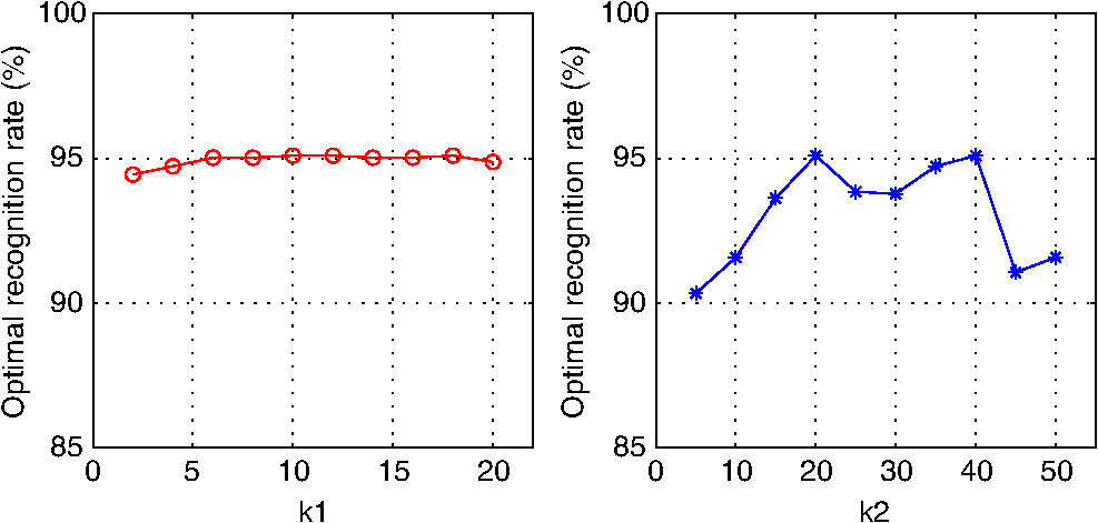
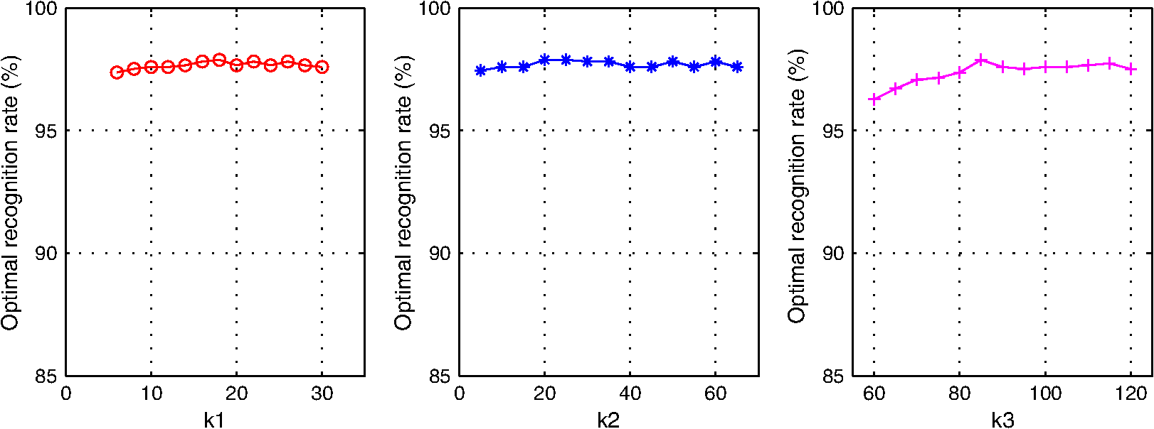
The training samples of the SAR images are embedded into two-dimensional Euclidean space by NVPDE, LDE, and PCA to illustrate the classification results with a 2-D data visualization example.

Figure 15 shows the distributions of three class samples after being embedded in two-dimensional Euclidean space by NVPDE, LDE, and PCA. The plus symbol represents the first-class samples in the embedding space, while the $o$ represents the second-class samples, and the asterisk represents the third-class samples.

Fig. 15

Distributions of three class samples after being embedded in two-dimensional Euclidean space by (a) NVPDE, (b) LDE, and (c) PCA.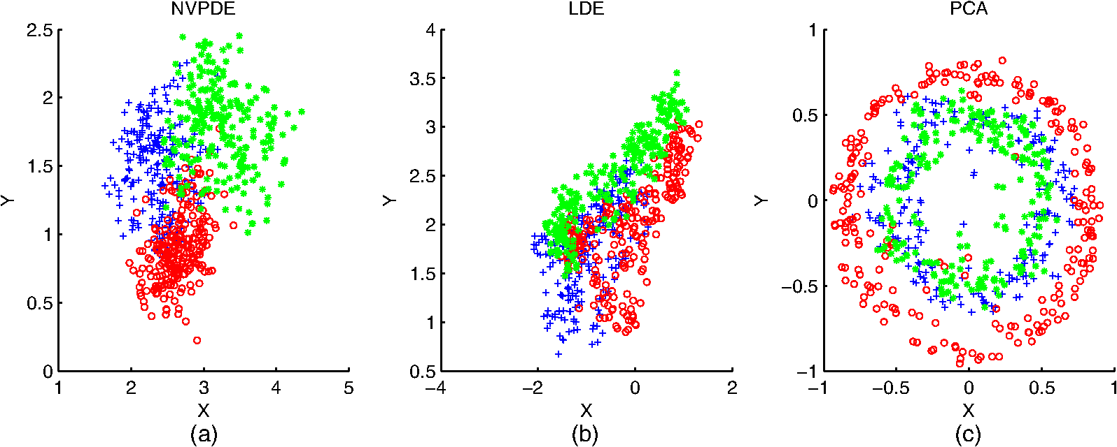

The experimental results show that samples in the same class do not get evidently close in the embedding space by PCA. After being embedded by LDE, the samples with the same class label get close to some extent, but most samples from different classes overlap with each other, which will restrict the recognition rate. By introducing the neighborhood virtual point in NVPDE, the relationships between neighborhoods are established indirectly, and more discriminating information can be found out. Hence the samples with the same class label get close, and samples from different classes separate from each other in the embedding space, as shown in Fig. 15.

3.3.

Part 3

3.3.1.

Experimental steps

In this part, LDE and NVPDE will be utilized to extract features of the experimental dataset with various neighbor parameter values. The aim is to evaluate the stability of the proposed algorithm. We set $k_{1} = 10$ and $k_{2} = 20$ in LDE and $k_{1} = 18$ , $k_{2} = 20$ , and $k_{3} = 85$ in NVPDE as the benchmark parameter settings. We then change one of the neighbor parameters gradually while keeping other parameters constant, and we record the corresponding top recognition rates of the two feature extraction methods.

3.3.2.

Experimental results and discussions

Figures 16 and 17 show the plots of top recognition rates versus the different values of neighbor parameters using LDE and NVPDE. From these figures, we can see that:

1. The variation of the within-class neighboring parameter $k_{1}$ has a tiny effect on the recognition performance in LDE, while the between-class neighboring parameter $k_{2}$ impacts the recognition performance significantly.
2. The selections of $k_{1}$ and $k_{2}$ influence the recognition results of NVPDE slightly, and $k_{3}$ has an effect on the recognition performance to some extent, but it is much smaller than $k_{2}$ in LDE.

Fig. 16

Top recognition rate versus different neighbor parameters using LDE.

Fig. 17

Top recognition rate versus different neighbor parameters using NVPDE.

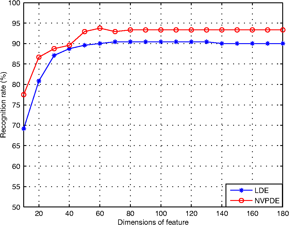
Because the curvature and density may vary over the manifold,³⁰ as an open problem,³¹ the values of neighbor parameters are likely to influence the result of recognition as in LDE.

In the NVPDE algorithm, the neighborhood virtual point of each sample is computed. In this way, the mean of each neighborhood is calculated, which is able to smooth the neighborhood of each sample and weaken the influence of neighbor parameters on recognition performance. Therefore, the selection of neighbor parameters has a very small effect on the classification results of our proposed method.

3.4.

Part 4

3.4.1.

Experimental steps

In this part, we take advantage of the AT&T face database to examine the applicability of the proposed method in optical image recognition. LDE and NVPDE are utilized to extract features of the experimental AT&T dataset. The values of the neighbor parameters are $k_{1} = 3$ and $k_{2} = 30$ in LDE and $k_{1} = 3$ , $k_{2} = 3$ , and $k_{3} = 30$ in NVPDE. NNC is used for the final classification.

3.4.2.

Experimental results and discussions

Figure 18 shows plots of recognition rates versus the dimensions of the feature vectors by LDE and NVPDE. In Fig. 18, the best recognition rate is 90.42% with the corresponding feature dimension 70 for LDE, while the top recognition rate can get to 93.75% with the corresponding feature dimension 60 in NVPDE. This means that the recognition performance of the proposed method outperforms LDE for the AT&T face database. Therefore, the experimental results indicate that the NVPDE method can achieve a satisfactory recognition performance in optical image recognition, as well.

Fig. 18

Recognition performance of LDE and NVPDE in face images.

4. Conclusion

For the issue of feature extraction from high-dimensional SAR images, it is important to establish relationships between samples’ neighborhoods, which will uncover much more discriminating information. In this paper, a new approach to feature extraction was proposed, in which the neighborhood virtual points are employed and the relationships between neighborhoods are taken into account sufficiently. Through this method, classification is better conducted in feature space, and the recognition performance is improved. The experimental results based on the MSTAR dataset demonstrate the effectiveness of our method.

Acknowledgments

This research was supported by the National Natural Science Foundation of China (No. 61201272).

References

1.

M. TurkA. Pentland, “Eigenfaces for recognition,” J. Cognit. Neurosci., 3 (1), 71 –86 (1991). http://dx.doi.org/10.1162/jocn.1991.3.1.71 JCONEO Google Scholar

2.

P. N. Belhumeuret al., “Eigenfaces vs. Fisherfaces: recognition using class specific linear projection,” IEEE Trans. Pattern Anal. Mach. Intell., 19 (7), 711 –720 (1997). http://dx.doi.org/10.1109/34.598228 ITPIDJ 0162-8828 Google Scholar

3.

A. K. Mishra, “Validation of PCA and LDA for SAR ATR,” in TENCON 2008—2008 IEEE Region 10 Conf., 1 –6 (2008). Google Scholar

4.

Q. ZhaoJ. C. Principe, “Support vector machines for SAR automatic target recognition,” IEEE Trans. Aerosp. Electron. Syst., 37 (2), 643 –654 (2001). http://dx.doi.org/10.1109/7.937475 IEARAX 0018-9251 Google Scholar

5.

B. Scholkopfet al., “Kernel principal component analysis,” Advances in Kernel Methods-Support Vector Learning, 327 –352 MIT Press, Cambridge, Massachusetts (1999). Google Scholar

6.

S. Mikaet al., “Fisher discriminant analysis with kernels,” in Proc. 1999 IEEE Signal Processing Society Workshop, 41 –48 (1999). Google Scholar

7.

H. S. Seunget al., “The manifold ways of perception,” Science, 290 (5500), 2268 –2269 (2000). http://dx.doi.org/10.1126/science.290.5500.2268 SCIEAS 0036-8075 Google Scholar

8.

J. B. Tenenbaumet al., “A global geometric framework for nonlinear dimensionality reduction,” Science, 290 (5500), 2319 –2323 (2000). http://dx.doi.org/10.1126/science.290.5500.2319 SCIEAS 0036-8075 Google Scholar

9.

S. T. RoweisL. K. Saul, “Nonlinear dimensionality reduction by locally linear embedding,” Science, 290 (5500), 2323 –2326 (2000). http://dx.doi.org/10.1126/science.290.5500.2323 SCIEAS 0036-8075 Google Scholar

10.

M. BelkinP. Niyogi, “Laplacian eigenmaps and spectral techniques for embedding and clustering,” in Proc. Adv. Neural Inform. Process. Syst., 585 –592 (2002). Google Scholar

11.

X. HeP. Niyogi, “Locality preserving projections,” in Proc. 16th Conf. Neural Information Processing Systems, 103 (2003). Google Scholar

12.

X. Heet al., “Neighborhood preserving embedding,” in Proc. 11th International Conf. Computer Vision, 1208 –1213 (2005). Google Scholar

13.

E. KokiopoulouY. Saad, “Orthogonal neighborhood preserving projections: A projection-based dimensionality reduction technique,” IEEE Trans. Pattern Anal. Mach. Intell., 29 (12), 2143 –2156 (2007). http://dx.doi.org/10.1109/TPAMI.2007.1131 ITPIDJ 0162-8828 Google Scholar

14.

H. Caiet al., “ISAR target recognition based on manifold learning,” in Proc. IET International Radar Conf., 1 –4 (2009). Google Scholar

15.

B. Wanget al., “A feature extraction method for synthetic aperture radar (SAR) automatic target recognition based on maximum interclass distance,” Sci. China Tech. Sci., 54 (9), 2520 –2524 (2011). http://dx.doi.org/10.1007/s11431-011-4430-0 SCTSBO 1674-7321 Google Scholar

16.

H. T. Chenet al., “Local discriminant embedding and its variants,” in IEEE Computer Society Conf. Computer Vision and Pattern Recognition, 846 –853 (2005). Google Scholar

17.

M. Bryant, “Target signature manifold methods applied to MSTAR dataset: preliminary results,” Proc. SPIE, 4382 389 –394 (2001). http://dx.doi.org/10.1117/12.438232 PSISDG 0277-786X Google Scholar

18.

V. Venkataramanet al., “Automated target tracking and recognition using coupled view and identity manifolds for shape representation,” EURASIP J. Adv. Sig. Proc., 2011 (1), 1 –17 (2011). http://dx.doi.org/10.1186/1687-6180-2011-124 Google Scholar

19.

R. A. Fisher, “The use of multiple measurements in taxonomic problems,” Ann. Human Gen., 7 (2), 179 –188 (1936). http://dx.doi.org/10.1111/j.1469-1809.1936.tb02137.x ANHGAA 0003-4800 Google Scholar

20.

T. Rosset al., “Standard SAR ATR evaluation experiments using the MSTAR public release dataset,” Proc. SPIE, 3370 566 –573 (1998). http://dx.doi.org/10.1117/12.321859 PSISDG 0277-786X Google Scholar

21.

T. Wang, “SAR automatic target recognition method research based on manifold learning,” http://d.g.wanfangdata.com.cn/Thesis_Y1707370.aspx Google Scholar

22.

L. M. Novaket al., “Performance of a high-resolution polarimetric SAR automatic target recognition system,” Lincoln Lab. J., 6 (1), 11 –24 (1993). Google Scholar

23.

T. Wanget al., “SAR ATR based on generalized principal component analysis integrating class information,” in Proc. IET International Radar Conf., 1 –4 (2009). Google Scholar

24.

R. C. GonzalezR. E. Woods, Digital Image Processing, 80 –84 Prentice Hall, New Jersey (2008). Google Scholar

25.

, “The AT&T Database of Faces,” (2002) http://www.cl.cam.ac.uk/research/dtg/attarchive/facedatabase.html Google Scholar

26.

S. TheodoridisK. Koutroumbas, Pattern Recognition, 280 –299 Elsevier Inc., Amsterdam, Holland (2011). Google Scholar

27.

T. Cover, “Estimation by the nearest neighbor rule,” IEEE Trans. Inform. Theory, 14 (1), 50 –55 (1968). http://dx.doi.org/10.1109/TIT.1968.1054098 IETTAW 0018-9448 Google Scholar

28.

A. M. MartinezA. C. Kak, “PCA versus LDA,” IEEE Trans. Pattern Anal. Mach. Intell., 23 (2), 228 –233 (2001). http://dx.doi.org/10.1109/34.908974 ITPIDJ 0162-8828 Google Scholar

29.

A. K. Mishraet al., “Automatic target recognition,” Encyclopedia of Aerospace Engineering, John Wiley & Sons Ltd., Hoboken, New Jersey (2010). Google Scholar

30.

N. MekuzJ. Tsotsos, “Parameterless ISOMAP with adaptive neighborhood selection,” Pattern Recognition, 364 –373 Springer, Berlin, Heidelberg (2006). Google Scholar

31.

Y. Shuichenget al., “Graph embedding and extensions: A general framework for dimensionality reduction,” IEEE Trans. Pattern Anal. Mach. Intell., 29 (1), 40 –51 (2007). http://dx.doi.org/10.1109/TPAMI.2007.250598 ITPIDJ 0162-8828 Google Scholar

Biography

Jifang Pei received a BS from the College of Information Engineering at Xiangtan University, Hunan, China, in 2010. He is an IEEE student member and is working toward an MSc degree at the University of Electronic Science and Technology of China (UESTC), Chengdu. His research interests include SAR automatic target recognition and digital image processing.

Yulin Huang received his BS and PhD degrees in electronic engineering from the University of Electronic Science and Technology of China, Chengdu, in 2002 and 2008, respectively. He is an IEEE member and an associate professor at UESTC. His ﬁelds of interest include radar signal processing and SAR automatic target recognition.

Xian Liu received a BS degree from the Institute of Information Science and Engineering at Hebei University of Science and Technology, China, in 2009. She is an IEEE student member and is working toward a PhD degree at UESTC. Her fields of interest include SAR automatic target recognition.

Jianyu Yang received a BS degree from the National University of Defense Technology, Changsha, China, in 1984, and MS and PhD degrees from UESTC in 1987 and 1991, respectively. All his degrees are in electronic engineering. He is a professor at UESTC and a senior editor for the Chinese Journal of Radio Science. He is a member of IEEE and the Institution of Engineering and Technology and a senior member of the Chinese Institute of Electronics.

CC BY: © The Authors. Published by SPIE under a Creative Commons Attribution 4.0 Unported License. Distribution or reproduction of this work in whole or in part requires full attribution of the original publication, including its DOI.

Citation Download Citation

Jifang Pei, Yulin Huang, Xian Liu, and Jianyu Yang "Neighborhood virtual points discriminant embedding for synthetic aperture radar automatic target recognition," Optical Engineering 52(3), 036201 (7 March 2013). https://doi.org/10.1117/1.OE.52.3.036201

Published: 7 March 2013

Access the abstract

JOURNAL ARTICLE
12 PAGES

DOWNLOAD PAPER SAVE TO MY LIBRARY

GET CITATION

CITATIONS

Cited by 5 scholarly publications.

Explore citations on Lens.org

KEYWORDS

Synthetic aperture radar

Feature extraction

Principal component analysis

Detection and tracking algorithms

Automatic target recognition

Optical engineering

Databases

1.

Introduction

2.