Spatial and interlayer hybrid intra-prediction for H.264/SVC video

Chun-Su Park

doi:10.1117/1.OE.52.7.071503

4 March 2013 Spatial and interlayer hybrid intra-prediction for H.264/SVC video

Chun-Su Park

Author Affiliations +

Optical Engineering, Vol. 52, Issue 7, 071503 (March 2013). https://doi.org/10.1117/1.OE.52.7.071503

Abstract

A spatial and interlayer hybrid intra-prediction (SILHIP) scheme is proposed in this work to improve the coding efficiency of the scalable video coding (SVC) standard. The SVC standard adopts a line-by-line intra-prediction that predicts the texture information of a block by exploiting the spatial correlation between adjacent blocks. However, the accuracy of the line-by-line intra-prediction deteriorates when a target block lies in the edge region. The proposed SILHIP scheme adaptively predicts a target block by exploiting both the spatial correlation and the interlayer correlation between the base layer and the enhancement layer. To implement the SILHIP scheme, we partition a macroblock into two regions based on the edge map and allow different types of prediction schemes to be used in different regions. It is shown by experimental results that the proposed SILHIP scheme outperforms the conventional one consistently.

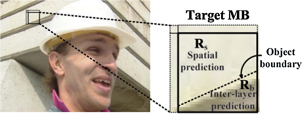
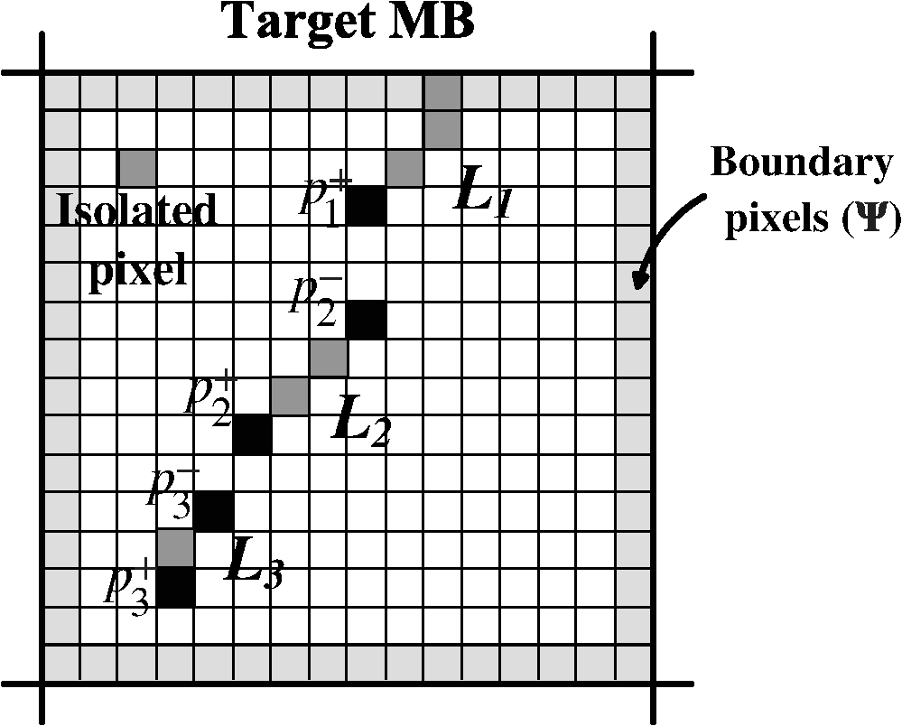
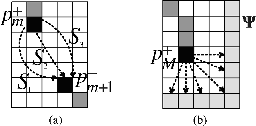
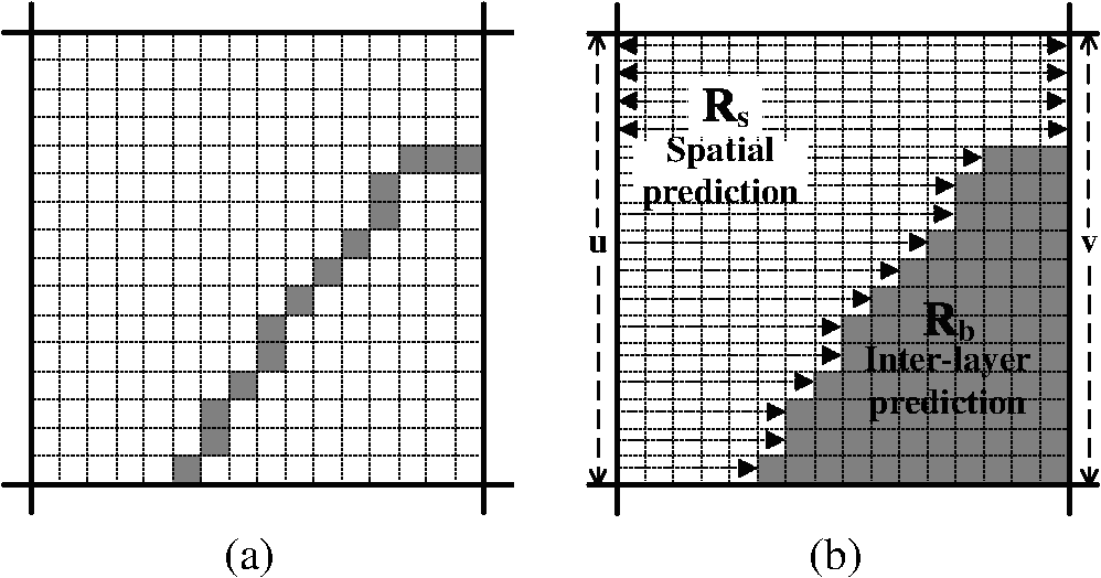
1. Introduction

Due to increased demand in video broadcasting/streaming over heterogeneous networks, video content has to be broadcasted/streamed to multiple users with different display and networking capabilities. The scalable extension of the H.264/AVC standard, called scalable video coding (SVC), provides a state-of-the-art solution to this problem. In the SVC scenario, the video signal is split into several layers, and a receiver may decode a part of the bitstream due to its resource constraint.¹^–³

Intra-prediction is an efficient method to reduce spatial redundancy in coded video data.⁴ Both H.264/AVC and SVC adopt the line-by-line intra-prediction scheme.⁵ The prediction signal is constructed by extrapolating pixels of neighboring blocks that precede the target block in the coding order. The intra-prediction is applied to $4 \times 4$ , $8 \times 8$ , or $16 \times 16$ blocks for the luma component while it is applied only to the macroblock (MB) for the chroma components. Since the base layer (BL) of SVC is compatible with the H.264/AVC specifications, the intra-prediction scheme of H.264/AVC is utilized to encode frames of the BL.

In SVC, a frame of the enhancement layer (EL) can be predicted using frames of a lower layer as well as the current layer. The SVC standard adopts several interlayer prediction schemes to improve the EL coding performance. Among them, the interlayer intra-prediction (ILIP) scheme introduces an additional coding mode, denoted by I_BL, to encode the EL MB of an intra frame. When an EL MB is encoded with mode I_BL, its prediction is obtained by upsampling the BL block at the co-located position.²^,⁶ It has been shown that I_BL improves the coding efficiency of the EL significantly.

Here we attempt to improve the performance of the existing intra-prediction by developing a spatial and interlayer hybrid intra-prediction (SILHIP) scheme. The proposed SILHIP scheme exploits the spatial correlation as well as the interlayer correlation between the BL and the EL adaptively. To implement the SILHIP scheme, we partition an MB into two regions with an edge map and allow different types of prediction schemes to be used in different regions. It is shown by experimental results that the proposed scheme can reduce the bit rate by 1.67 to 8.22%.

The rest of this paper is organized as follows. Related previous work is reviewed, and our basic idea is presented in Sec. 2. The edge map construction is examined in Sec. 3. The SILHIP scheme is described in Sec. 4. Experimental results are shown in Sec. 5, and concluding remarks are given in Sec. 6.

2. Review of Previous Work and Basic Idea

Generally speaking, the farther a pixel is away from the block boundary of a target MB, the less accurate the prediction is, which results in coding efficiency loss.⁴ Moreover, the prediction accuracy degrades significantly if a target block is located in the edge region of an object. Although the line-by-line intra-prediction tries to take the edge effect into account by specifying a couple of edge orientations, the number of the preset edge orientations is limited. Besides, an object may have a curved boundary. Several techniques⁷^,⁸ have been proposed to improve the intra-prediction performance of H.264/AVC by exploiting local features of a frame. Although these techniques can be potentially applied to each layer of SVC separately, their application may not produce satisfactory results since the interlayer correlation was not exploited.⁷^,⁸

It was pointed out by Wang et al.⁹ that, when encoding blocks in slice boundaries, pixels of their neighboring blocks are not available. They proposed a new intra-coding scheme to encode an intra-frame of the EL to overcome this difficulty. They use pixels of the BL to improve prediction accuracy for the EL MB. However, since their method does not consider local features of a frame, the performance gain is limited. Liu et al.¹⁰ introduced a new method that improves the intra-prediction of the EL. This method constructs the prediction signal of the EL by adaptively allowing interlayer prediction for each $4 \times 4$ block. More recently, Park et al.¹¹ proposed an improved interlayer intra-prediction (ILIP) algorithm based on the displacement vector (DV). By observing a phase shift between the BL and the EL, they proposed to signal the DV to indicate the phase difference. However, the intra-prediction scheme of SVC remains the same.¹¹

The basic idea of the proposed SILHIP scheme is illustrated in Fig. 1 by an example. Due to the existence of the object boundary, there are two regions denoted by $R_{s}$ and $R_{b}$ in the target MB as given in Fig. 1. The left and the top boundaries of region $R_{s}$ are surrounded by pixels that have already been reconstructed. It seems natural to encode region $R_{s}$ by exploiting the spatial correlation. In contrast, we have little information about region $R_{b}$ from the same layer and should exploit the interlayer correlation. For this purpose, we need to determine whether there exists an object boundary for each MB. This can be achieved by edge detection and connection that will be detailed in Sec. 3. Then, we will discuss how to choose the spatial line-prediction or the interlayer prediction dynamically.

Fig. 1

Basic idea of the proposed SILHIP scheme.

3. Edge Map Construction

Detecting salient boundaries in an image involves two steps: edge detection and edge connection.¹² In the first step, we construct a set of segments by running an edge detector on the input image and approximating detected edges with a set of segments, which are referred to as detected edge segments. Since detected edge segments are often disconnected from one another, we need to fill in gaps between them to form a closed contour. In the second step, we connect all relevant pairs of endpoints of different detected segments. Finally, a boundary is defined as a straight or curved line that traverses a set of detected and gap-filled segments alternately. We describe these two steps in detail below.

3.1.

Edge Segment Detection

The proposed SILHIP method predicts the edge in a target EL block using the corresponding BL block. We use $B$ and $B^{u}$ to denote the target EL MB to be coded and the upsampled MB using the BL block corresponding to $B$ , respectively. In SVC, $B^{u}$ is obtained using the one-dimensional 4-tap FIR filter for the luma component and the bi-linear filter for the chroma components.² Edge detection is essentially to find a high intensity gradient in a certain region. Here we calculate the intensity gradient at each pixel for horizontal and vertical directions separately. We will discuss the process along the horizontal direction only. The same procedure can be conducted in the vertical direction too. We compute the intensity gradient in the horizontal direction as

Eq. (1)

G_{h} (x, y) = \nabla_{x} B^{u} (x, y) = B^{u} (x, y) - B^{u} (x - 1, y),

where

(x, y)

is the pixel coordinates in

B^{u}

. Then we determine the binary edge map,

E_{h}

, representing the locations of the detected edge segments as

Eq. (2)

E_{h} (x, y) = {\begin{matrix} 1, & if G_{h} (x, y) > T \\ 0, & otherwise \end{matrix},

where

T

is a threshold.

We remove isolated points that might occur due to image noise, quantization error, etc.¹³ Let $Ω$ be the set of all pixels satisfying $E_{h} (x, y) = 1$ . Then we define a pixel in $Ω$ as an isolated one if none of its eight neighbors is an element in $Ω$ . For example, the single pixel in the upper-left corner of Fig. 2 is an isolated one. After removing isolated pixels, the remaining pixels in $Ω$ can be clustered into several connected segments. In the ideal case where a single edge exists inside the target block, we can simply obtain the outermost object boundary using the detected edge information. However, if there is a complicate edge, e.g., cross edge, the target block may contain multiple edge lines. Thus we extract the line segments at the outermost object boundary by removing all pixels from $Ω$ except the outermost pixels. For example, if there are two pixels, $(x_{1}, y)$ and $(x_{2}, y)$ , satisfying $G_{h} (x_{1}, y) > T$ , $G_{h} (x_{2}, y) > T$ , and $x_{1} < x_{2}$ , the final edge map $E_{h}$ contains only $(x_{1}, y)$ , i.e., the pixel $(x_{2}, y)$ is removed from $E_{h}$ . Then, $E_{h}$ finally contains the line segments at the outermost object boundary in the target block.

Fig. 2

Graphical examples of edge segments and their endpoints.

3.2.

Edge Segment Connection

After constructing line segments, we need to fill the gaps between detected line segments to form a complete boundary between regions. Let $L = {L_{1}, L_{2}, \dots, L_{m}, \dots, L_{M}}$ be $M$ detected line segments in the target MB and $P_{m} = {p_{m}^{+}, p_{m}^{-}}$ be the set of endpoints belonging to $L_{m}$ . The endpoints of edge segments can be easily detected using the morphological filter. Figure 2 shows an example of $L_{m}$ and $P_{m}$ , where $Ψ$ is the set of pixels in the block boundary. In the example, since one of the endpoints of $L_{1}$ is belonging to $Ψ$ , $L_{1}$ has only one endpoint ( $P_{1} = {p_{1}^{+}}$ ). In case of $L_{2}$ , since it locates inside the target MB, the number of endpoints is equal to 2 ( $P_{2} = {p_{2}^{+}, p_{2}^{-}}$ ).

After constructing line segments and their endpoints, the proposed method finds gap-filling line segment between the detected line segments. In this study, we introduce a gap-filling cost (GFC) to connect the detected line segments. Basically, among all possible gap-filling line segments connecting $p_{m}^{+}$ and $p_{m + 1}^{-}$ , we find the best one that minimizes the GFC. Let $S_{i} (p_{m}^{+}, p_{m + 1}^{-})$ be the $i$ ’th line segment filling the gap between $p_{m}^{+}$ and $p_{m + 1}^{-}$ . At first, for all possible paths between $p_{m}^{+}$ and $p_{m + 1}^{-}$ , we calculate the GFCs of $S_{i}$ ’s based on the intensity gradient as

Eq. (3)

J [S_{i} (p_{m}^{+}, p_{m + 1}^{-})] = \sum_{(x, y) \in S_{i} (p_{m}^{+}, p_{m + 1}^{-})} \frac{1}{G_{h} (x, y) + 1} .

Then, among all possible

S_{i}

’s, we choose the best one

S^{*}

which has the minimum GFC as

Eq. (4)

S^{*} = \underset{\forall S_{i}}{argmin} J [S_{i} (p_{m}^{+}, p_{m + 1}^{-})] .

If there are multiple paths sharing the same minimum cost, we choose the one with the shortest two-dimensional Euclidean distance. And the two endpoints, $p_{1}^{-}$ and $p_{M}^{+}$ , if present, are connected with one of the pixels in $Ψ$ . The proposed gap-filling process is illustrated in Fig. 3. Note that, in the proposed method, even if the original object does not reach the block boundary, the proposed method finds the shortest path between the object and block boundary and then constructs the edge map as if the block reached the boundary.¹⁴^,¹⁵

Fig. 3

Illustration of the gap-filling process: (a) between $p_{m}^{+}$ and $p_{m + 1}^{-}$ , (b) between $p_{M}^{+}$ and block boundary $Ψ$ .

This gap-filling process is repeated until all endpoints in the target MB are connected. Finally, we obtain the closed binary edge map, $E_{h}^{c}$ , of the target MB, which will serve as the input to the hybrid intra-prediction process. Since we construct the edge map by considering the local feature of the image, the proposed approach is generally applicable than the traditional line-by-line intra-prediction. For example, it can handle curved boundaries. One can obtain the closed binary edge map, $E_{v}^{c}$ , for the vertical direction in a similar fashion.

Note that the proposed SILHIP adopts a relatively simple gradient-based edge-detection method. In addition, since the edge connection for an endpoint is performed only between the endpoint and the closest one of another edge segment, the complexity is not increased significantly. In the experiment, we measure the encoding-time increment due to the proposed SILHIP.

4. Proposed Hybrid Intra-Prediction

The conventional intra-prediction method is applied to $4 \times 4$ , $8 \times 8$ , or $16 \times 16$ blocks. The proposed SILHIP method can also be applied to $4 \times 4$ , $8 \times 8$ , or $16 \times 16$ blocks. For simplicity, we focus our discussion on the SILHIP method for the $16 \times 16 MB$ in this section. The other two cases can be easily generalized.

4.1.

Prediction Signal Construction

When the target block is at the edge of moving objects or on the boundary between two objects with different characteristics, the spatial correlation is not strong enough to predict the target block, leading to the degradation of the prediction accuracy. To address this issue, we divide a target MB into two regions, $R_{s}$ and $R_{b}$ , where $R_{s}$ and $R_{b}$ represent the regions to be predicted based on spatial correlation and interlayer correlation, respectively.

For the MB containing an object boundary, the connected edge segments divide the target MB into two disjoint regions. By scanning a row from left to right (or a column from top to down), we may fill the segment that goes beyond the edge point with 1’s and denote such an operation by $F (\cdot)$ . Then, using the binary edge maps, $E_{h}^{c}$ and $E_{v}^{c}$ , we have

Eq. (5)

R_{b} = F (E_{h}^{c}) \cup F (E_{v}^{c}) .

Then, the remaining pixels are assigned to

R_{s}

. After dividing the target MB into

R_{s}

and

R_{b}

, the hybrid prediction signal is constructed using the information of the BL and EL. At the decoder, the following parsing process is performed:

• If $(x, y) \in R_{s}$ , the prediction signal is obtained based on the conventional intra-prediction scheme adopted in the SVC standard. Note that, in this case, the prediction signal is constructed according to the coded intra-prediction mode.
• If $(x, y) \in R_{b}$ , the prediction signal cannot be constructed by exploiting the spatial correlation. In this case, we use the upsampled BL block $B^{u}$ as the prediction signal.

4.2.

Enhanced Horizontal and Vertical Modes in SILHIP

In many video sequences, most of the texture directions are vertical and horizontal. Thus, it was shown that the vertical and horizontal modes are dominant among all intra-prediction modes.¹⁶^,¹⁷ In order to reduce the computational complexity and improve the coding efficiency of the proposed method, we introduce an improved prediction method for the horizontal and vertical modes. We will explain the details of the proposed method only for the horizontal mode. Similarly, the prediction signal for the vertical mode can be obtained. In the horizontal mode, the prediction signal is constructed by simply copying the column immediately to the left of the target MB. Thus, in this case, we define $R_{b}$ as follows

Eq. (6)

R_{b} = F (E_{h}^{c}) .

Figure 4 shows an example of the proposed prediction signal construction process for the horizontal mode.

Fig. 4

Examples of (a) $E_{h}^{c}$ and (b) $F (E_{h}^{c})$ .

In Ref. 9, an interpolation-based intra-prediction scheme was proposed. The intra-prediction signal is constructed by using the reconstructed pixels of the lower layer. Similarly, we can improve the performance of the proposed method for the vertical and horizontal modes. Let $u$ and $v$ be the column vectors immediately to the left and right of the target MB, respectively, as shown in Fig. 4(b). When the target EL MB is encoded, all pixels of the preceding EL MB in the raster scan order have already been reconstructed. Thus, we can set $u$ to values of the previously reconstructed EL block in the left. Although we do not have the value of $v$ , we can use the upsampled BL block in the right for its prediction. Then the prediction signal for the horizontal mode can be constructed by a linear interpolation of values of $u$ and $v$ . Note that this prediction scheme is not applied to the row of the target MB, which includes any edge pixels.

5. Experimental Results

In the experiments, we used the joint scalable video model (JSVM) 9.17 reference software,¹⁸ and evaluated the performance of the proposed SILHIP method by utilizing several sequences with CIF, 4CIF, and 1080p formats. We calculated the average bitrate and the PSNR value of the EL for test video sequences consisting of 100 frames. It is observed that the coding efficiency of the proposed SILHIP method can be enhanced by adaptively adjusting threshold $T$ for edge detection in Eq. (2). Thus, we added a parameter to indicate threshold $T$ to each slice header.

We implemented the proposed SILHIP scheme by modifying the original intra-prediction scheme in the SVC standard, i.e., the original intra-prediction scheme is not used at the EL in the proposed method. Test conditions are summarized in Table 1. Tables 2 and 3 represent the simulation results, where $Δ B$ and $Δ P$ denote the average bitrate reduction and the PSNR change of the proposed SILHIP method, respectively. And, $Δ C$ indicates the increase of the encoding time for given $T$ .

Table 1

Encoder configurations.

Parameters	Value
$8 \times 8$ transform	On
Number of frames	100
Coding modes	INTRA_ $16 \times 16$ , INTRA_ $8 \times 8$ , INTRA_ $4 \times 4$ , and I_BL
Quantization	(28,22), (32,26), and (36,30)
Mode selection	Rate-distortion optimization (RDO) on
Entropy coding	Context-adaptive variable-length coding (CAVLC)

Table 2

Performance comparison of the conventional and proposed SILHIP methods for CIF and 4CIF sequences.

Sequences	$(Q_{b}, Q_{e})$	JSVM		Liu		Proposed
Sequences	$(Q_{b}, Q_{e})$	Bitrate (kbps)	PSNR (dB)	$Δ B$ (%)	$Δ P$ (dB)	$Δ B$ (%)	$Δ P$ (dB)	$Δ C$ (%)
City (CIF@30 fps)	(28,22)	3207.41	40.55	$- 0.47$	0.00	$- 2.28$	$- 0.02$	13.27
	(32,26)	2430.02	37.11	$- 0.64$	0.00	$- 3.01$	$- 0.04$	13.42
	(36,30)	1821.29	34.13	$- 1.19$	0.01	$- 4.09$	$- 0.06$	14.12
Crew (CIF@30 fps)	(28,22)	2173.06	42.06	$- 1.06$	0.01	$- 2.97$	$- 0.04$	13.35
	(32,26)	1522.23	39.22	$- 1.46$	0.01	$- 3.74$	$- 0.06$	14.14
	(36,30)	1102.87	36.66	$- 2.15$	0.02	$- 4.34$	$- 0.09$	14.70
Foreman (CIF@30 fps)	(28,22)	2420.36	41.35	$- 1.05$	0.01	$- 2.54$	$- 0.03$	11.98
	(32,26)	1613.88	38.44	$- 1.49$	0.02	$- 3.75$	$- 0.04$	14.09
	(36,30)	1128.85	35.98	$- 2.28$	0.03	$- 5.36$	$- 0.05$	13.93
Harbour (CIF@30 fps)	(28,22)	3553.91	40.33	$- 0.53$	0.00	$- 1.89$	$- 0.01$	11.88
	(32,26)	2787.05	36.75	$- 0.51$	0.00	$- 2.35$	$- 0.02$	14.17
	(36,30)	2219.52	33.62	$- 0.64$	0.00	$- 3.51$	$- 0.04$	13.93
Soccer (CIF@30 fps)	(28,22)	2956.36	40.87	$- 0.64$	0.00	$- 1.93$	$- 0.03$	12.46
	(32,26)	2173.55	37.49	$- 1.16$	0.00	$- 2.54$	$- 0.05$	13.74
	(36,30)	1500.18	34.63	$- 1.97$	$- 0.01$	$- 3.51$	$- 0.06$	14.47
Silent (CIF@30 fps)	(28,22)	3174.19	40.78	$- 0.82$	0.00	$- 1.67$	$- 0.03$	12.07
	(32,26)	2173.67	37.50	$- 1.04$	0.00	$- 2.77$	$- 0.03$	14.15
	(36,30)	1471.14	34.82	$- 1.65$	0.01	$- 4.24$	$- 0.04$	14.53
City (4CIF@60 fps)	(28,22)	10974.31	40.98	$- 0.60$	0.00	$- 2.39$	$- 0.03$	15.30
	(32,26)	8189.35	37.72	$- 0.77$	0.00	$- 3.19$	$- 0.05$	13.78
	(36,30)	6201.07	34.83	$- 1.17$	0.00	$- 4.14$	$- 0.07$	14.82
Crew (4CIF@60 fps)	(28,22)	7103.83	42.15	$- 1.31$	0.00	$- 2.77$	$- 0.04$	14.32
	(36,30)	4266.38	39.64	$- 1.67$	0.00	$- 3.97$	$- 0.06$	14.63
	(28,22)	2845.10	37.53	$- 2.12$	0.01	$- 4.47$	$- 0.08$	14.59
Harbour(4CIF@60 fps)	(32,26)	10372.09	41.07	$- 0.68$	0.00	$- 2.61$	$- 0.02$	12.73
	(36,30)	7527.86	37.98	$- 0.78$	0.00	$- 3.65$	$- 0.04$	11.94
	(28,22)	5771.05	35.24	$- 1.24$	0.00	$- 5.39$	$- 0.07$	14.02
Soccer(4CIF@60 fps)	(28,22)	8836.90	41.81	$- 1.94$	0.00	$- 2.41$	$- 0.04$	13.30
	(32,26)	6576.85	38.78	$- 1.80$	0.00	$- 2.96$	$- 0.06$	14.97

Table 3

Performance comparison of the conventional and proposed SILHIP methods for 1080p sequences.

Sequences	$(Q_{b}, Q_{e})$	JSVM		Liu		Proposed
Sequences	$(Q_{b}, Q_{e})$	Bitrate (kbps)	PSNR (dB)	$Δ B$ (%)	$Δ P$ (dB)	$Δ B$ (%)	$Δ P$ (dB)	$Δ C$ (%)
Factory(1080p@30 fps)	(28,22)	33757.24	43.83	$- 0.62$	0.01	$- 2.00$	$- 0.02$	13.38
	(32,26)	22509.03	40.79	$- 1.22$	0.01	$- 2.62$	$- 0.02$	14.13
	(36,30)	15124.00	38.18	$- 1.82$	0.01	$- 2.99$	$- 0.04$	14.26
Pedestrian(1080p@25 fps)	(28,22)	24655.41	42.74	$- 1.81$	0.00	$- 3.82$	$- 0.03$	15.18
	(32,26)	14509.44	40.92	$- 2.09$	0.01	$- 4.63$	$- 0.04$	15.32
	(36,30)	10006.52	39.16	$- 1.99$	0.01	$- 3.63$	$- 0.06$	15.05
Sunflower (1080p@25 fps)	(28,22)	26151.27	44.08	$- 2.04$	0.02	$- 3.77$	0.00	14.47
	(32,26)	18080.62	42.27	$- 2.92$	0.03	$- 6.13$	0.03	14.24
	(36,30)	13909.98	40.32	$- 3.36$	0.03	$- 8.22$	0.02	15.89
Rush Hour (1080p@25 fps)	(28,22)	17722.47	43.04	$- 2.25$	0.00	$- 3.52$	$- 0.02$	15.18
Rush Hour (1080p@25 fps)	(32,26)	9842.18	41.82	$- 2.48$	0.01	$- 5.08$	$- 0.01$	13.87
	(36,30)	7146.99	40.44	$- 2.43$	0.01	$- 5.23$	$- 0.03$	15.71

We compare the SILHIP method with Liu’s intra-prediction algorithm.¹⁰ Table 2 shows the measured simulation results of the SILHIP and Liu’s algorithms for the CIF and 4CIF sequences. For the QP sets (28,22), (32,26), and (36,30), average bitrate reduction of Liu’s method is 1.17% and the averaged PSNR value is almost the same as JSVM. The proposed SILHIP reduces the average bitrate by 3.27% and the average PSNR is slightly decreased by 0.05 dB. This result indicates that the proposed method shows better performance than Lin’s method in terms of the rate-distortion performance. Table 2 also shows that the SILHIP tends to achieve the better performance at low bitrate than at high bitrate. For example, when the QP set is (28,22), the average bitrate reduction of all sequences is 2.35%. And it increases to 4.26% for the QP set (36,30).

Table 3 shows the simulation results for the 1080p sequences. The proposed method reduces the average bitrates of the factory, pedestrian, sunflower, and rush hour sequences by 2.54%, 4.03%, 6.04%, and 4.61%, respectively. Note that, in the sunflower sequence, the proposed method reduces the bitrate by up to 8.22% and, in addition, increases the average PSNR by 0.02 dB. Table 3 shows that the proposed SILHIP and Liu’s methods reduce the average bitrate of all sequences by 2.08% and 4.30%, respectively. To understand the rate and distortion tradeoff better, we present the rate-distortion curves of the four 1080p sequences in Fig. 5. We see clearly that the proposed SILHIP method outperforms Liu’s method in the rate-distortion curves.

Fig. 5

Rate-distortion curves for the 1080p sequences: (a) factory, (b) pedestrian, (c) sunflower, and (d) rush hour.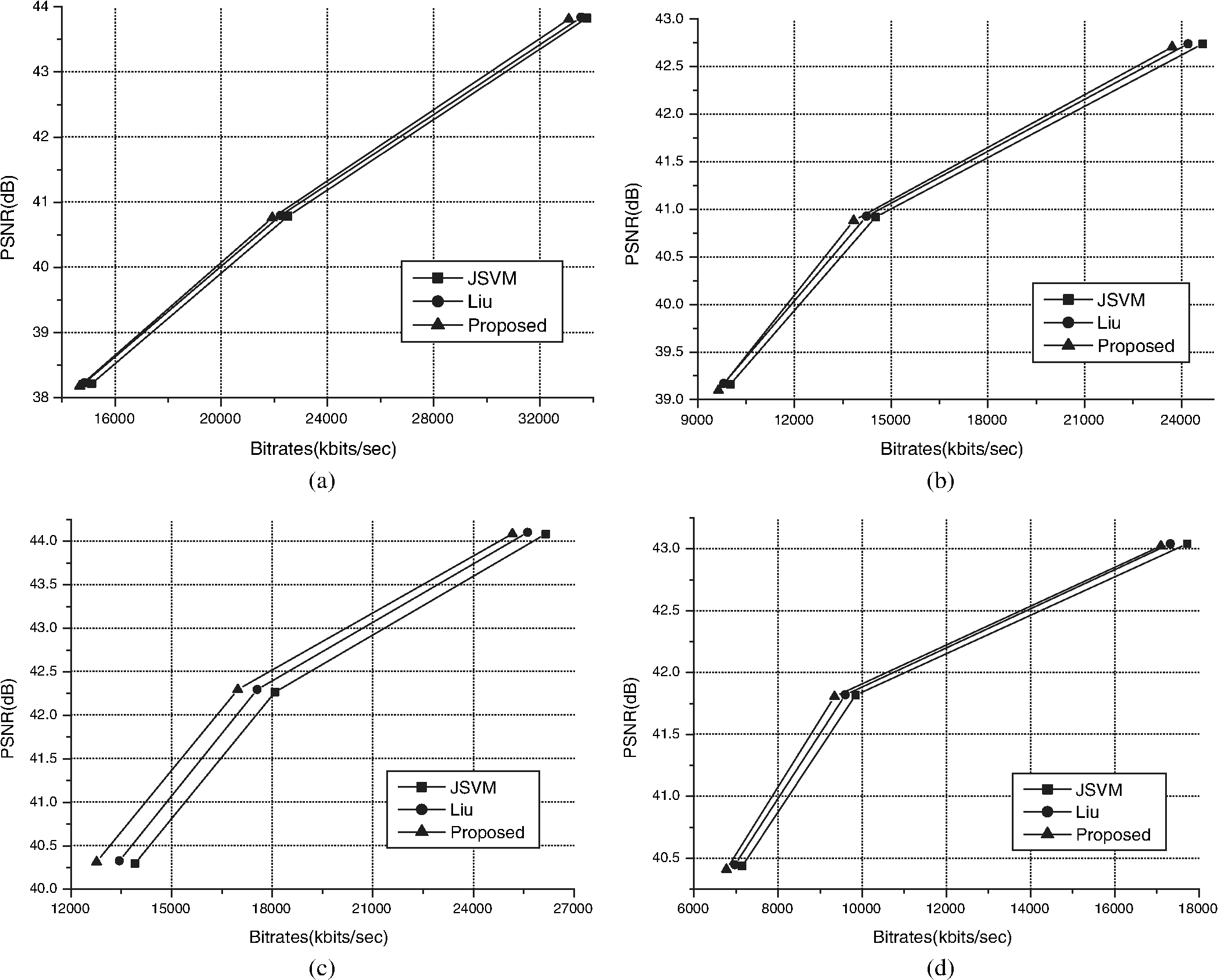

We also measured the encoding time of the proposed SILHIP method. Simulation results shows that the complexity of the proposed method varies depending on the sequences. In Table 2, the average encoding time of the CIF and 4CIF sequences is slightly increased by 13.78%. And, for the 1080p sequences, the average encoding time is increased by 14.72%. We can see that the encoding time increase of the proposed SILHIP method is slightly higher at the high resolution sequences.

6. Conclusion

A new SILHIP scheme to improve the coding efficiency of the EL coding of the SVC video was proposed. To adapt to the local features of an image block, the proposed SILHIP scheme calculates an edge map of the target block using the intensity gradient. Then a hybrid intra-prediction signal is constructed by using the edge map. Simulation results showed that the proposed SILHIP algorithm outperforms the state-of-the-art EL prediction in the SVC standard.

References

1.

T. Wiegandet al., “Joint draft 11 of SVC amendment,” (2007). Google Scholar

2.

H. SchwarzD. MarpeT. Wiegand, “Overview of the scalable video coding extension of the H.264/AVC standard,” IEEE Trans. Circuits Syst. Video Technol., 17 (9), 1103 –1120 (2007). http://dx.doi.org/10.1109/TCSVT.2007.905532 ITCTEM 1051-8215 Google Scholar

3.

T. H. Wanget al., “Computation-scalable algorithm for scalable video coding,” IEEE Trans. Consum. Electron., 57 (3), 1194 –1202 (2011). http://dx.doi.org/10.1109/TCE.2011.6018874 ITCEDA 0098-3063 Google Scholar

4.

C. Daiet al., “Geometry-adaptive block partitioning for intra-prediction in image & video coding,” in IEEE Int. Conf. on Image Process., 85 –88 (2007). Google Scholar

5.

T. Wiegandet al., “Overview of the H.264/AVC video coding standard,” IEEE Trans. Circuits Syst. Video Technol., 13 (7), 560 –576 (2003). http://dx.doi.org/10.1109/TCSVT.2003.815165 ITCTEM 1051-8215 Google Scholar

6.

C. S. ParkC. K. ParkS. J. Ko, “Generalization of interlayer intra-prediction for scalable video coding,” Electron. Lett., 44 (5), 337 –338 (2008). http://dx.doi.org/10.1049/el:20083114 ELLEAK 0013-5194 Google Scholar

7.

D. Liuet al., “Edge-oriented uniform intra-prediction,” IEEE Trans. Image Process., 17 (10), 1827 –1836 (2008). http://dx.doi.org/10.1109/TIP.2008.2002835 IIPRE4 1057-7149 Google Scholar

8.

K. BharanitharanB. D. LiuJ. F. Yang, “An efficient region based intra-prediction algorithm for H.264/Advanced video coding,” in Int. Conf. on Computer and Electrical Eng., 393 –397 (2008). Google Scholar

9.

Z. Wanget al., “Inter layer intra-prediction using lower layer information for spatial scalability,” Lecture Notes Control Inform. Sci., 345 303 –311 (2006). http://dx.doi.org/10.1007/978-3-540-37258-5 0170-8643 Google Scholar

10.

Y. LiuG. RathC. Guillemot, “Improved intra-prediction for H.264/AVC scalable extension,” in IEEE 9th Workshop on Multimedia Signal Processing. MMSP 2007 , 247 –250 (2007). Google Scholar

11.

C. S. Parket al., “Estimation-based interlayer intra-prediction for scalable video coding,” IEEE Trans. Circuits Syst. Video Technol., 19 (12), 1902 –1907 (2009). http://dx.doi.org/10.1109/TCSVT.2009.2026945 ITCTEM 1051-8215 Google Scholar

12.

J. S. StahlS. Wang, “Edge grouping combining boundary and region information,” IEEE Trans. Image Process., 16 (10), 2590 –2606 (2007). http://dx.doi.org/10.1109/TIP.2007.904463 IIPRE4 1057-7149 Google Scholar

13.

F. DestrempesM. Mignotte, “A statistical model for contours in images,” IEEE Trans. Pattern Anal. Mach. Intell., 26 (5), 626 –638 (2004). http://dx.doi.org/10.1109/TPAMI.2004.1273940 ITPIDJ 0162-8828 Google Scholar

14.

H. LiK. N. NganZ. Wei, “Fast and efficient method for block edge classification and its application in H.264/AVC video coding,” IEEE Trans. Circuits Syst. Video Technol., 18 (6), 756 –768 (2008). http://dx.doi.org/10.1109/TCSVT.2008.918778 ITCTEM 1051-8215 Google Scholar

15.

O. Divorraet al., “Geometry-adaptive block partitioning for video coding,” in Proc. ICASSP, 657 –660 (2007). Google Scholar

16.

Y. L. LeeK. H. HanG. J. Sullivan, “Improved lossless intra coding for H.264/MPEG-4 AVC,” IEEE Trans. Image Process., 15 (9), 2610 –2616 (2006). http://dx.doi.org/10.1109/TIP.2006.877396 IIPRE4 1057-7149 Google Scholar

17.

H. HuangT. Y. CaoX. W. Zhang, “The enhanced intra-prediction algorithm for H.264,” in Congress on Image and Signal Processing. CISP ’08, 161 –165 (2008). Google Scholar

18.

J. ReichelH. SchwarzM. Wien, (2007). Google Scholar

Biography and photograph of the author is not available.

CC BY: © The Authors. Published by SPIE under a Creative Commons Attribution 4.0 Unported License. Distribution or reproduction of this work in whole or in part requires full attribution of the original publication, including its DOI.

Citation Download Citation

Chun-Su Park "Spatial and interlayer hybrid intra-prediction for H.264/SVC video," Optical Engineering 52(7), 071503 (4 March 2013). https://doi.org/10.1117/1.OE.52.7.071503

Published: 4 March 2013

Access the abstract

JOURNAL ARTICLE
8 PAGES

DOWNLOAD PAPER SAVE TO MY LIBRARY

GET CITATION

CITATIONS

Cited by 2 scholarly publications and 1 patent.

Explore citations on Lens.org

KEYWORDS

Scalable video coding

Electroluminescence

Video

Image segmentation

Edge detection

Computer programming

Optical engineering

1.

Introduction

2.

Review of Previous Work and Basic Idea