Digital holographic measurements of shape and three-dimensional sound-induced displacements of tympanic membrane

Morteza Khaleghi; Weina Lu; Ivo Dobrev; Jeffrey Tao Cheng; Cosme Furlong; John Rosowski

doi:10.1117/1.OE.52.10.101916

17 July 2013 Digital holographic measurements of shape and three-dimensional sound-induced displacements of tympanic membrane

Morteza Khaleghi, Weina Lu, Ivo Dobrev, Jeffrey Tao Cheng, Cosme Furlong, John Rosowski

Author Affiliations +

Optical Engineering, Vol. 52, Issue 10, 101916 (July 2013). https://doi.org/10.1117/1.OE.52.10.101916

Abstract

Acoustically induced vibrations of the tympanic membrane (TM) play a primary role in the hearing process, in that these motions are the initial mechanical response of the ear to airborne sound. Characterization of the shape and three-dimensional (3-D) displacement patterns of the TM is a crucial step to a better understanding of the complicated mechanics of sound reception by the ear. Sound-induced 3-D displacements of the TM are estimated from shape and one-dimensional displacements measured in cadaveric chinchillas using a lensless dual-wavelength digital holography system (DWDHS). The DWDHS consists of laser delivery, optical head, and computing platform subsystems. Shape measurements are performed in double-exposure mode with the use of two wavelengths of a tunable laser, while nanometer-scale displacements are measured along a single sensitivity direction with a constant wavelength. Taking into consideration the geometrical and dimensional constrains imposed by the anatomy of the TM, we combine principles of thin-shell theory together with displacement measurements along a single sensitivity vector and TM surface shape to extract the three principal components of displacement in the full-field-of-view. We test, validate, and identify limitations of this approach via the application of finite element method to artificial geometries.

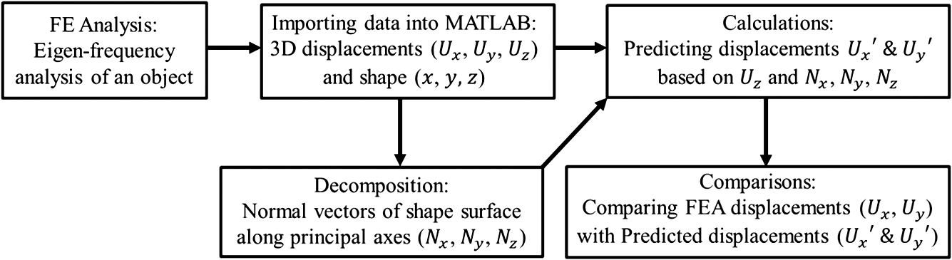
1. Introduction

The tympanic membrane (TM) is an essential part of the terrestrial vertebrate middle ear. Its function as an acousto-mechanical transformer greatly increases the sensitivity of the ear to sound.¹ Despite the importance of the TM, the relationship between its structure and its sound-reception function is not fully understood. Current methodologies for characterization of TM function in the laboratory and clinic have limitations: time-averaged holography is qualitative rather than quantitative, laser-Doppler vibrometry is usually limited to single-point (or a series of single-point) measurements of mobility, and most measurement techniques only measure displacements along a single direction. Furthermore, none of the current clinical tools for diagnosis of hearing losses measure the shape of the TM and the question of how shape affects function is an open question.²

The shape of the TM has been measured by different optical techniques (e.g., Moiré interferometry³^,⁴^,⁵ and fringe projection⁶). However, the temporal resolution and sensitivity of such three-dimensional (3-D) shape measurements are usually not sufficient to accurately measure the sound-induced motions of the TM. The lack of an accurate tool for simultaneous measurements of shape and 3-D vibrations of the TM is problematic. Conventional methods to measure the full-field 3-D displacements of the TM need at least three illumination or observation directions to realize three sensitivity vectors.⁷^,⁸ In this paper, a new technique is proposed to determine the full-field 3-D displacement components of the TM based on its shape and one-dimensional (1-D) displacement measurements.²^,⁹ The shape of the TM is measured by a lensless dual-wavelength digital holography system (DWDHS) that uses a tunable near-infrared laser. Concurrently, 1-D displacement measurements of acoustically induced motion of the TM are obtained by stroboscopic holography with a single laser wavelength and parallel illumination-observation recording geometry. Decomposing the shape’s normal vector at each point on the surface of the TM into three orthogonal axes, combining the shape information with the 1-D displacement at each point on the surface of the TM, and taking advantage of thin-shell theory principles allow estimation of the full 3-D displacement at each point on the surface of the TM. Therefore, a single, compact otoscope system could determine both the shape and 3-D acoustically induced displacement components of the TM.

2. Theoretical Considerations

2.1.

TM as a Thin-Shell

The shape, planar dimensions, and thickness of the TM vary among various vertebrate species.¹⁰ For human TM, Uebo et al.¹¹ measured mean thickness values between 50 and 150 μm in several TMs of humans of different ages. Ruah et al.¹² measured thicknesses at different regions of several TMs of humans aged between two days and 91 years. In adults the thickness varied between individuals and within regions: the pars flaccida varied from 80 to 600 μm, the posterosuperior pars tensa from 100 to 500 μm, posteroinferior tensa from 20 to 200 μm, anterosuperior tensa from 50 to 340 μm, anteroinferior tensa from 30 to 430 μm, and the umbo from 820 to 1700 μm. Decraemer and Funnell¹⁰ measured the thickness of the TM of three different species, including cats, gerbils, and humans, by confocal microscopy. For cats, the measured thickness was 12.5 to 60 μm; for gerbils, 7 to 70 μm; and for humans, 115 to 145 μm. Aernouts et al.¹³ measured the thickness of the human TM by confocal microscopy and found variations between 97 and 110 μm.

Can we think of the TM as a thin-shell? Novozhilov¹⁴ developed an engineering criterion that classifies a shell as thin if the following condition is satisfied:

Eq. (1)

\max (\frac{h}{R}) \leq 0.05,

where

h

is the thickness of the shell and

R

its radius of curvature. For chinchilla TM, a radius of curvature of 3.95 mm is obtained by the method proposed by Funnell.¹⁵ In all of the references cited in this paper this ratio is much smaller than 0.05, except around the manubrium, where the membrane is thicker; therefore, we modeled as a thin-shell.

According to plate and shell theory, and specifically considering Kirchhoff’s assumptions,¹⁶ in an elastic, homogenous, and isotropic thin-shell, where the displacement at any point of the shell is small compared with the thickness of the shell, (1) the displacement at any point on the surface of the membrane is perpendicular to the middle surface of the membrane and remains normal to it during and after deformation and (2) there is no displacement tangent to the surface of the membrane.

Although the TM is not strictly homogenous and isotropic, it is often approximated as such.¹⁰

2.2.

Lensless Digital Holography

Digital holography enables quantitative measurements of shape and displacements of objects by recording holograms with digital cameras and reconstructing them numerically. This allows imaging and focusing capabilities at arbitrary locations without the need of optical lenses and corresponding mechanisms. The Fresnel–Kirchhoff integral, Eq. (2), is used for holographic numerical reconstruction.¹⁷^,¹⁸

Eq. (2)

Γ (ξ, η) = \frac{i}{λ} \iint_{- \infty}^{+ \infty} h (x, y) R (x, y) \frac{\exp (- i \frac{2 π}{λ} ρ)}{ρ} \times (\frac{1}{2} + \frac{1}{2} \cos θ) d x d y,

Eq. (3)

ρ = \sqrt{{(x - ξ)}^{2} + {(y - η)}^{2} + d^{2}},

where

λ

is the wavelength of the laser,

h (x, y)

is the complex hologram function,

R (x, y)

is the complex amplitude distribution of the reference wave used for the reconstruction,

ρ

, which is expanded in Eq. (3), is the distance between a point on the hologram plane

(x, y)

and a point in the reconstruction plane

(ξ, η)

, and

d

is the reconstruction distance. The DWDHS discretizes and digitizes the function

Γ (ξ, η)

in Eq. (2) to the form of Eq. (4), by sampling the hologram function

h (x, y)

on a CCD sensor of

M \times N

pixels.

Eq. (4)

Γ (m, n) = \frac{i}{λ d} \exp [- i π λ d (\frac{m^{2}}{M^{2} Δ x^{2}} + \frac{n^{2}}{N^{2} Δ y^{2}})] \times \sum_{k = 0}^{M - 1} \sum_{l = 0}^{N - 1} h (k, l) R (k, l) \times \exp [- i \frac{π}{λ d} (k^{2} Δ x^{2} + l^{2} Δ y^{2})] \times \exp [i 2 π (\frac{k m}{M} + \frac{\ln}{N})],

where

m

and

n

are coordinates in the reconstruction plane,

k

and

l

are coordinates in the CCD plane,

M

and

N

are number of pixels of the CCD sensor, and

Δ x

and

Δ y

are the pixel dimensions. Figure 1 illustrates numerical reconstructions at specific distances from the CCD sensor of a digitally recorded hologram corresponding to a chinchilla TM stimulated with a tone of 7 kHz at 91 dB sound pressure level (SPL).

Fig. 1

Recording and numerical reconstruction of a digital hologram at specific distances from the CCD detector. Numerical reconstruction, performed at video rates, enables imaging and focusing capabilities without the need of optical elements. The object of interest is a chinchilla TM stimulated with a tone of 7 kHz at 91 dB SPL.¹⁹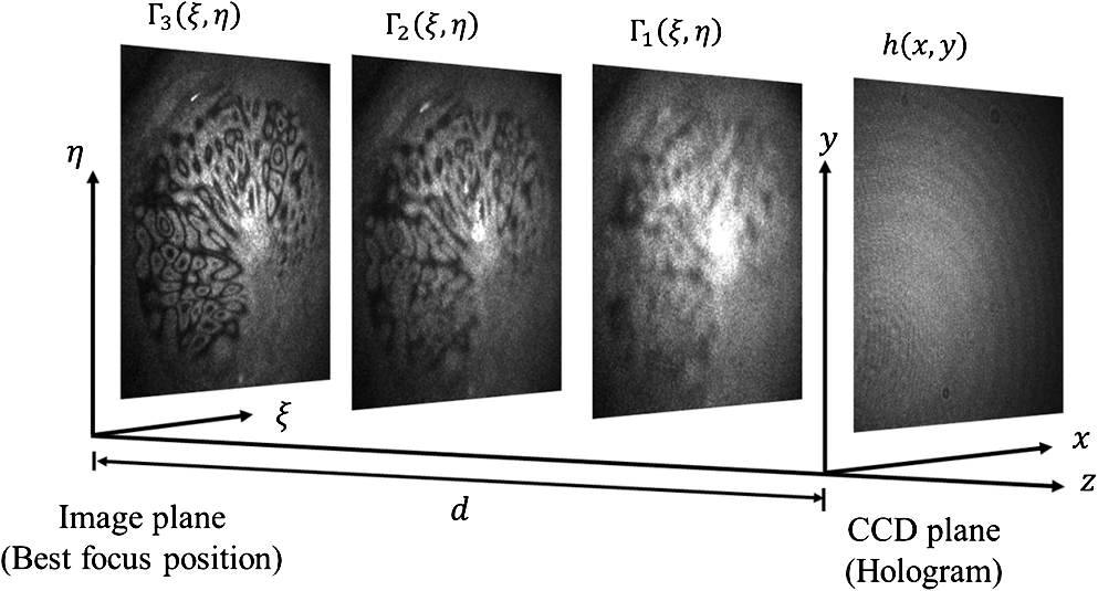

2.2.1.

Shape measurements by dual-wavelength digital holography

A two-wavelength holographic contouring technique is applied to generate depth contours related to the geometry of the TM. The technique is based on the utilization of a coherent polarized light source with wavelength tuning capabilities.²⁰ The technique requires acquisition of a set of optical amplitude and phase information at wavelength $λ_{1}$ , the reference state, as well as acquisition of a second set of amplitude and phase information at wavelength $λ_{2}$ , the deformed state. Interferometric depth contours, related to the geometry of the TM under investigation, are generated by speckle phase correlation of two sets of phase-stepped speckle intensity patterns.

The phase difference of the two corresponding sets of data $Δ ϕ$ is given by

Eq. (5)

Δ ϕ = ϕ_{2} - ϕ_{1} = \frac{2 π}{Λ} OPL,

where

ϕ_{1}

is the phase of the optical path length recorded at the first wavelength

λ_{1}

,

ϕ_{2}

is the phase of the optical path length recorded at the second wavelength

λ_{2}

, OPL is the optical path length defined as the distance from the illumination point to an object point and to an observation point, and

Λ

is the synthetic wavelength given by

Eq. (6)

Λ = \frac{λ_{1} λ_{2}}{| λ_{1} - λ_{2} |} .

From Eq. (6), it is clear that the smaller the difference between the two wavelengths used, the larger the synthetic wavelength and, consequently, the smaller the optical phase difference.

In two-wavelength contouring, the phase difference, $Δ ϕ$ , is a discontinuous wrapped function varying in the interval $[- π, π]$ ; thus phase unwrapping algorithms are applied to obtain a continuous phase distribution called the fringe-locus function, $Ω (x, y)$ , for calculation of the relative height of each point on the surface of the object $Z (x, y)$ with

Eq. (7)

Z (x, y) = \frac{Ω (x, y) * Λ}{4 π} .

If the angle between illumination and the observation directions, $θ$ , is zero, the distance between two consecutive contours is

Eq. (8)

Δ z = \frac{Λ}{1 + \cos (θ)} = \frac{Λ}{2} .

2.2.2.

Full-field three-dimensional displacement measurements

Conventional methods for measurement of 3-D displacements of objects by holographic interferometry use at least three illumination points or three observation points to define three sensitivity vectors. We describe a new method that utilizes measurements of the 1-D sound-induced displacements along the optical ( $z$ ) axis together with the 3-D decompositions of shape information into surface normal vectors to calculate the displacements in the other two orthogonal directions ( $x$ and $y$ ). Figure 2 illustrates the algorithm we applied to compute the 3-D displacement maps.

Fig. 2

Algorithm used to extract 3-D components of displacement by measurements of shape and one component of displacement.

A double-exposure stroboscopic mode is used for quantitative measurements of displacements between two loading states. In stroboscopic holography mode, the computed optical phase change, which is related to displacement, is based on the difference between measurements corresponding to two different stimulus phases, where the phases are defined by the pulsing of the “strobe switch” (an acousto-optic modulator capable of high-frequency switching) that is phase-locked to the acoustic stimulus. In our measurements, the sinusoidal motion of the TM driven by a tone was determined from holograms of the TM that were gathered during strobed laser pulse illumination at each of eight evenly spaced stimulus phases ( $\emptyset = 0, \frac{π}{4}, \frac{π}{2}, \dots, \frac{7 π}{4}$ ). Each laser pulse has a duration of 5 to 10% of the period of the tonal stimulus. The result gives a difference between the two states in the form of a wrapped phase map. By considering our parallel illumination-observation experimental setup, only out-of-plane displacements along the optical axis can be measured. DWDHS records four images containing holographic patterns that result from the phase-shifting of the reference beam in steps of multiples of $π / 2$ , at both reference and deformed states. The intensities at each pixel measured by the camera at each of the four reference phase steps are $I_{1}, \dots, I_{4}$ in the reference state and $I_{1}^{'}, \dots, I_{4}^{'}$ in the deformed state. The optical phase difference between these two states is

Eq. (9)

Ω (x, y) = \tan^{- 1} [- \frac{(I_{1} - I_{3}) (I_{4}^{'} - I_{2}^{'}) - (I_{4} - I_{2}) (I_{1}^{'} - I_{3}^{'})}{(I_{1} - I_{3}) (I_{1}^{'} - I_{3}^{'}) + (I_{4} - I_{2}) (I_{4}^{'} - I_{2}^{'})}],

which enables the measurements of out-of-plane displacement by

Eq. (10)

U_{z} (x, y) = \frac{Ω (x, y) * λ}{4 π} .

The hypothesis that the major components of acoustically induced displacements occur along the local surface normal of the TM makes it possible to recover the two principal components of TM motion in the plane of the tympanic ring, ${\vec{U}}_{x}$ and ${\vec{U}}_{y}$ in a Cartesian coordinate system defined by the corresponding sensitivity vector, as shown in Fig. 3. Specifically, single-axis measurements, ${\vec{U}}_{Z}$ , together with the knowledge of shape normal vectors, $\vec{n} ({\vec{n}}_{x}, {\vec{n}}_{y}, {\vec{n}}_{z})$ , enable estimation of the two additional corresponding orthogonal components of displacement, ${\vec{U}}_{x}$ and ${\vec{U}}_{y}$ , with

Eq. (11)

{\vec{U}}_{x} = {\vec{n}}_{x} \frac{| {\vec{U}}_{z} |}{| {\vec{n}}_{z} |},

Eq. (12)

{\vec{U}}_{y} = {\vec{n}}_{y} \frac{| {\vec{U}}_{z} |}{| {\vec{n}}_{z} |} .

Fig. 3

Decomposition of the surface normal vector and resultant displacement at one point: (a) $\vec{n}$ is the surface normal vector and ${\vec{n}}_{x}$ , ${\vec{n}}_{y}$ , and ${\vec{n}}_{z}$ are decomposed components of $\vec{n}$ along $x$ , $y$ and $z$ axes. (b) $\vec{U}$ is the resultant displacement and ${\vec{U}}_{x}$ , ${\vec{U}}_{y}$ , and ${\vec{U}}_{z}$ are decomposed components of $\vec{U}$ along $x$ , $y$ and $z$ axes. $α$ , $β$ , and $γ$ are the angles between the direction of $\vec{U}$ or $\vec{n}$ an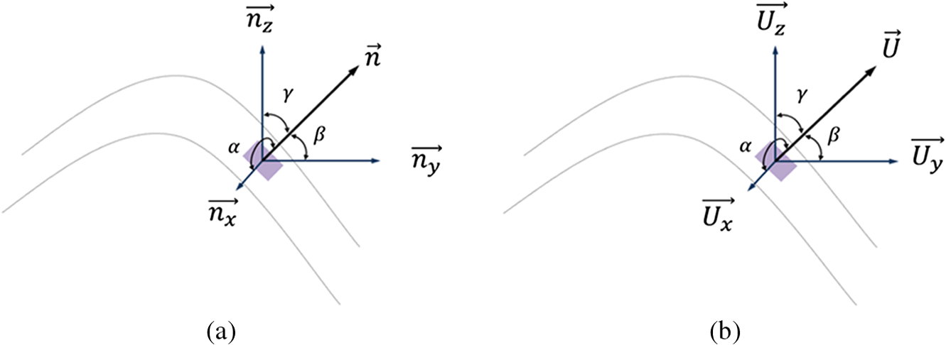d the $x$ , $y$ , $z$ axes.

As illustrated in Fig. 3, angles between displacement in $x$ , $y$ , $z$ directions and the resultant displacement are the same as angles between the normal vectors in $x$ , $y$ , $z$ directions and the normal vector.

2.3.

Test of the Proposed Approach

In order to test our approach, a finite element method (FEM) modal analysis of an ideal semi-spherical membrane with physical properties similar to those of a TM is implemented and the results imported and processed in MATLAB. Figure 4 shows the test procedures, while the geometry, mechanical properties, and modeling parameters incorporated into the finite element analysis (FEA) model analyses are listed in Table 1.

Fig. 4

Procedure for testing our approach by FEM simulations.

Table 1

Geometry, mechanical properties, and FEM parameters of the semi-spherical test object.

Geometry		Mechanical properties		FEA parameters
Spherical radius	2.5 mm	Young’s modulus	60 MPa	No. of nodes	15,697
Thickness	30 μm	Poisson’s ratio	0.33	No. of elements	7747
Thickness	30 μm	Mass density	$1100 kg / m^{3}$	No. of elements	7747

Note: Boundary conditions: fully constrained along entire perimeter.

Outputs of the FEM modal analysis are the resultant displacement, ${\vec{U}}_{res}$ , as well as displacement along the $x$ , $y$ and $z$ axes. By taking the fourth mode of vibration, for example, and by applying Eqs. (11) and (12), the two additional displacements ${\vec{U}}_{x}$ and ${\vec{U}}_{y}$ are calculated and plotted in Fig. 5.

Fig. 5

Computed $x$ and $y$ components of displacements obtained by applying our approach: (a) Predicted displacement along $x$ -axis ( ${\vec{U}}_{x}$ ). (b) Predicted displacement along 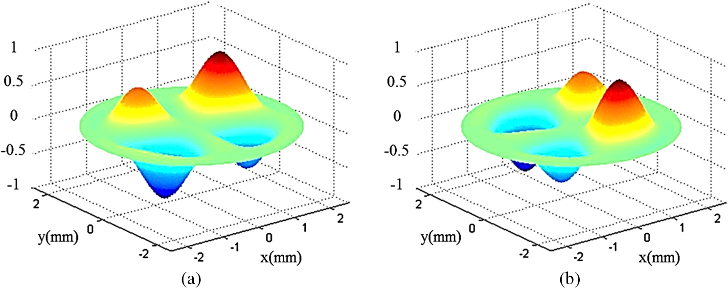$y$ -axis ( ${\vec{U}}_{y}$ ).

A significant criterion used in the testing of our approach is the computation of the differences between the displacements obtained from the FEM analysis and the predicted components based on the thin-shell hypothesis. These differences are shown in Fig. 6. Because of the nature of the eigenvectors obtained by FEM, data from each FEM solution and prediction are normalized by the maximal displacement value on the TM surface.

Fig. 6

Comparisons of $x$ and $y$ components of displacements between FEM solutions ( ${\vec{U}}_{x}$ and ${\vec{U}}_{y}$ ) and predictions obtained by our approach after data normalization.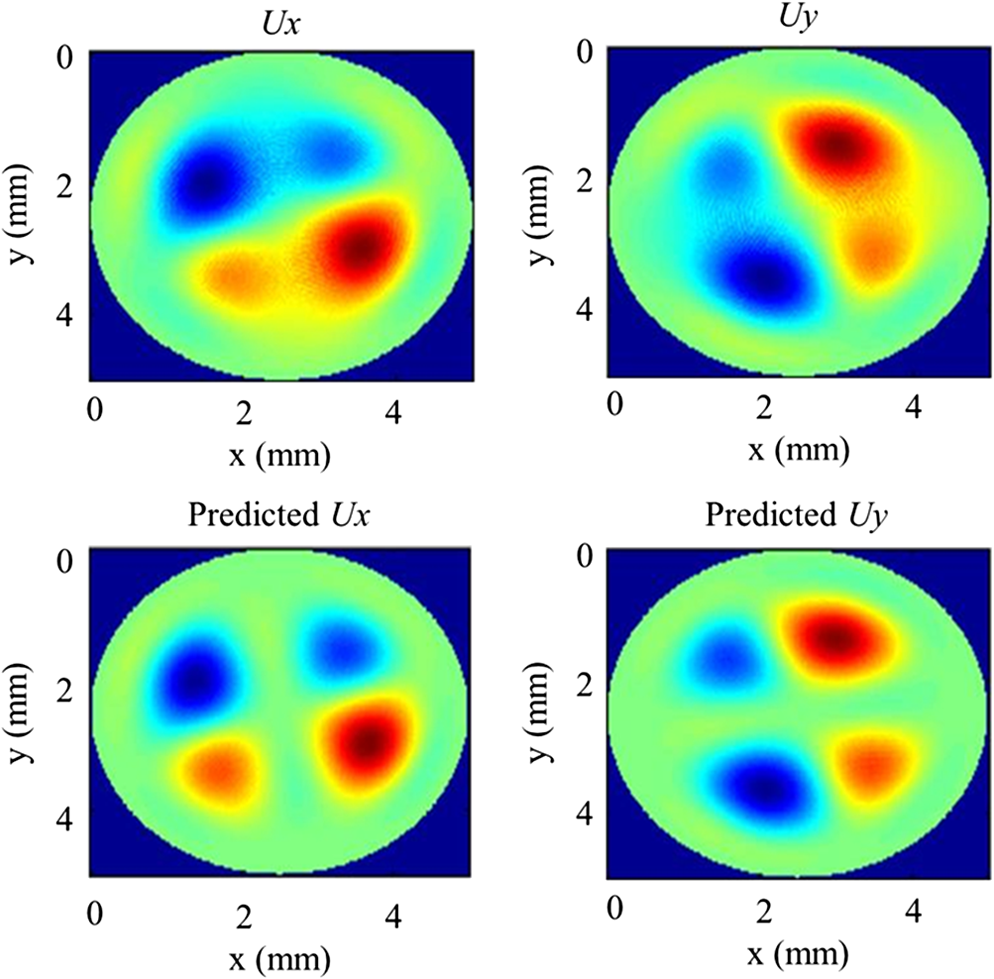

Table 2 shows the root mean square (RMS) and standard deviation of the differences between FEM and predicted displacements averaged over the surface for different modes of vibration after data normalization. The results show that the RMS difference and the standard deviation around the mean is less than 5%, which indicates that the predicted $x$ and $y$ displacement components obtained by our approach are well matched by the displacements obtained by FEM analysis.

Table 2

Root mean square (RMS) and standard deviation (SD) of the difference between FEM solutions and predictions for different modes of vibration for the ideal semi-spherical test object.

Difference		Mode 1	Mode 2	Mode 3	Mode 4
$x$	RMS (%)	3.08	3.52	3.18	0.71
$x$	STD (%)	3.10	4.18	2.91	0.90
$y$	RMS (%)	3.11	3.38	3.52	0.71
	STD (%)	3.12	3.07	4.30	0.91

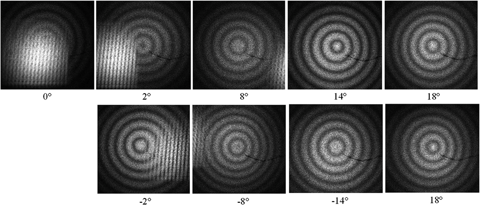
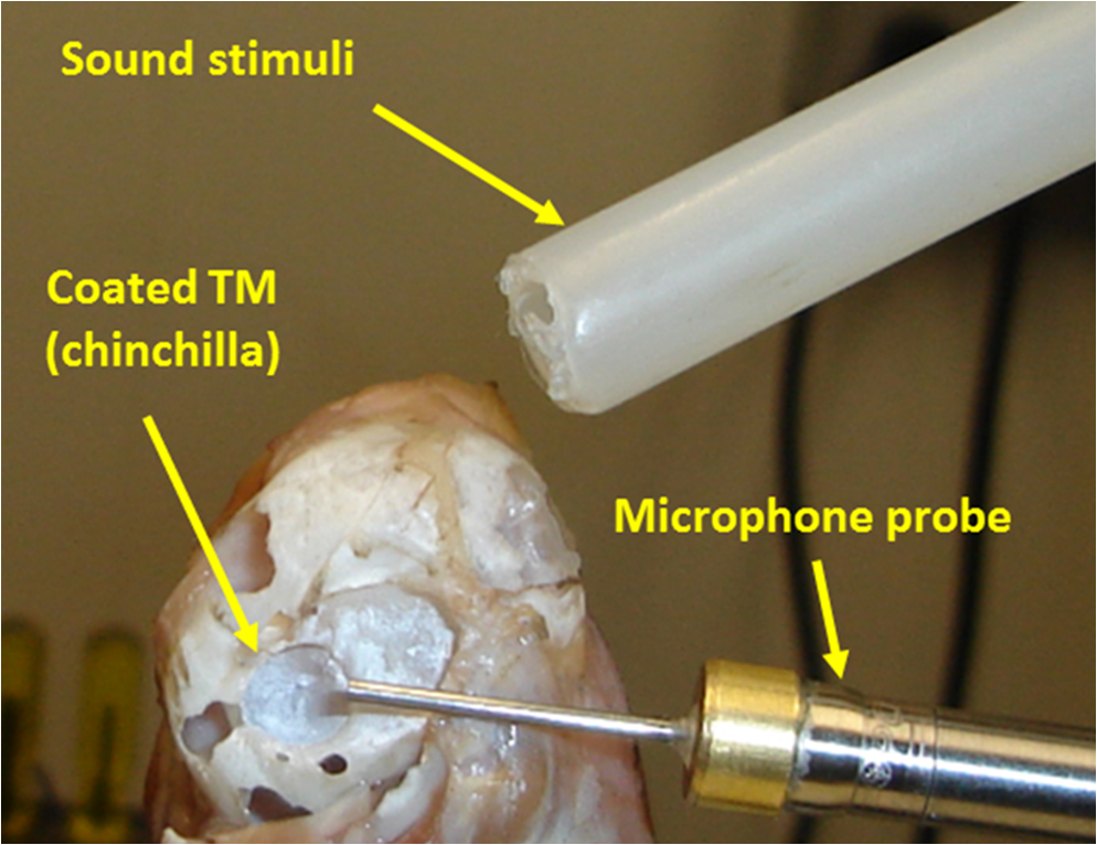
3. Experimental Procedures

3.1.

Digital Optoelectronic Holography System

The lensless DWDHS consists of laser delivery (LD), optical head (OH), and computing platform (CP) subsystems. The LD subsystem contains a tunable near-infrared diode laser in the range from 770 to 789 nm with a central wavelength of 779 nm, an anamorphic prism pair, an acousto-optic modulator, a half-wave plate, and a fiber coupler assembly. The output of LD is delivered to the OH directly. The OH was designed using 3-D optical ray tracing simulations, in which selected components are rotated in specific angles to overcome reflection issues.²¹ A 5 megapixel ( $2452 \times 2054 pixels$ ) digital camera with pixel size of 3.45 by $3.45 {μ m}^{2}$ in OH is used for image recording at high rates, while the CP acquires and processes images in either time-averaged or double-exposure modes.²² Figure 7 shows the major components of the DWDHS.

Fig. 7

Schematic views of different subsystems of our DWDHS. Laser delivery consists of an infrared tunable laser, acousto-optic modulator, mirror, and laser to fiber coupler; optical head contains a modified Michelson interferometer; and computing platform controls the recording parameter such as sound-excitation level and frequency, phase-shifting, synchronizations for stroboscopic measurements and all the acquisition parameters. The dashed lines are analog signal lines and digital control and sense lines.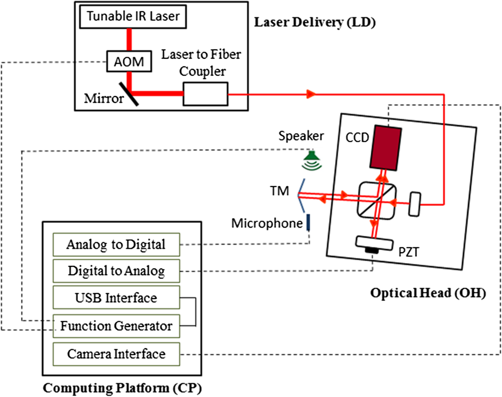

3.2.

Design of Optical Head Subsystem

The OH subsystem is based on a Michelson optical configuration, shown in Fig. 8. The input to the interferometer is a single-mode polarization-maintaining fiber terminated with an fiber-optic connector/angled physical contact connector that attaches to a collimator ( $C$ ) producing a circular beam of 7.1 mm diameter. The collimated beam is directed to a nonpolarizing broadband (700 to 1100 nm) beam splitter cube (BC) that splits the light into reference and object beams. A neutral density filter (NDF) and a linear polarizer ( $P$ ) are embedded on the optical path of the reference beam to control the beam ratio; the ratio has an optimal value between 2 and 5 and depends on the reflectivity of the tested sample. NDF provides coarse adjustment and the P fine adjustment. There are no components in the optical path of the object beam since we utilize lensless digital holographic methods. The reflected reference and object wavefronts are combined at the CCD sensor and a piezoelectric transducer is used for temporal phase-shifting.

Fig. 8

Computer aided design (CAD) models of the designed and implemented optical head: (a) Assembled package showing characteristic dimensions. (b) View showing its principal components. PZT, piezoelectric transducer; $M$ , mirror; $p$ , linear polarizer; NDF, neutral density filter; BC, beam splitter cube; CCD, digital camera; $C$ , collimating lens with fiber-optic (FC) connector for optical fiber input; and $O$ , object.

In our initial OH configurations, we observed that the BC can introduce significant internal reflections that affect the quality of the reconstructed digital holograms. Therefore, the geometry of the interferometer was modified by applying rotations to some of the components within the optical path of the reference beam in order to identify a suitable optical configuration. In Fig. 8, the original axis describing the location of all parts is shown by the vertical dotted line. The BC was rotated by an angle of $α$ with respect to the vertical axis, and the mirror, $M$ , and CCD camera were rotated by $2 α$ in order to maintain the mirror and the camera parallel to each other. The angle $α$ was changed from $- 18$ to $+ 18 \deg$ in 2-deg increments. The resultant numerically reconstructed²³^,²⁴ digital holograms obtained after applying these rotations are shown in Fig. 9. Selected images with interference fringes generated on a conical metal object for shape measurements are shown. Marks on the object were introduced to help numerical focusing of the object. While significant reflections degraded the holograms measured at $α$ between $+ 18$ and $- 18 \deg$ , good quality, low-reflection holograms were obtained at larger angles. By quantifying image intensity and contrast, it was determined that 14 deg was a suitable choice.

Fig. 9

Comparison of interferogram quality corresponding to different optomechanical configurations used during optimization of the OH by changing the incident angle of the BC. The configuration corresponding to 14 deg rotation was chosen in the final configuration.

3.3.

Sound Generation and Measurement

In displacement measurement experiments, the TM is excited by a sound source. The sinusoidal output of the function generator was amplified by a unity gain power amplifier and used to drive a dynamic speaker coupled to an inverted horn. The narrow mouth of the horn was positioned about 8 cm away from the TM. A PCB Piezotronics (Depew, New York) prepolarized 1/4-inch microphone with a calibrated probe tube was positioned just at the edge of the TM to measure the SPL. In the experiments, sinusoidal sound stimuli varied in frequency from 414 to 10,000 Hz with levels between 70 and 120 dB SPL.

3.4.

Sample Preparation

The heads of chinchillas used in other physiological experiments were harvested from dead animals. The bilateral bullae were exposed and the bullar walls partially removed to expose the tympanic cavity. The cartilaginous ear canals were resected, and the bony external auditory canals were drilled away until 80 to 90% of the TM surface was visible.⁹^,²⁵ When using laser imaging, it is essential that the surface upon which the beams are emitted is reflective enough to produce a good clean image. Due to the translucent nature of the TM, the surface of the membrane needs to be coated with a suitable material to increase the light reflection from the surface. While there are many chemical compounds that could be used to paint the TM, most are unsuitable due to concerns and limitations regarding what is permissible for future use in the human TM.²⁶

First, the coating must not be toxic or cause any inflammation or irritation to the skin. Second, there must be a safe method for applying and removing the coating. Beyond health concerns, there are also concerns about what impact the coating will have on the results of the experiments. If the coating is too thick or too rigid, it may affect how the membrane vibrates, leading to incorrect measurements.²⁷ Third, the coating needs to be highly reflective, specifically within the wavelength region of the laser that is used during the experiments (780 nm). Last, the coating needs to be evenly distributed on the membrane, as any large-scale unevenness could alter the vibration patterns or the quality of the reflected light.²⁶ Based on literature²⁸ and the experience from physicians and researchers at the Massachusetts Eye and Ear Infirmary, zinc oxide (ZnO) was used as paint. ZnO is commonly used in cosmetics, is highly reflective, and is soluble in weak acetic acid for easy removal from the membrane. Figure 10 shows a coated TM of a chinchilla subjected to the sound stimuli in a displacement measurement test.

Fig. 10

Chinchilla’s TM is coated with zinc oxide to increase light reflection. The TM is shown surrounded by the bone of the middle-ear wall. The placement of the tube conducting sound to the ear and the probe microphone are also illustrated.

4. Results

4.1.

Shape and Surface Normal Vectors

The shape of a chinchilla’s TM measured by DWDHS is shown in Figs. 11 and 12. Figure 11 shows the masked and filtered wrapped optical phase of the shape of the TM obtained by dual-wavelength double exposure. In these measurements, the first exposure (reference state) was captured at the wavelength of 779.8 nm and the second exposure (deformed state) at 780.2 nm, leading to a synthetic wavelength of 1.52 mm, a little smaller than the depth of the TM cone.

Fig. 11

Masked and filtered wrapped optical phase of the shape of the TM, computed by lensless DWDHS.⁹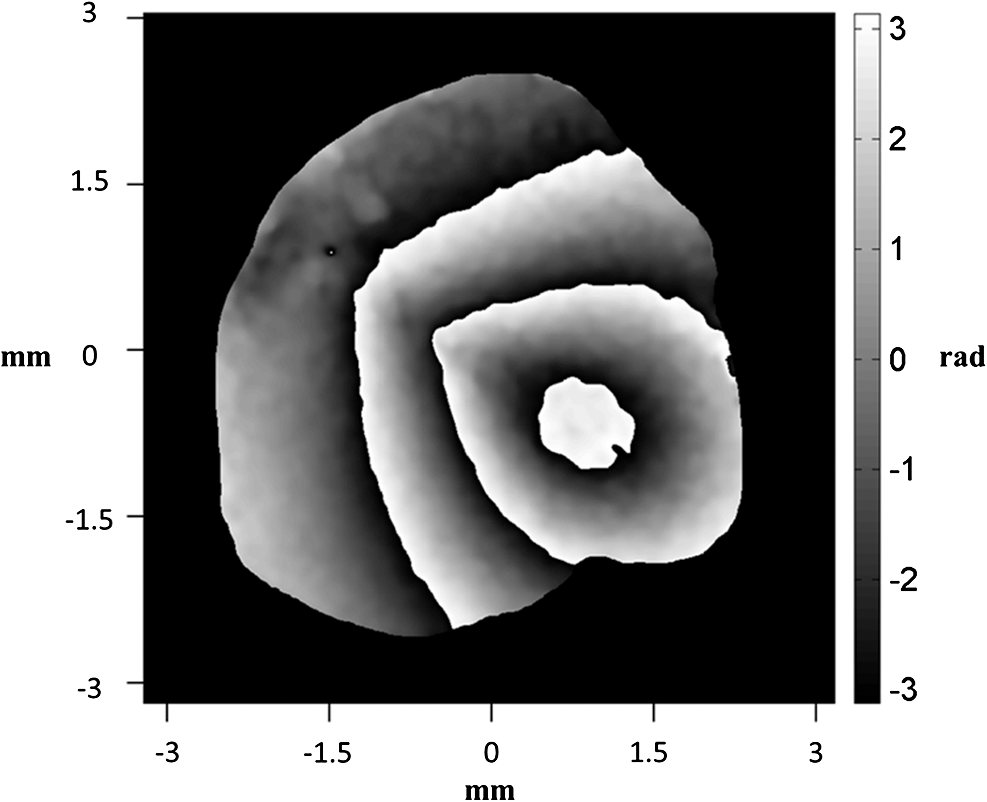

Fig. 12

Measured shape of the TM of a chinchilla: (a) Three-dimensional shape. (b) Two-dimensional side view of the shape. (c) Two-dimensional top view of the shape; the outline of the entire tympanic ring is highlighted by a circle. The outline shows the handle of the malleus (the manubrium). The umbo of the manubrium is at the apex of the TM cone.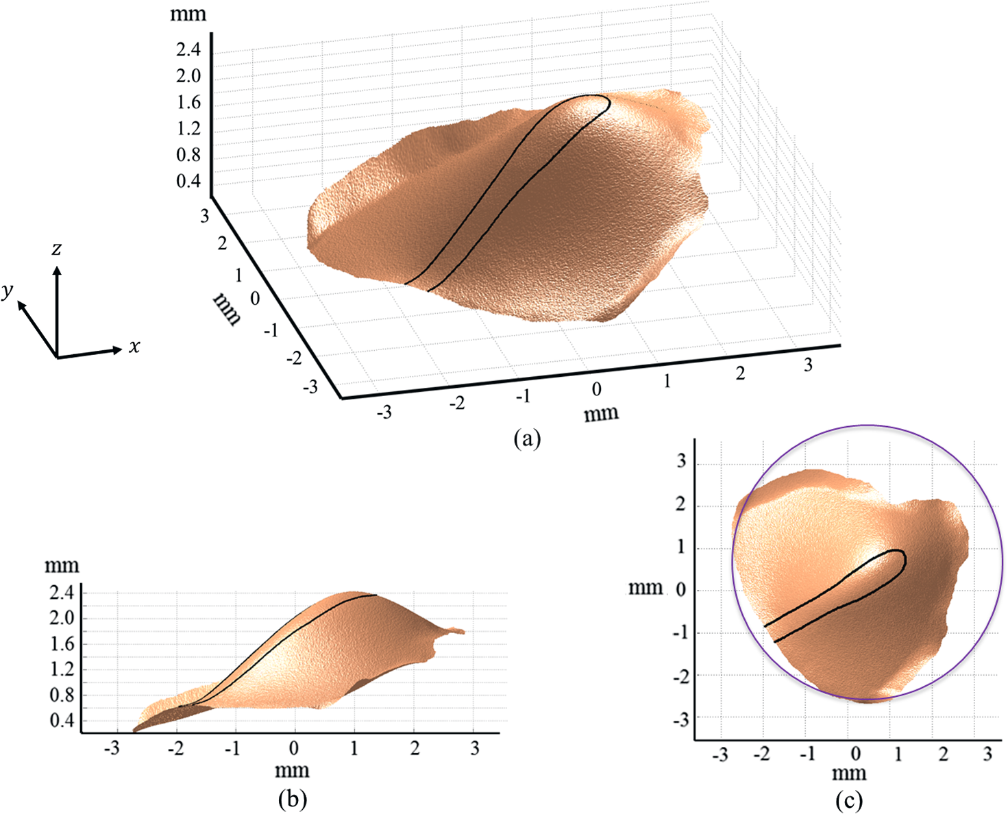

Figure 12 shows the unwrapped scaled image of the optical phase that quantifies the shape of the lateral surface of the TM, where a $z$ value of 0 corresponds to the location of the bony rim that supports the TM and larger $z$ values code a deeper location within the ear. The outline of the handle of the malleus (the manubrium) embedded in the medial surface of the TM is also illustrated. The depth of the membrane (from the umbo to the rim) is about 2.4 mm and the diameter of the membrane is about 7 mm. Because it is not possible to completely remove the bony canal that surrounds the TM, the image does not reconstruct the entire surface; this limitation is most severe at values of $x \in (1 ∶ 3)$ and $y \in (1 ∶ 3)$ , which correspond to more ventral (inferior) portions of the TM.

The principal components of the surface normal vector along the three orthogonal $x$ , $y$ , and $z$ observation axes are obtained by vector decomposition of the surface normal vector as shown in Fig. 3(a). The results of this decomposition are shown in Fig. 13. Since the umbo is located at the apex of the TM cone, the surface at the umbo is nearly parallel to the TM ring and orthogonal to the observation direction that defines the $z$ axis. Therefore, the normal vector at the umbo is dominated by its $z$ -component ( $z$ -component near 1, and significantly small $x$ and $y$ components). Also note that the cone-like shape of the TM and the near match between the $z$ -projection and the axis of the cone yields $z$ -components that are all positive, while the $x$ - and $y$ - components may be negative or positive depending on the spatial gradient of the membrane surface in $x$ and $y$ .⁹

Fig. 13

Principal components of surface normals along $x$ -axis (a), $y$ -axis (b), and $z$ -axis (c).⁹ The outline shows the handle of the malleus (the manubrium).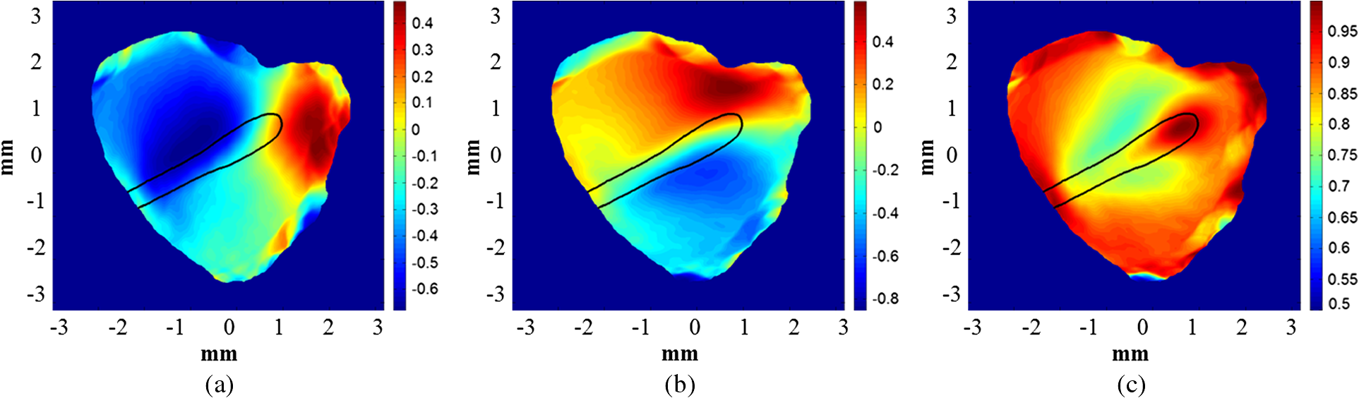

4.2.

One-Dimensional Displacement Measurements Along One Optical Axis

Sinusoidal continuous sound stimuli were applied to the membrane and the displacements of the surface were recorded and computed at six frequencies of interest: 414, 1000, 2500, 5730, 8735, and 10,000 Hz with SPLs between 100 and 122 dB. The levels were selected to produce measurable sound-induced TM displacements.

Stroboscopic holography was used to measure TM motions. In stroboscopic holography, the acousto-optic modulator contained within the DWDHS strobes the laser, so that the object and the CCD are illuminated by a series of brief pulses. Each pulse is 5 to 10% of the period of each cycle of the acoustic stimulus, and within each camera frame the pulses are locked to a single phase of the stimulus cycle. Each camera image then represents the summed response to a large number of strobe impulses that are all locked to the same stimulus phase. To describe the variations in TM displacement with the phase of the stimulus, a holographic image (each calculated from four images with stepped optical phase of the reference beam) was gathered at each of the eight stimulus phases of either $0, 45, 90 \dots 315 \deg$ relative to the zero-crossing of the sinusoidal voltage that drives the earphone.²⁹^,³⁰

Figure 14 shows out-of-plane ( $z$ -axis) displacements of the TM at different stimulus frequencies. The vibration patterns are categorized based on the sound excitation frequency. The vibrational pattern of 414 Hz is simple, which is characterized by one or two spatial maxima. The vibrational patterns of 1000 and 2500 Hz are complex,²⁵ which are characterized by multiple spatial maxima and minima separated by areas of small displacement. Above 4 kHz, the displacement patterns of chinchilla TM are ordered, which are characterized by many small areas of maximal displacement around the manubrium, with some order to the location of the maxima.

Fig. 14

Out-of-plane or $z$ -axis peak displacements measured at six different frequencies by DWDHS. Displacements are in the unit of μm.⁹

4.3.

Recovering the Three Components of Displacement

By applying Eqs. (11) and (12), and the measured $z$ -axis component of displacement ( $U_{z}$ ), and taking advantage of the corresponding normal vectors extracted from the measured shape, the $x$ -axis ( $U_{x}$ ), $y$ -axis ( $U_{y}$ ), and resultant ( $U_{res}$ ) components of displacement are calculated. To help identify the computed 3-D components of displacement on the TM surface, these displacements are overlaid on the measured 3-D shape of the TM for one of the experiments in which a sound stimulus of 5730 Hz and 101 dB SPL sound level stimulates the TM, as shown in Fig. 15, which demonstrates that the $x$ and $y$ components of displacement ( $U_{x}$ and $U_{y}$ ) are smaller than the out-of-plane component ( $U_{z}$ ). The resultant displacement has a maximum value within the posterior-inferior quadrant of the TM.

Fig. 15

Principal components of displacement along three orthogonal axes of the TM as obtained by application of our approach. TM was subjected to sound stimuli of 5730 Hz and sound pressure level of 101 dB: (a) 3-D view. (b) 2-D top view. The $z$ axis corresponds to the lateral-medial direction with medial as positive, which was defined by the longitudinal axis of the illuminating and reflected laser beam. The $x$ direction is approximate to the rostral (anterior)-caudal (posterior) axis with rostral positive. The $y$ direction is approximate to the dorsal (superior)-ventral (inferior) direction with ventral positive. Displacements are in the unit of μm.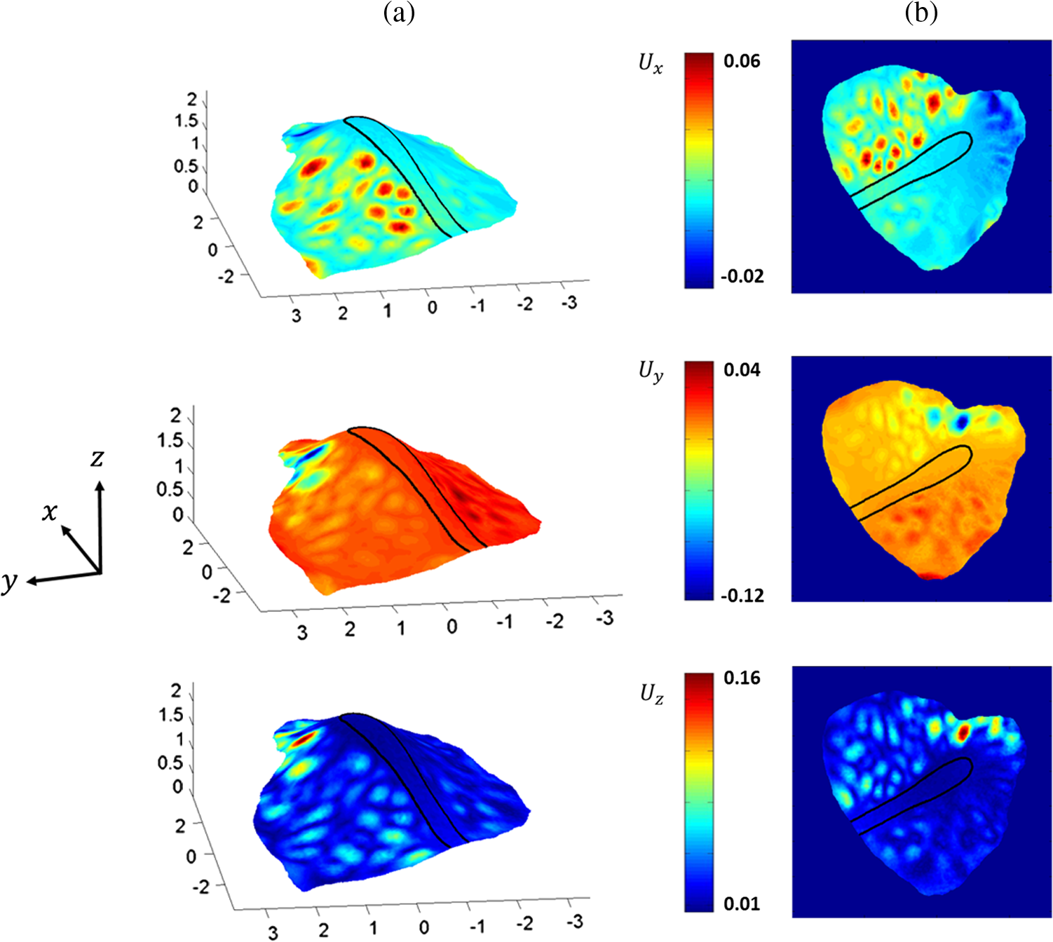

5. Conclusions

We presented a new approach to measure 3-D displacements of TM by combining shape information and 1-D components of displacement. Shape and displacement measurements are carried out with a lensless DWDHS, with shape measured in two-wavelengths mode and 1-D displacements measured in single-wavelength mode. The assumptions we used in our computation of the 3-D components of displacement from measured shape and 1-D displacements are based on considering the TM as a thin-shell, so that the principal components of TM vibration are hypothesized to be parallel to the principal components of the normal vectors of the surface of the TM. This approach was tested using FEM models. However, further testing of our approach will be performed in the next steps of this research, including the development of improved FEM models as well as direct measurements of $x$ , $y$ components of displacement by other digital holographic methods that involve speckle correlation and multiple sensitivity vectors. We expect that our efforts toward the development of methodologies for the concurrent measurement of shape and the three components of displacement vectors will lead to realizable full-field-of-view tools for the study of the normal and pathologic middle-ears.

Acknowledgments

This work was supported by the National Institute on Deafness and Other Communication Disorders, the Mass Eye & Ear Infirmary, and the Worcester Polytechnic Institute, Mechanical Engineering Department. We would also like to acknowledge the support of all of the members of the Center for Holographic Studies and Laser micro-mechaTronics laboratories and particularly of Peter Hefti and Ellery Harrington.

References

1.

J. TonndorfS. M. Khanna, “The tympanic membrane as a part of the middle ear transformer,” Acta Oto-laryngologica, 71 (1–6), 177 –180 (1971). http://dx.doi.org/10.3109/00016487109125347 AOLAAJ 0001-6489 Google Scholar

2.

W. Lu, “Development of a multi-wavelength lensless digital holography system for 3D deformations and shape measurements of tympanic membranes,” Mechanical Engineering Department, Worcester Polytechnic Institute, (2012). Google Scholar

3.

W. F. DecraemerJ. J. J. DirckxW. R. J. Funnell, “Shape and derived geometrical parameters of the adult, human tympanic membrane measured with a phase-shift Moiré interferometer,” Hear. Res., 51 (1), 107 –122 (1991). http://dx.doi.org/10.1016/0378-5955(91)90010-7 HERED3 0378-5955 Google Scholar

4.

J. J. J. DirckxW. F. Decraemer, “Phase shift Moiré apparatus for automatic 3-D surface measurement,” Rev. Sci. Inst., 60 (12), 3698 –3701 (1989). http://dx.doi.org/10.1063/1.1140477 RSINAK 0034-6748 Google Scholar

5.

J. J. J. DirckxW. F. Decraemer, “Moiré topography for basic and clinical hearing research,” Rec. Devel. Opt., 3 271 –296 (2003). Google Scholar

6.

J. Liang, “Determination of the mechanical properties of guinea pig tympanic membrane using combined fringe projection and simulation,” Mechanical Engineering Department, Oklahoma State University, (2009). Google Scholar

7.

R. J. PryputniewiczW. W. Bowley, “Techniques of holographic displacement measurement: an experimental comparison,” App. Opt., 17 (11), 1748 –1756 (1978). http://dx.doi.org/10.1364/AO.17.001748 APOPAI 0003-6935 Google Scholar

8.

M. Khaleghiet al., “3-Dimensional quantification of surface shape and acoustically-induced vibrations of TM by digital holography,” in Proc. FRINGE 2013, (2013). Google Scholar

9.

J. J. Rosowskiet al., “Measurements of three-dimensional shape and sound-induced motion of the chinchilla tympanic membrane,” Hear. Res., 301 44 –52 (2013). http://dx.doi.org/10.1016/j.heares.2012.11.022 HERED3 0378-5955 Google Scholar

10.

W. F. DecraemerW. R. J. Funnell, “Anatomical and mechanical properties of the tympanic membrane,” Chronic Otitis Media. Pathogenesis-Oriented Therapeutic Management, 51 –84 Kugler Publications, The Netherlands (2008). Google Scholar

11.

K. Ueboet al., “Thickness of normal human tympanic membrane,” Ear. Res. Jpn., 19 70 –73 (1988). Google Scholar

12.

C. B. Ruahet al., “Age-related morphologic changes in the human tympanic membrane,” Arch. Otolaryngol. Head and Neck Surg., 117 (6), 627 –634 (1991). http://dx.doi.org/10.1001/archotol.1991.01870180063013 AONSEJ 0886-4470 Google Scholar

13.

J. AernoutsJ. R. M. AertsJ. J. J. Dirckx, “Mechanical properties of human tympanic membrane in the quasi-static regime from in situ point indentation measurements,” Hear. Res., 290 (1–2), 45 –54 (2012). http://dx.doi.org/10.1016/j.heares.2012.05.001 HERED3 0378-5955 Google Scholar

14.

V. V. Novozhilov, Theory of Thin Elastic Shells, 2nd ed.P. Noordhoff, Groningen, The Netherlands (1964). Google Scholar

15.

W. R. J. Funnell, “A theoretical study of eardrum vibrations using the finite-element method,” Department of Electrical Engineering, McGill University, (1975). Google Scholar

16.

A. E. H. Love, “On the small free vibrations and deformations of elastic shells,” Philos. Trans. R. Soc. A, 179 491 –549 (1888). http://dx.doi.org/10.1098/rsta.1888.0016 PTRMAD 1364-503X Google Scholar

17.

U. SchnarsW. Jüptner, “Digital recording and numerical reconstruction of holograms,” Meas. Sci. Technol., 13 (9), 85 –101 (2002). http://dx.doi.org/10.1088/0957-0233/13/9/201 MSTCEP 0957-0233 Google Scholar

18.

E. KolenovicC. FurlongW. Jüptner, “Inspection of micro-optical components by novel digital holographic techniques,” Proc. SEM, 470 –475 (2004). Google Scholar

19.

I. Dobrevet al., “Digital holographic otoscope for measurements of the human tympanic membrane in-vivo,” Proc. SPIE, 8494 849409 (2012). http://dx.doi.org/10.1117/12.954633 PSISDG 0277-786X Google Scholar

20.

C. FurlongR. J. Pryputniewicz, “Absolute shape measurements using high-resolution optoelectronic holography methods,” Opt. Eng., 39 (1), 216 –223 (2000). http://dx.doi.org/10.1117/1.602355 OPEGAR 0091-3286 Google Scholar

21.

TracePro, Littleton, MA (2012). Google Scholar

22.

E. Harringtonet al., “Automatic acquisition and processing of large sets of holographic measurements in medical research,” Proc. SEM, 5 219 –228 (2011). http://dx.doi.org/10.1007/978-1-4614-0228-2 2191-5644 Google Scholar

23.

J. M. Flores-Morenoet al., “Holographic otoscope for nano-displacement measurements of surfaces under dynamic excitation,” Scanning, 33 (5), 342 –352 (2011). http://dx.doi.org/10.1002/sca.v33.5 SCNNDF 0161-0457 Google Scholar

24.

C. Furlonget al., “Assessing eardrum deformation by digital holography,” J. Biomed. Opt. Med. Imag., (2013). http://dx.doi.org/10.1117/2.1201212.004612 Google Scholar

25.

J. J. Rosowskiet al., “Computer-assisted time-averaged holography of the motion of the surface of the tympanic membrane with sound stimuli of 0.4 to 25 kHz,” Hear. Res., 253 (1–2), 83 –96 (2009). http://dx.doi.org/10.1016/j.heares.2009.03.010 HERED3 0378-5955 Google Scholar

26.

S. Goldishet al., “Packaging and optimization of a digital holographic otoscope for clinical use,” Mechanical Engineering Department, Worcester Polytechnic Institute, (2010). Google Scholar

27.

J. T. Chenget al., “Wave motion on the surface of the human tympanic membrane: holographic measurement and modeling analysis,” JASA, 133 (2), 918 –937 (2013). http://dx.doi.org/10.1121/1.4773263 JASMAN 0001-4966 Google Scholar

28.

J. J. J. DirckxW. F. Decraemer, “Optoelectronic Moiré projector for real-time shape and deformation studies of the tympanic membrane,” J. Biomed. Opt., 2 (2), 176 –185 (1997). http://dx.doi.org/10.1117/12.268966 JBOPFO 1083-3668 Google Scholar

29.

J. T. Chenget al., “Motion of the surface of the human tympanic membrane measured with stroboscopic holography,” Hear. Res., 263 (1–2), 66 –77 (2010). http://dx.doi.org/10.1016/j.heares.2009.12.024 HERED3 0378-5955 Google Scholar

30.

C. Furlonget al., “Miniaturization as a key factor to the development and application of advanced metrology systems,” Proc. SPIE, 8413 84130T (2012). http://dx.doi.org/10.1117/12.981668 PSISDG 0277-786X Google Scholar

Biography

Morteza Khaleghi received his MSc degree in mechanical and manufacturing engineering from Iran University of Science and Technology. Currently, he is pursuing his PhD degree at Worcester Polytechnic Institute (WPI), Worcester, Massachusetts. He is a research assistant at the Center for Holographic Studies and Laser micro-mechaTronics (CHSLT) of WPI. His research interests include developments of 3-D optical metrology systems, medical imaging, and digital image processing.

Weina Lu received her BS degree in environmental engineering from University of Science and Technology Beijing, Beijing, China, in 2009, and her MSc degree in mechanical engineering from WPI, Massachusetts, in 2012. Since then, she has been working at the Wellman Center for Photomedicine at Massachusetts General Hospital in the field of biomedical optics.

Ivo Dobrev received his BS degrees in mechanical engineering and robotics engineering from WPI in Worcester, Massachusetts, in 2009. He is currently a PhD candidate in the mechanical engineering department of WPI. He is a graduate research assistant at the CHSLT of WPI. His research interests include high-speed optical metrology in field environment and in vivo, lensless digital holography, shearography, structured light measurements, transient measurements, digital image processing, haptic control and mechatronics, system design and integration.

Jeffrey Tao Cheng is an instructor in otology and laryngology at Harvard Medical School, working on middle-ear mechanics and tissue biomechanics through measurements and modeling.

Cosme Furlong is an associate professor of mechanical engineering, working in mechanics, optical metrology, and nanoengineering, science and technology.

John J. Rosowski is a professor of otology and laryngology, and also of health sciences and technology, working in acoustics and mechanics of the external, middle, and inner ear, as well as the comparative middle and external ear structure and function.

CC BY: © The Authors. Published by SPIE under a Creative Commons Attribution 4.0 Unported License. Distribution or reproduction of this work in whole or in part requires full attribution of the original publication, including its DOI.

Citation Download Citation

Morteza Khaleghi, Weina Lu, Ivo Dobrev, Jeffrey Tao Cheng, Cosme Furlong, and John Rosowski "Digital holographic measurements of shape and three-dimensional sound-induced displacements of tympanic membrane," Optical Engineering 52(10), 101916 (17 July 2013). https://doi.org/10.1117/1.OE.52.10.101916

Published: 17 July 2013

Access the abstract

JOURNAL ARTICLE
12 PAGES

DOWNLOAD PAPER SAVE TO MY LIBRARY

GET CITATION

CITATIONS

Cited by 37 scholarly publications.

Explore citations on Lens.org

KEYWORDS

Digital holography

Holography

Finite element methods

Ear

Holograms

Optical engineering

3D metrology

1.

Introduction

2.

Theoretical Considerations

2.1.

TM as a Thin-Shell

Eq. (1)

2.2.

Lensless Digital Holography

Eq. (2)

Eq. (3)

Eq. (4)

Fig. 1

2.2.1.

Shape measurements by dual-wavelength digital holography

Eq. (5)

Eq. (6)

Eq. (7)

Eq. (8)

2.2.2.

Full-field three-dimensional displacement measurements

Fig. 2

Eq. (9)

Eq. (10)

Eq. (11)

Eq. (12)

Fig. 3

2.3.

Test of the Proposed Approach

Fig. 4

Table 1

Fig. 5

Fig. 6

Table 2

3.

Experimental Procedures

3.1.

Digital Optoelectronic Holography System

Fig. 7

3.2.

Design of Optical Head Subsystem

Fig. 8

Fig. 9

3.3.

Sound Generation and Measurement

3.4.

Sample Preparation

Fig. 10

4.

Results

4.1.

Shape and Surface Normal Vectors

Fig. 11

Fig. 12

Fig. 13

4.2.

One-Dimensional Displacement Measurements Along One Optical Axis

Fig. 14

4.3.

Recovering the Three Components of Displacement

Fig. 15

5.

Conclusions

Acknowledgments

References

Biography

Show All Keywords

Keywords/Phrases

Search In:

Publication Years