Optical moving target indicator for synthetic aperture radar images

Yuan Li; Gaohuan Lv

doi:10.1117/1.OE.52.8.083103

2 August 2013 Optical moving target indicator for synthetic aperture radar images

Yuan Li, Gaohuan Lv

Author Affiliations +

Optical Engineering, Vol. 52, Issue 8, 083103 (August 2013). https://doi.org/10.1117/1.OE.52.8.083103

Abstract

An optical indicator is designed to detect the moving targets in complex-valued synthetic aperture radar (SAR) images and estimate their azimuth velocity components. The indicator consists of two subsystems, and each of them is composed of one phase-only filter and two cylindrical lenses. The subsystems refocus the SAR image by changing the parameters of the phase-only filters to get two refocused images in which the background is defocused to the same extent while the moving targets are defocused differently. The indicator involved detects moving targets by comparing the sharpness of two defocused SAR images piece-by-piece, and then estimates the azimuth velocity of each detected target from its sharpness difference curve. The effectiveness of the optical architecture is investigated, and the proposal is confirmed by theoretical analysis and experiments with simulated and field data.

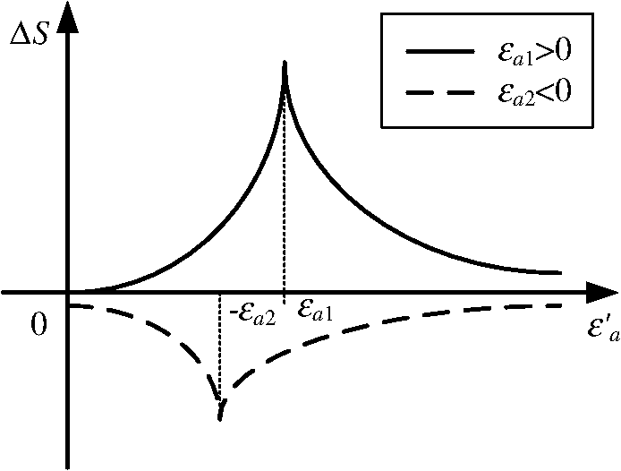
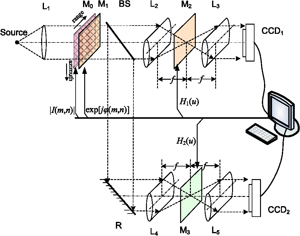
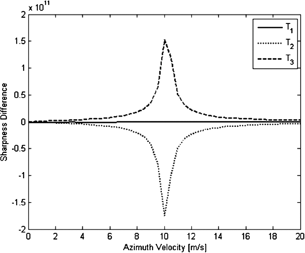
1. Introduction

Ground moving target indication plays an important role in the synthetic aperture radar (SAR) image processing community. For a moving point scatterer, the image is displaced in an azimuth dimension and then defocused in the range dimension due to its range velocity component. In addition, it is smeared in the azimuth dimension due to its azimuth velocity component. In the range Doppler domain of the returns from a moving target, the range velocity component leads to a nonzero Doppler centroid and the azimuth velocity component leads to a biased Doppler modulation rate with respect to that of the background. Researchers have exploited the affected phase information to identify the moving targets in a complex-valued SAR image.¹^–⁵

For a moving target with a nonzero range velocity component, it is possible for it to be detected by computing the Doppler centroid in the returns via pulse-by-pulse, and the corresponding algorithms, which are relatively mature.⁶^–⁸ For a target moving in the azimuth direction only, many methods have been proposed, such as shear-average based autofocusing,²^,³ information extraction from the antenna beam pattern,⁴ and image stack technology.⁵ Most of them are based on using phase estimation or Doppler filter-bank techniques. However, the traditional digital algorithms mainly concentrate on operations such as Fourier transformation and phase estimation. These algorithms are so complex that they are usually computationally expensive to implement. Furthermore, they are not robust enough to deal with clutters or interference.

As an optical cylindrical lens acts as a natural Fourier transform operator, it is used in many early SAR processors.⁹ In this paper, we will present an optical moving target indicator (MTI) to detect moving targets with nonzero azimuth velocities in a complex-valued SAR image, and show how to estimate their azimuth velocities.

Using our approach, two refocused SAR images are generated using two refocusing filters. In one refocused SAR image, a moving target will be in better focus, while in the other, it will be defocused. By comparing the sharpness of the two refocused SAR images, it is possible to identify the moving target.

Our optical MTI architecture uses two groups of refocusing subsystems. Each of the subsystems consists of two cylindrical lenses and one phase-only matching filter. The majority of this paper is a brief analytical description of the detection and azimuth velocity estimation methods that we used. The proposed architecture has been verified by both computer simulations and field data experiments. The results show that the optical processor is effective and practicable.

The paper is organized as follows. The principles for moving target detection and azimuth velocity estimation in the spatial domain of a given SAR image are reviewed. We then propose and discuss an optical processor using the detection and estimation principles. Both simulated and field data are used to verify the proposed scheme. Finally, we state our conclusion of the proposed concept.

2. Principles

2.1.

Moving Target Detection in Space Domain

A strip-map mode SAR is considered in the following analysis. For a stationary point scatterer, its azimuth phase history has the form:¹⁰

Eq. (1)

ϕ_{s} (x) = - π K_{a} x^{2},

where

x

is the azimuth coordinate, and

K_{a} = 2 / (λ R_{0})

with

λ

being the carrier wavelength and

R_{0}

being the slant range to the stationary scatterer. If a scatterer is moving in azimuth direction with a constant velocity

V_{a}

, then the azimuth signal becomes

Eq. (2)

s_{a} (x) = \exp [- j π K_{a} {(1 - ε_{a})}^{2} x^{2}], | x - x_{0} | \leq l_{s},

where

x_{0}

is the azimuth position of the moving scatterer when the radar bore-sight is directed to the scatterer,

l_{s}

is the synthetic aperture length, and

ε_{a} = V_{a} / V_{p}

with

V_{p}

being the platform velocity.

Taking the Fourier transform of $s_{a} (x)$ according to the stationary phase theory and ignoring the amplitude constant and the phase constant, one obtains

Eq. (3)

S_{a} (u) = \exp [j \frac{u^{2}}{4 π {(1 - ε_{a})}^{2} K_{a}}] \exp (- j u x_{0}), | u | \leq \frac{2 π}{l_{a}},

where

l_{a}

is the antenna length. Usually

| ε | ≪ 1

, so the following approximation can be made:

Eq. (4)

\frac{1}{{(1 - ε_{a})}^{2}} \approx 1 + 2 ε_{a} .

In the traditional range Doppler algorithm,¹¹ if $S_{a} (u)$ is filtered by

Eq. (5)

H (u) = \exp (- j \frac{u^{2}}{4 π K_{a}}),

then the focused version of

S_{a} (u)

is

Eq. (6)

S_{f} (u) = \exp (j \frac{ε_{a} u^{2}}{2 π K_{a}}) \exp (- j u x_{0}), | u | \leq \frac{2 π}{l_{a}} .

Taking the inverse Fourier transform of the above in Eq. (6), the focused signal can be shown to be

Eq. (7)

s_{f} (x) = s_{0} (x) ⋆ s_{r} (x),

where

Eq. (8)

s_{0} (x) = \frac{\sin [π \frac{2}{l_{a}} (x - x_{0})]}{π (x - x_{0})},

Eq. (9)

s_{r} (x) = F_{u \to x}^{- 1} [\exp (j \frac{ε_{a} u^{2}}{2 π K_{a}})], | u | \leq \frac{2 π}{l_{a}},

and the symbol

⋆

means the convolution operation. In Eq. (9),

F^{- 1}

denotes the inverse Fourier transform. According to the stationary phase theory, and neglecting the constant coefficient,

s_{r} (x)

takes the form

Eq. (10)

s_{r} (x) = \exp (j π \frac{K_{a} x^{2}}{2 ε_{a}}) .

Equation (10) indicates that a residual quadratic phase term appears in the refocused signal. This residual term affects the focusing effectiveness.

The effect of the residual quadratic phase is shown in Fig. 1. In Fig. 1(a), the solid line represents the time frequency distribution of a stationary target, the dotted line and the dashed line represent that of two moving targets with the negative and positive azimuth velocity component, respectively.

Fig. 1

Results of azimuth compression in Doppler domain. (a) Time–frequency representation of a stationary target and two moving targets. (b) Residual quadratic Doppler phase term after azimuth compression.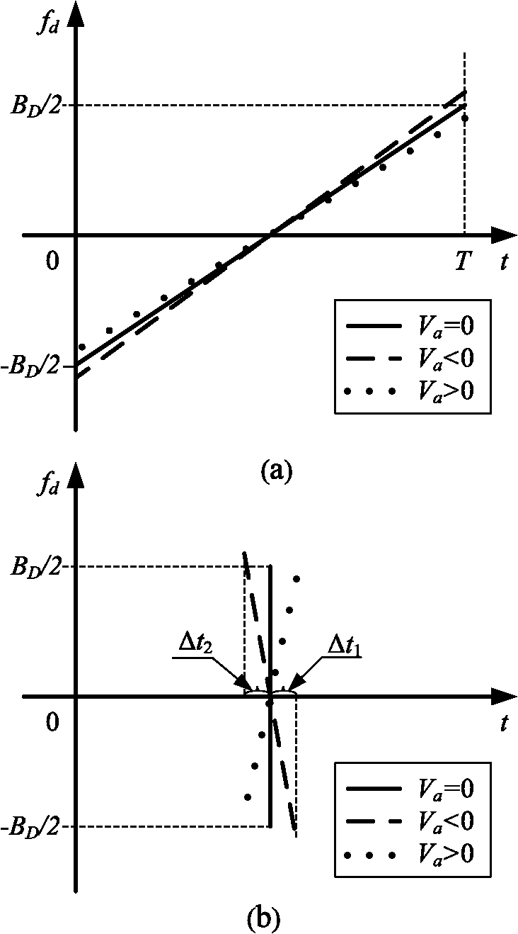

It can be seen that the Doppler chirp rate of a moving target varies with its azimuth velocity component. In the traditional range Doppler imaging algorithm, the azimuth matched filter is optimally designed for the stationary background, so when it is used to compress the azimuth signal history of a moving target, a residual quadratic Doppler phase appears as shown in Fig. 1(b). In this figure, after being compressed in azimuth, it can be seen that the quadratic Doppler phase term of a stationary target is ideally removed after azimuth compression, which means that the stationary target can be focused optimally.

For the two moving targets, as the residual quadratic Doppler phase terms exist, the compressed signal of the target with $ε_{a} > 0$ and that of the target with $ε_{a} < 0$ have the pulse width of $Δ t_{1}$ and $Δ t_{2}$ , respectively.

As the bandwidth of $s_{r} (x)$ is $4 π / l_{a}$ , its azimuth width in space domain satisfies

Eq. (11)

2 π \frac{K_{a}}{2 | ε_{a} |} Δ x = \frac{4 π}{l_{a}},

and thus

Eq. (12)

Δ x = | ε_{a} | μ_{x} \cdot ρ_{a},

where

μ_{x} = λ R_{0} / ρ_{a}^{2}

with

ρ_{a} = l_{a} / 2

being the theoretical azimuth resolution which is the effective space width of

s_{0} (x)

. The image of a moving scatterer will be smeared to the azimuth length

Eq. (13)

ρ_{smear} \approx (1 + | ε_{a} | μ_{x}) ρ_{a} .

If the SAR image is refocused in azimuth with a pair of new refocusing filters described by

Eq. (14)

H_{1} (u) = \exp (- j \frac{ε_{a}^{'} u^{2}}{2 π K_{a}}),

and

Eq. (15)

H_{2} (u) = \exp (j \frac{ε_{a}^{'} u^{2}}{2 π K_{a}}),

where

ε_{a}^{'} = V_{a}^{'} / V_{p}

with

V_{a}^{'}

is a probing azimuth velocity, then two refocused SAR images will be obtained. In the two refocused SAR images, the background is smeared to the same extent, while for a moving target, the two refocused Doppler spectra will be

Eq. (16)

S_{f 1} (u) = \exp [j \frac{u^{2}}{2 π K_{a}} (ε_{a} - ε_{a}^{'})] \exp (- j u x_{0}),

and

Eq. (17)

S_{f 2} (u) = \exp [j \frac{u^{2}}{2 π K_{a}} (ε_{a} + ε_{a}^{'})] \exp (- j u x_{0}) .

Equations (16) and (17) illustrate that the moving target will be smeared differently in the two refocused images. In one image it is focused better, while in another image it is defocused worse. For a quadratic phase error, in the smeared image the energy tends to be spread uniformly over the distance of the smear for an un-weighted aperture.² The moving target image will be in better focus when the refocused residual phase term is smaller, with the opposite also being true.

Different measurements can be used to describe the focusing quality, such as sharpness, entropy, and contrast. We adopt the sharpness function¹² defined by

Eq. (18)

D = \sum_{(m, n) \in P} {| g (m, n) |}^{4},

where

P

is a patch sized by a resolution cell. The moving target can be indicated by comparing the sharpness between the two refocused SAR images:

Eq. (19)

D_{c} = | D_{1} - D_{2} |,

where

D_{1}

and

D_{2}

are the sharpness distribution image of the two SAR images refocused by

H_{1} (u)

and

H_{2} (u)

, respectively. During the sharpness computation procedure, the patches are overlapping so that a moving target with a typical size will correspond to a set of bright pixels in the sharpness difference image. The bright pixels will be kept when a median filter is used to remove isolated bright pixels caused by noise.

2.2.

Azimuth Velocity Component Measurement

In Eq. (16), the refocused image is smeared in

Eq. (20)

M (ε_{a}, ε_{a}^{'}) = 1 + | ε_{a} - ε_{a}^{'} | μ_{x}

azimuth resolution cells, and in Eq. (17), the refocused image is smeared in

Eq. (21)

M (ε_{a}, - ε_{a}^{'}) = 1 + | ε_{a} + ε_{a}^{'} | μ_{x}

azimuth resolution cells. For a moving scatterer having the intensity

{| b |}^{2}

, its sharpness difference of the two refocused SAR images can be formulated by

Eq. (22)

D_{c} (ε_{a}, ε_{a}^{'}) = \frac{{| b |}^{4}}{M (ε_{a}, ε_{a}^{'})} - \frac{{| b |}^{4}}{M (ε_{a}, - ε_{a}^{'})} .

Equation (22) will be analyzed on the condition that $ε_{a}^{'} > 0$ . When $ε_{a} > 0$ , in the case of $0 < ε_{a}^{'} \leq ε_{a}$ ,

Eq. (23)

\frac{d D_{a}}{d ε_{a}^{'}} = \frac{{| b |}^{4} μ_{x}}{{[1 + μ_{x} (ε_{a} - ε_{a}^{'})]}^{2}} + \frac{{| b |}^{4} μ_{x}}{{[1 + μ_{x} (ε_{a} + ε_{a}^{'})]}^{2}} > 0 .

And in the case of $ε_{a}^{'} > ε_{a}$ ,

Eq. (24)

\frac{d D_{a}}{d ε_{a}^{'}} = \frac{{| b |}^{4} μ_{x}}{{[1 + μ_{x} (ε_{a} + ε_{a}^{'})]}^{2}} - \frac{{| b |}^{4} μ_{x}}{{[1 + μ_{x} (ε_{a}^{'} - ε_{a})]}^{2}} < 0 .

The two cases show that (1) when $0 < ε_{a}^{'} \leq ε_{a}$ , $D_{c} (ε_{a}, ε_{a}^{'})$ is a monotonic increasing function that reaches its maximum value at the point where $ε_{a}^{'} = ε_{a}$ , and (2) when $ε_{a}^{'} > ε_{a}$ , $D_{c} (ε_{a}, ε_{a}^{'})$ is a monotonic decreasing function that reaches its maximum value at the point where $ε_{a}^{'} = ε_{a}$ . In addition, it infinitely approaches zero with incremental increases of $ε_{a}^{'}$ .

The same analysis procedure can be repeated for the case of $ε_{a} < 0$ . The analysis results show that (1) when $0 < ε_{a}^{'} \leq - ε_{a}$ , $D_{c} (ε_{a}, ε_{a}^{'})$ is a monotonic decreasing function that reaches its minimum value at the point where $ε_{a}^{'} = - ε_{a}$ , and (2) when $ε_{a}^{'} > - ε_{a}$ , $D_{c} (ε_{a}, ε_{a}^{'})$ is a monotonic increasing function that reaches its minimum value at the point where $ε_{a}^{'} = - ε_{a}$ . In addition, the sharpness difference curve infinitely approaches zero with the increment of $ε_{a}^{'}$ .

Figure 2 presents two sharpness difference curves versus $ε_{a}^{'}$ for two moving targets with $ε_{a} > 0$ and $ε_{a} < 0$ , respectively. From this diagram, we can see that the azimuth velocity of a moving target can be estimated from its sharpness difference curve at the peak or valley point. The peak indicates that the target’s azimuth velocity component is positive, while the valley indicates a negative value.

Fig. 2

Sharpness difference curves of two moving targets in opposite azimuth direction.

The discussion above provides us a chance to estimate the azimuth velocity of a detected moving target by varying $ε_{a}^{'}$ in a reasonable range.

3. Implementation

The optical MTI processor architecture is presented in Fig. 3. In this architecture, a given complex-valued SAR image named $I (m, n)$ is separated into an amplitude part and a phase part in the computer, i.e.,

Eq. (25)

I (m, n) = | I (m, n) | \exp [j φ (m, n)],

where

φ (m, n)

is the phase angle of

I (m, n)

. Two spatial light modulators (SLM),

M_{0}

and

M_{1}

, are modulated by

| I (m, n) |

and

\exp [j φ (m, n)]

, respectively. The modulated light is split up into two beams by a beam-splitter. One beam is transmitted to the cylindrical lens

L_{2}

, the other part is reflected to the cylindrical lens

L_{4}

. The lenses

L_{2}

and

L_{4}

transform the complex-valued SAR image into a range Doppler map. The phase-only SLM

M_{2}

is modulated by the refocusing filter

H_{1} (u)

, and the filtered range Doppler map is transformed by the cylindrical lens

L_{3}

resulting in a refocused SAR image. The computer samples the refocused image by using a charge-coupled diode (CCD) camera. The same operations are performed at

L_{4}

,

M_{3}

, and

L_{5}

except that

M_{3}

is modulated by the refocusing filter

H_{2} (u)

. After the two refocused SAR images are sampled and stored, their sharpness difference is computed and the moving targets are indicated.

Fig. 3

An optical architecture to detect moving targets in a complex-valued SAR image.

Let us discuss the selection of $ε_{a}^{'}$ . For a moving target, either a too small or a too large $ε_{a}^{'}$ will lead to a small $D_{c}$ . To detect moving targets with different azimuth velocities, $ε_{a}^{'}$ will vary. For example, it can be orderly selected from a set $V_{a}^{'} = {5, 10, 15, 20, 25, 30} (m / s)$ .

After a moving target is detected, it is isolated from the given SAR image and sent to the SLMs $M_{0}$ and $M_{1}$ . By varying $ε_{a}^{'}$ , a series of refocusing filter pairs are generated and displayed in $M_{2}$ and $M_{3}$ . As a result, a sharpness difference curve is drawn in the computer. The target’s azimuth velocity can be estimated from this curve.

This scheme is feasible because the sharpness of clutter is erased from the sharpness difference image, and thus the moving target can be detected with greater ease. Furthermore, the optical architecture ensures high computational efficiency because complex Fourier transforms are implemented by lenses instead of digital computation.

4. Results

4.1.

Computer Simulation

We can verify the proposed scheme by computer simulations combined with optical instruments. In one of the simulations, three point scatterers are used as the scene. The three scatterers are set up such that one is stationary, and the other two have azimuth velocity components of $- 10$ and $10 m / s$ . The radar waveform is a chirp pulse, its bandwidth is 400 MHz, the pulse width is 20 μs, and the pulse repetition frequency is 2000 MHz. The radar carrier frequency is 10 GHz. While the radar platform is moving at the speed of $200 m / s$ , the returns are collected and processed, resulting in an SAR image embedded with three targets labeled by $T_{1}$ , $T_{2}$ , and $T_{3}$ shown in Fig. 4(a). From this figure, we can see that the stationary scatterer $T_{1}$ is optimally focused, while $T_{2}$ and $T_{3}$ are smeared in the azimuth direction because of their azimuth velocity components. The complex-valued SAR image is put in the SLMs $M_{0}$ and $M_{1}$ and is defocused by $M_{2}$ and $M_{3}$ . The SLMs $M_{2}$ and $M_{3}$ are modulated by $H_{1} (u)$ and $H_{2} (u)$ for $ε_{a}^{'} = 0.025$ ( $V_{a}^{'} = 5 m / s$ ), and the defocused SAR images are shown in Fig. 4(b) and 4(c), respectively. From the two defocused images, we see that the scatterer $T_{1}$ is defocused to the same extent, while in Fig. 4(b), $T_{2}$ is smeared worse and $T_{3}$ is focused better, and in Fig. 4(c), $T_{2}$ is focused better and $T_{3}$ is smeared worse. So the moving targets $T_{2}$ and $T_{3}$ can be indicated by comparing the sharpness difference of the two defocused SAR images.

Fig. 4

Simulation results of three targets. (a) A simulated SAR image with three targets. (b) Defocused image by $H_{1} (u)$ . (c) Defocused image by 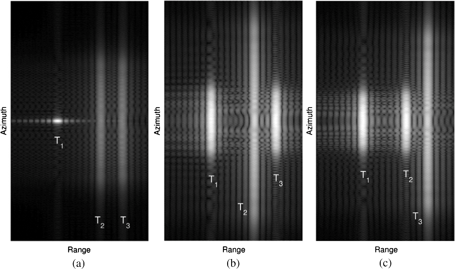$H_{2} (u)$ .

The azimuth velocity components of the three detected scatterers are estimated according to Eq. (22) by using the optical processor. The measured sharpness difference curves varying with $V_{a}^{'}$ are presented in Fig. 5. In the estimation process, $V_{a}^{'}$ ranges from 0 to $20 m / s$ with regular increments of $0.5 m / s$ . The sharpness difference curve of $T_{1}$ is flat because a stationary target tends to be defocused to the same extent in the SLMs $M_{2}$ and $M_{3}$ . The sharpness difference curve of $T_{2}$ reaches its valley value at $V_{a}^{'} = 10 m / s$ , and it indicates that the target’s azimuth velocity is $- 10 m / s$ . The sharpness difference curve of $T_{3}$ reaches its peak value at $V_{a}^{'} = 10 m / s$ , and it indicates that the azimuth velocity of $T_{3}$ is $10 m / s$ . From Fig. 5 we see that the maximum sharpness difference values appear at the expected azimuth velocity points. The simulation results show that the proposed scheme is feasible and effective.

Fig. 5

Sharpness difference curves of the three simulated targets.

During our simulations, we find that the scheme provides high measurement precision because of the sharp and high sharpness difference curve for a large azimuth velocity, while for a small azimuth velocity, the measurement precision is poor because its sharpness difference curve is fairly flat and low.

4.2.

Field Data

A set of field SAR data is used to verify the optical processor. Figure 6(a) shows an image of two vehicles moving along a runway at the speed of $5 m / s$ in the same direction. The targets are labeled by $T_{1}$ and $T_{2}$ , respectively. The radar waveform parameters are listed as follows. The carrier frequency is 9.6 GHz, the pulse width is 20 μs, the bandwidth is 400 MHz, and the pulse repetition frequency is 1200 MHz. The platform moves at the speed of $218 m / s$ along the runway. From Fig. 6(a) we see that the images of the two vehicles are smeared in the azimuth direction.

Fig. 6

Experimental results of field data. (a) A field SAR image patch. (b) Defocused image by $H_{1} (u)$ . (c) Defocused image by 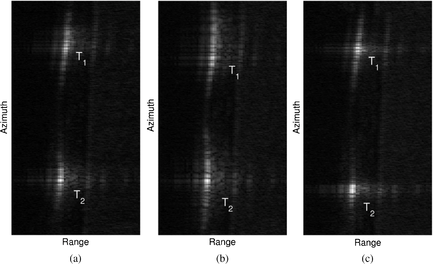$H_{2} (u)$ .

In the target detection process, the SLMs $M_{2}$ and $M_{3}$ are modulated by $H_{1} (u)$ and $H_{2} (u)$ with $ε_{a}^{'} = 0.029$ ( $V_{a}^{'} = 5 m / s$ ), respectively. After being filtered by $M_{2}$ and $M_{3}$ , two defocused SAR images are generated and shown in Fig. 6(b) and 6(c), respectively. It can be seen that the two vehicles are smeared even worse in Fig. 6(b) and focused better in Fig. 6(c). By computing the sharpness difference of the two defocused images, the moving vehicles can be indicated.

The azimuth velocity components of the two detected vehicles are measured according to Eq. (22) by using the proposed optical processor. The measured sharpness difference curves varying with $V_{a}^{'}$ are presented in Fig. 7. In the estimation process, $V_{a}^{'}$ ranges from 0 to $10 m / s$ with regular increments of $0.5 m / s$ . The two curves reach their valley values at $V_{a}^{'} = 5 m / s$ approximately. It indicates that the speed of the vehicles is about $- 5 m / s$ .

Fig. 7

Sharpness difference curves of the two targets in the field data. (a) Sharpness difference of $T_{1}$ . (b) Sharpness difference of $T_{2}$ .

The curves in Fig. 7 show a nonmonotonic behavior due to the radar imaging process. Uncontrollable measurement conditions, such as the vibration of antenna, nonstraight trajectory of the platform, external interference, and digitalization, will cause phase errors in the echoes during the signal collection process. So there are some subtle differences between the two defocused images of the background, which is mixed in the detected moving target. As a result, the sharpness difference curve of a real moving target appears uneven. However, the trends of the two curves in Fig. 7 are similar to that in Fig. 2. This experimental result shows that the proposed scheme can deal with the field data practically.

5. Conclusion

In summary, we have presented an optical MTI to detect moving targets and estimate their azimuth velocities in SAR images. In principle, it is robust against clutter and interference. The experimental results using both simulated and field data show that the proposed optical architecture is feasible, effective, and practical.

Acknowledgments

We appreciate the support from the Shandong Young Scientists Award Foundation (Grant Number: BS2010DX021) and the National Natural Science Foundation of China (Grant Number: 61070175 and 61175053).

References

1.

R. Raney, “Synthetic aperture imaging radar and moving targets,” IEEE Trans. Aerosp. Electron. Syst., AES-7 (3), 499 –505 (1971). http://dx.doi.org/10.1109/TAES.1971.310292 IEARAX 0018-9251 Google Scholar

2.

J. Fienup, “Detecting moving targets in SAR imagery by focusing,” IEEE Trans. Aerosp. Electron. Syst., 37 (3), 794 –809 (2001). http://dx.doi.org/10.1109/7.953237 IEARAX 0018-9251 Google Scholar

3.

J. WangX. Liu, “Velocity estimation of moving targets using SAR,” in Proc. IEEE IGARSS, 340 –343 (2011). Google Scholar

4.

P. MarquesJ. Dias, “Moving targets processing in SAR spatial domain,” IEEE Trans. Aerosp. Electron. Syst., 43 (3), 864 –874 (2007). http://dx.doi.org/10.1109/TAES.2007.4383579 IEARAX 0018-9251 Google Scholar

5.

D. Weihinget al., “Detection of along-track ground moving targets in high resolution spaceborne SAR images,” ISPRS J. Photogramm. Remote Sens., 61 (3–4), 135 –140 (2006). http://dx.doi.org/10.1016/j.isprsjprs.2006.09.011 IRSEE9 0924-2716 Google Scholar

6.

R. Bamler, “Doppler frequency estimation and the Cramer-Rao bound,” IEEE Trans. Geosci. Remote. Sens., 29 (3), 385 –390 (1991). http://dx.doi.org/10.1109/36.79429 IGRSD2 0196-2892 Google Scholar

7.

I. CummingS. Li, “Improved slope estimation for SAR Doppler ambiguity resolution,” IEEE Trans. Geosci. Remote. Sens., 44 (3), 707 –718 (2006). http://dx.doi.org/10.1109/TGRS.2005.861925 IGRSD2 0196-2892 Google Scholar

8.

F. McFadden, “Precise pose estimation for synthetic aperture radar images of vehicles,” Opt. Eng., 46 (10), 107201 (2007). http://dx.doi.org/10.1117/1.2793710 OPEGAR 0091-3286 Google Scholar

9.

D. PsaltisK. Wagner, “Real-time optical synthetic aperture radar (SAR) processor,” Opt. Eng., 21 (5), 822 –828 (1982). http://dx.doi.org/10.1117/12.7972988 OPEGAR 0091-3286 Google Scholar

10.

F. DickeyJ. Mason, “Optical Synthetic-aperture radar processor architecture with quadratic phase-error correction,” Opt. Lett., 15 (20), 1162 –1164 (1990). http://dx.doi.org/10.1364/OL.15.001162 OPLEDP 0146-9592 Google Scholar

11.

B. Wang, Digital Signal Processing Techniques and Applications in Radar Image Processing, 254 –255 Wiley, Hoboken, NJ (2008). Google Scholar

12.

J. Fienup, “SAR autofocus by maximizing sharpness,” Opt. Lett., 25 (4), 221 –223 (2000). http://dx.doi.org/10.1364/OL.25.000221 OPLEDP 0146-9592 Google Scholar

Biography

Yuan Li received her BSc degree from the Qufu Normal University, Shandong, China, in 1998, a MSc degree from University of Electronic Science and Technology of China, Sichuan, China, in 2001 and a PhD degree from the Chinese Academy of Engineering Physics (CAEP), Beijing, China, in 2007. From 2007 to 2010, she was an engineer with IEE of CAEP, Mianyang, China, where she worked on signal processing and ISAR systems. She is currently a teacher in Shandong Institute of Business and Technology, and a researcher in the Key Laboratory of Intelligent Information Processing in Universities of Shandong, Yantai, China. Her research interests include coherent optical signal processing, radar signal processing, and ground moving target indication.

Gaohuan Lv received his BSc degree from the Qufu Normal University, Shandong, China, in 1998, a MSc degree from the Chinese Academy of Engineering Physics, Beijing, China, in 2001 and a PhD degree from the Shanghai Jiao Tong University, Shanghai, China, in 2013. From 2001 to 2008, he was an engineer with IEE of CAEP, Mianyang, China, where he worked on control system and software engineering. His research interests include coherent optical signal processing, radar signal processing, digital image processing, and ground moving target indication.

CC BY: © The Authors. Published by SPIE under a Creative Commons Attribution 4.0 Unported License. Distribution or reproduction of this work in whole or in part requires full attribution of the original publication, including its DOI.

Citation Download Citation

Yuan Li and Gaohuan Lv "Optical moving target indicator for synthetic aperture radar images," Optical Engineering 52(8), 083103 (2 August 2013). https://doi.org/10.1117/1.OE.52.8.083103

Published: 2 August 2013

Access the abstract

JOURNAL ARTICLE
8 PAGES

DOWNLOAD PAPER SAVE TO MY LIBRARY

GET CITATION

KEYWORDS

Synthetic aperture radar

Target detection

Doppler effect

Spatial light modulators

Computer architecture

Image filtering

Modulation

1.

Introduction

2.

Principles

2.1.

Moving Target Detection in Space Domain

Eq. (1)

Eq. (2)

Eq. (3)

Eq. (4)

Eq. (5)

Eq. (6)

Eq. (7)

Eq. (8)

Eq. (9)

Eq. (10)

Fig. 1

Eq. (11)

Eq. (12)

Eq. (13)

Eq. (14)

Eq. (15)

Eq. (16)

Eq. (17)

Eq. (18)

Eq. (19)

2.2.

Azimuth Velocity Component Measurement

Eq. (20)

Eq. (21)

Eq. (22)

Eq. (23)

Eq. (24)

Fig. 2

3.

Implementation

Eq. (25)

Fig. 3

4.

Results

4.1.

Computer Simulation

Fig. 4

Fig. 5

4.2.

Field Data

Fig. 6

Fig. 7

5.

Conclusion

Acknowledgments

References

Biography

Show All Keywords

Keywords/Phrases

Search In:

Publication Years