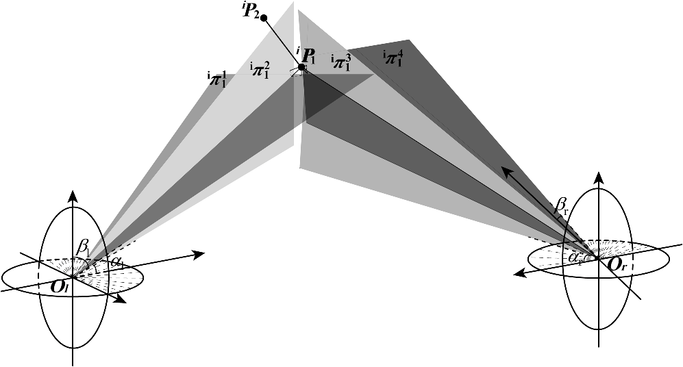
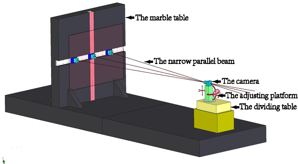
1.

Introduction

Stereoscopic system is considered a classic system in photography measurement. Accurate calibration of cameras is especially crucial, because it plays an important role in the measurement accuracy of a stereoscopic system. General calibration of a stereoscopic system consists of estimating the internal and external parameters. The internal parameters determine the image coordinates of the measured points in a scene with respect to the camera coordinate frame, and the external parameters represent the geometrical relationship between the camera and the scene or between the different cameras.

The existing techniques for camera calibration can be classified into two categories: parametric methods and general nonparametric methods.¹

Parametric calibration methods are standard approaches to discover the relation of the three-dimensional (3-D) Euclidean world to the two-dimensional image space. However, for each different sensor type, a different parametric representation is required. In photography measurement, pinhole cameras are often used, so we mainly review the works that have been done for regular pinhole cameras.

Considering all the parameters simultaneously, a direct nonlinear minimization is a good choice by using an iterative algorithm with the objective of minimizing residual errors of some equations.^2,3 The great disadvantage is that the nonlinear processing may end in a local solution with different types of parameters included in one space. Some existing linear methods solve linear equations established by some constraints with the goal of computing a set of intermediate parameters.^4,5 But in most cases, the lens distortions are not considered so the accuracy of the final solution is relatively low. Other parametric methods may compute some parameters first and then followed by others. Tsai⁶ derived a closed form solution for external parameters and the focal length and then used an iterative scheme to estimate other parameters. Straight lines in space were used as constraints in order to find the right parameters of the distortion model in Refs. 7–9. In Ref. 10, geometrical and epipolar constraints were imposed in a nonlinear minimization problem to correct points’ location in images first and then the lens distortion and fundamental matrix were estimated separately.

With the parameterized model to handle the lens distortion, we find a serious discrepancy that the results obtained with calibration data are better than the ones with testing data.¹¹ This discrepancy can be explained by the inadequacy of the parameterized distortion model.

An alternative idea of nonparametric camera calibration was introduced by Grossberg and Nayar,¹² who used a set of virtual sensing elements called raxels to describe a mapping from incoming scene rays to photosensitive elements on the image detector, and a more general approach was developed in Refs. 1314.–15. In this generic method, several planar calibration objects are used to determine the corresponding optical ray of each pixel, and it is powerful as it can be applied equally well to any arbitrary imaging systems. But for close-range photogrammetry, the calibration from pixel to pixel does not realize high-accuracy measurements.

We have designed a pure optical distortion correction method for calibrating perspective imaging systems. The proposed method inherits the idea of nonparametric modeling and uses precise rotating platform and subpixel image processing to realize the mapping between incoming scene rays and photosensitive elements on the image detector (every photosensitive element could be divided into many parts to improve the accuracy if necessary). Then, we applied it to the calibration of a stereo vision system. In contrast to the standard parametric approach, it decouples the distortion estimation from the calibration of external parameters of two cameras at the same time, thus avoiding any error compensation between each other.^16,17

2.

Proposed Camera Correction Process

In the pin-hole camera model, the object point in scene and its image point obey a certain geometrical constraint: object point $P$, image point $p$, and the optical center of camera $O$ lie in a line.

Because of the distortion in real circumstances, the optical lines are refracted when passing through the optical center. Then, we obtain the distorted image points that have deviations from the ideal ones. The parametric methods try to establish mathematical models in order to relate the distorted image plane and the undistorted one correctly. But, apparently, it is difficult since the distortion caused by the lenses shows both regularity and irregularity.

So, we proposed a pure optical correction method to record the rays entering into the lens, as many as possible. Every ray will have an image when entering into lenses, and the direct method is to relate the coordinate of the image point and the angle determining the incident ray.

First, we establish a Cartesian coordinate system as shown in Fig. 1. Take the optical center as origin $O$, optical axis as $Z$-axis, and make $X$-axis and $Y$-axis parallel to the vertical and horizontal axes of image plane, respectively. Then, rotate the camera around $X$-axis and take a photograph of a fixed straight line in scene at every certain interval. At every angle ${\alpha }_i$ that determines the plane ${\pi }_i$, we can get the distorted image $l_i$ of the straight line $L_i$ on the image detector. When all of the angles in the field of view are recorded, a database about one-to-one correspondence between the angle ${\alpha }_i$ and the curved line $l_i$ has been already established. Then, rotating the camera for 90 deg around $Z$-axis, with the same method, we can get another angle ${\beta }_i$.

Fig. 1

A schematic diagram of the pure optical correction method. In practice, the straight line was composed of many points, and there were many rotating angles, so at $i$’th rotation, denotes ${\alpha }_i$ and $l_i$ as the corresponding angle and image (composed of image points) of the straight line, respectively.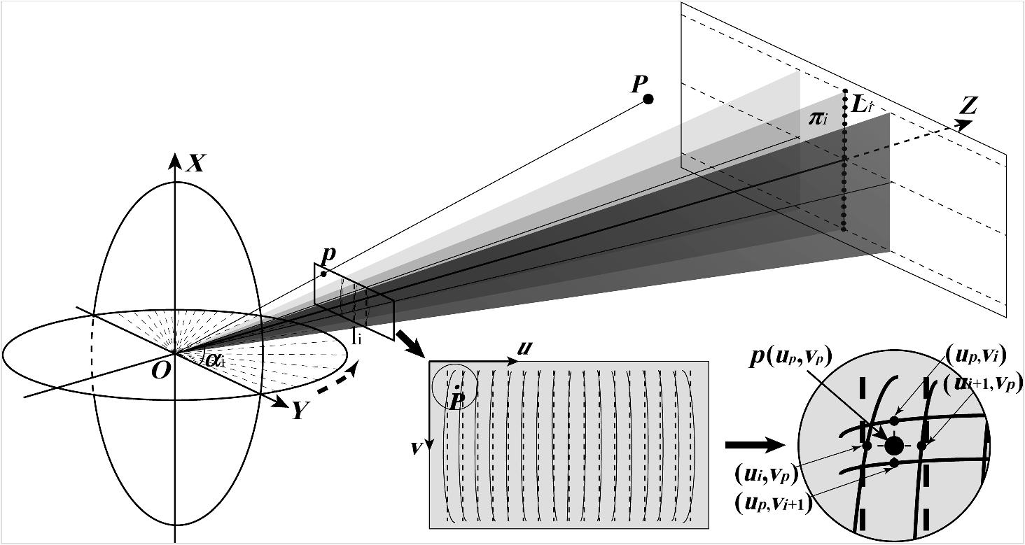

Since, in practice, not all the incident rays could be recorded, the image plane is divided into many square grids. If the interval of the rotating angle is set small enough, high-accuracy results can be obtained. Given an arbitrary point $P$ in measuring field, as shown in Fig. 1, its correspondence on the image plane will lie in a small grid. We can get the fitted angle by bilinear interpolation¹⁸ as

So with any measured point’s image coordinate $(u,v)$, we can calculate its corresponding angle $(\alpha ,\beta )$. If the image point just lies on the curved line, we can directly get the corresponding angle through searching the database.

3.

Calibration of a Stereoscopic System

When the above-mentioned procedures are completed, the stereoscopic system can be easily calibrated by placing a fixed-length reference one-dimensional (1-D) target arbitrarily in the field of view, which is commonly used.^3,19 As shown in Fig. 2, two feature points are fixed on the ends of reference target with the distance exactly known in advance.

Fig. 2

One-dimensional target and the feature points were marked by a red circle and magnified to show more details.

The external parameters of a stereoscopic system include rotation matrix $R$ and translation vector $T$, which can be represented with the essential matrix $E$. Let $F$ be the fundamental matrix of a stereoscopic system, then we have

The fundamental matrix can be computed with the eight-point algorithm proposed in Refs. 4 and 20. At least seven pairs of corresponding virtual image points and the distance $L$ are needed to obtain $R$, $T$, and the 3-D coordinates of the reconstructed feature points, which are used as the initial values of the following nonlinear minimization.

Then, we can establish the minimization function to obtain optimal values of external parameters with the fixed length of 1-D target and geometrical constraints.

As shown in Fig. 3, ${{}^{i}P}_1$, and ${{}^{i}P}_2$ represent two feature points located in the 1-D target, where $i$ is the number of positions that the 1-D target has been placed in. The plane, that ${{}^{i}P}_1$ should lie on, is ${{}^i\pi }_1^j$, where $j$ is the number of the plane since a feature point is the intersection point of four planes; $d(,)$ represents the distance between a point and a plane. Then, we have the error equation as follows:

Fig. 3

A schematic diagram of the constraints of optical planes.

Denote $L$ and $D(,)$ as the true and measured distance between the two feature points of the 1-D target, respectively, then we have

With Eqs. (3) and (4), the minimization equation is established as follows:

The nonlinear minimization has the angles to feature points from the optical center and the real length of 1-D target as inputs. External parameters $X$ and feature points $P$ are corrected to minimize Eq. (5). The algorithm is a Levenberg–Marquardt nonlinear minimization that starts with the initial values $X_0$ and $P_0$ and ends with the optimized solution of the external parameters.

4.

Experiments

4.1.

Optical Correction for the Camera

A pure optical method requires a high-accuracy straight line in scene which can be captured by the camera. Note that the subpixel detection of image dots gives more reliable results than cross detection.²¹ A photoreflector material seems like a good choice, but it is liable to be affected by lighting variation, and an extra light source is often needed to get high contrast ratio. Since the repetitive positioning accuracy of the light-emitting diode’s (LED) image is better than 0.02 pixels,^22–24 a set of near-infrared LEDs were used, which were adjusted into a straight line by a high-accuracy linear guide.

The rotation of the camera around an axis was completed by the multitooth dividing table. The determination of the optical center that must be coincident with the rotating axis of multitooth-dividing table is critical to the overall accuracy. The determination of the rotating axis was completed by a six-dimensional (6-D) high-accuracy adjustable platform, a physical axis, and a dial gauge, as shown in Fig. 4. The multitooth-dividing table can rotate 360 deg. We adjusted the 6-D high-accuracy adjustable platform to keep numerical values measured by the dial gauge almost invariant when the multitooth-dividing table was rotating.

Fig. 4

The procedures of determining the rotating axis by a six-dimensional (6-D) precision adjustable platform, a physical axis, and a dial gauge.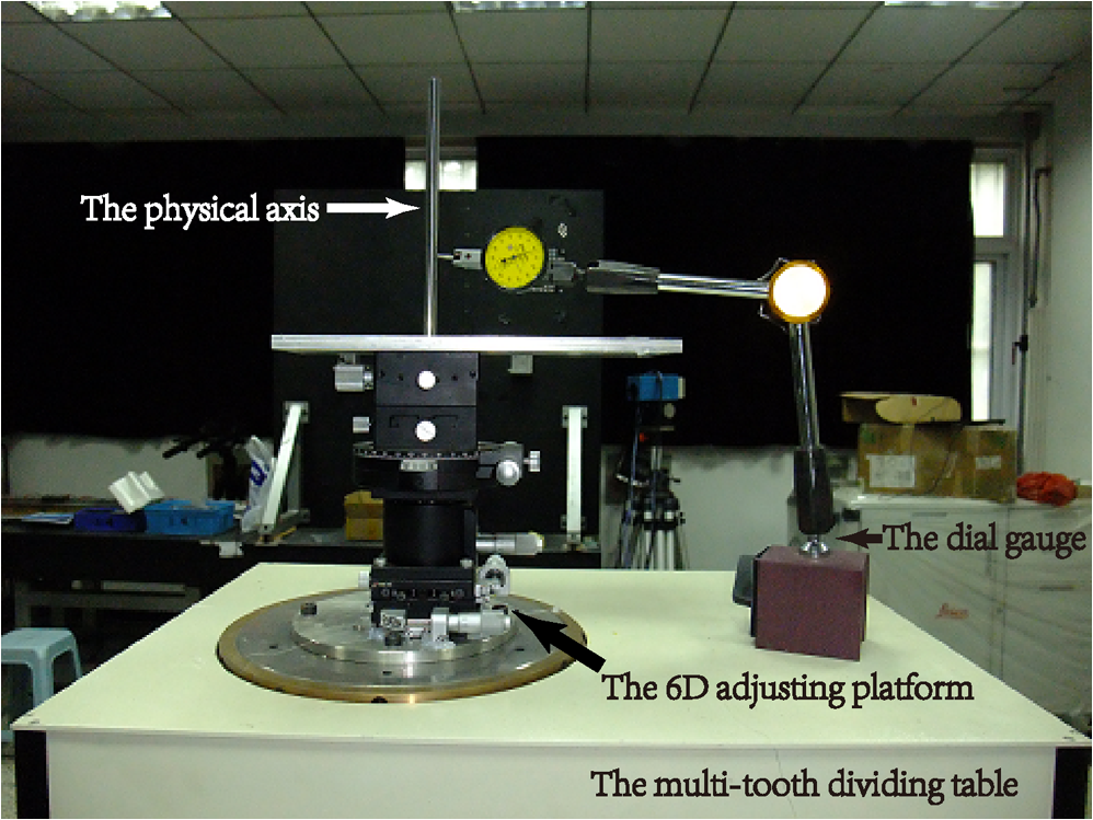

We used collimated semiconductor laser beams shaped by an aperture stop as the narrow parallel beams, and in space we need at least two beams to determine a point. Here, we used three beams as shown in Fig. 5.

Fig. 5

Align the optical center with the rotating axis using three beams.

The process of the alignment of the optical center with the rotating axis was

• 1. As shown in Fig. 4, make the rotating axis coincide with the physical axis to visualize the rotating axis;

• 2. Adjust three beams to meet at a point right on the physical axis;

• 3. Replace the physical axis with a camera and adjust the 6-D high-accuracy adjustable platform to make the three beams pass through the optical center, as shown in Fig. 5;

• 4. Use a multitooth-dividing table to control the rotation angles of the camera precisely. For the multitooth-dividing table, the minimum rotation interval is 1 arc sec and rotation accuracy is 0.6 arc sec.

To test the performance of the pure optical method, a corrected camera was placed at several locations to capture multiple images of the straight line which was composed of a set of feature points before the camera. With the image coordinates of the feature points, we could obtain the corresponding horizontal and vertical angles through the proposed method, and all the feature points were reprojected on a virtual image plane, which was perpendicular to the optical axis. Then, their regression line was computed and the root mean square (RMS) distance from each feature point to the line was used as the measure error.

Figure 6 denotes the orientation of the lines on the virtual image plane corrected by our method and Table 1 shows the RMS errors of the corrected and uncorrected lines, from which we can see that the RMS errors (in pixels) of the feature points to their regression lines were improved with our method.

Fig. 6

The line composed of near-infrared LEDs (a) were captured by camera in six orientations as shown in (b).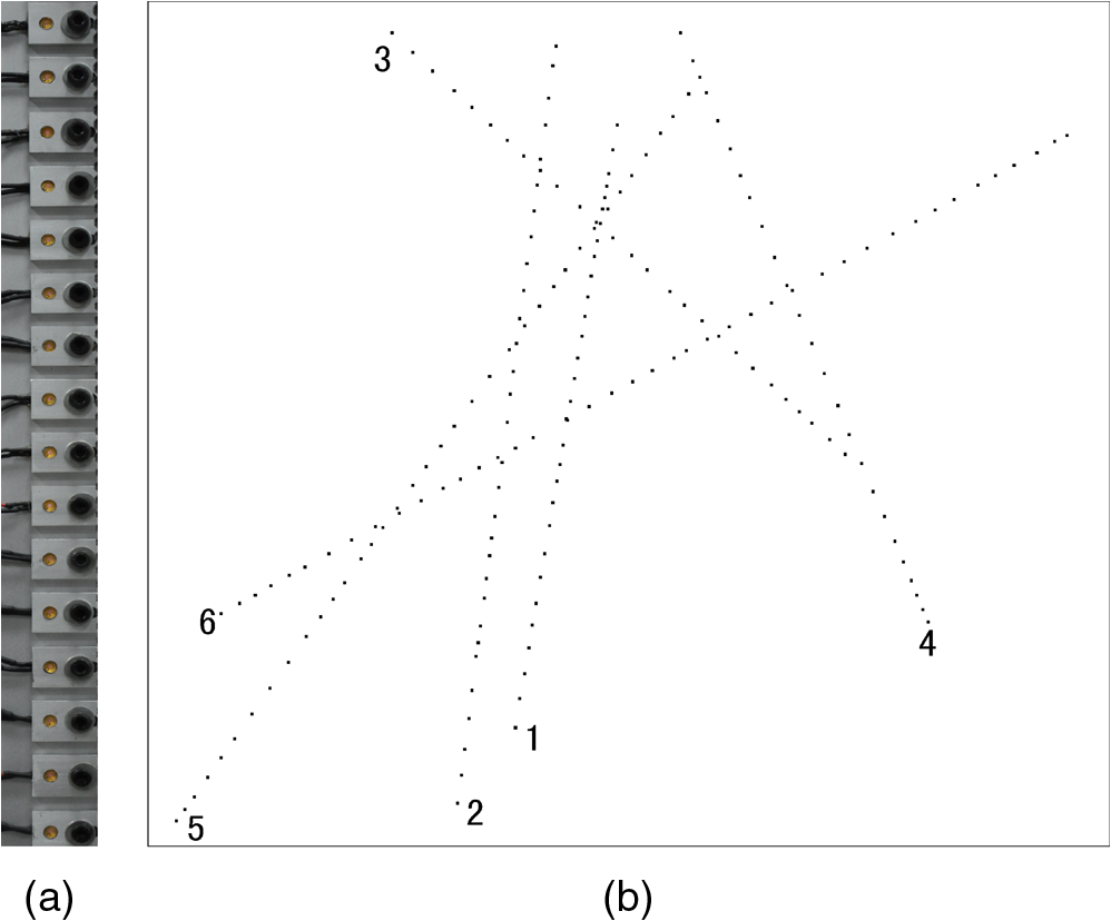

Table 1

The root mean square error (RMSE, in pixels) of the feature points to their regression lines.

RMSE (in pixels)
	Corrected by our method	Uncorrected
Line 1	0.0535	0.0666
Line 2	0.1007	0.1062
Line 3	0.0644	0.1637
Line 4	0.1033	0.1763
Line 5	0.1099	0.2034
Line 6	0.0771	0.2371

5.

Conclusion

A novel camera calibration method based on nonparametric models has been defined. First, a database has been obtained to remove influences of the distortion caused by lenses by a pure optical adjustment method. Second, a stereoscopic system has been established to test the performance of the proposed method, and the external parameters of cameras can be accurately acquired with the 1-D target. This method gets rid of the constraints of camera distortion models, and it is applicable to a central camera equipped with any lenses. Also, the coupling among all the intrinsic and external parameters is avoided, which may otherwise lead to instability and compensation of each other. On the other hand, as the subdivision number of angles increases, the correction time increases too. However, since camera correction is an off-line process, more time consumed for higher accuracy is acceptable.