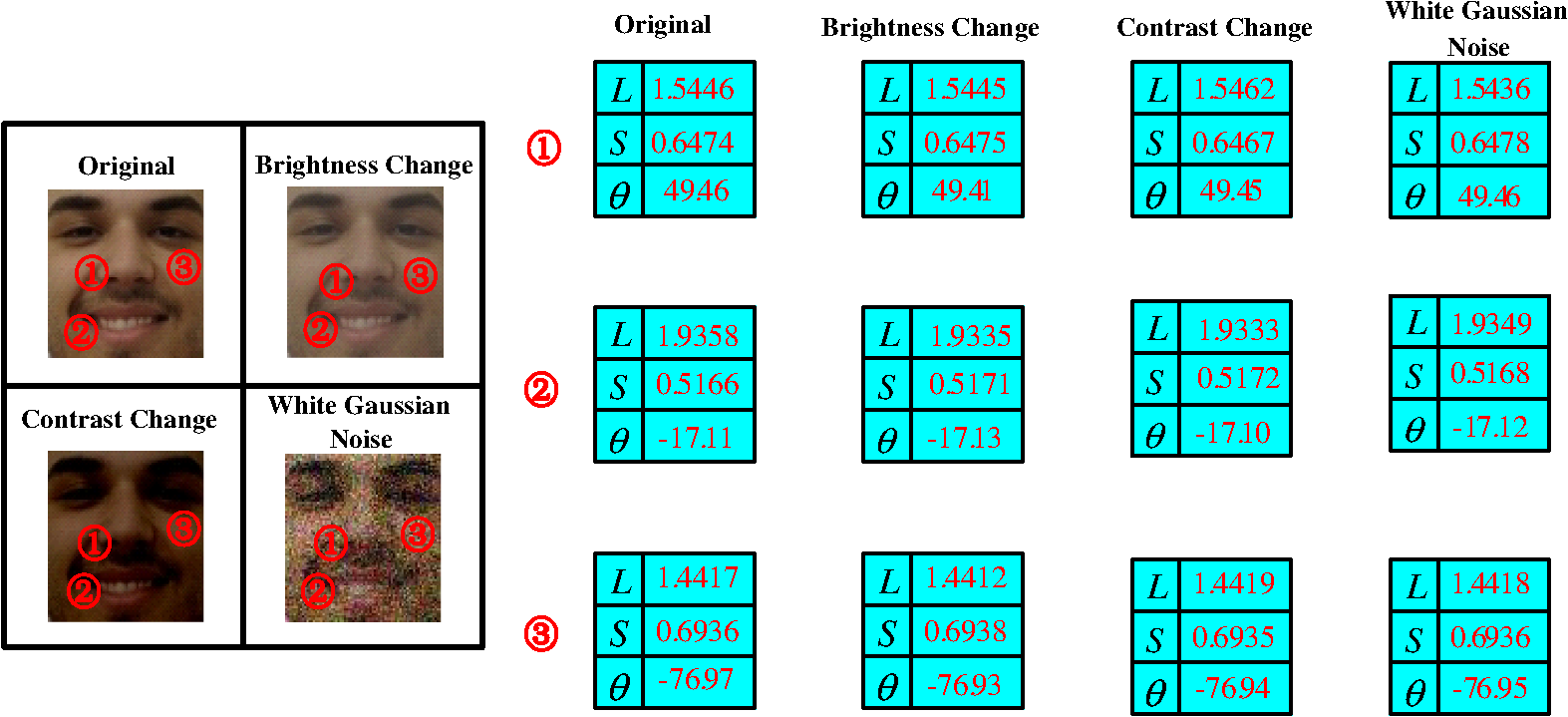
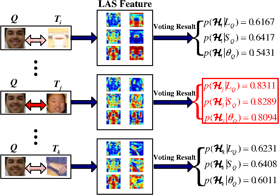
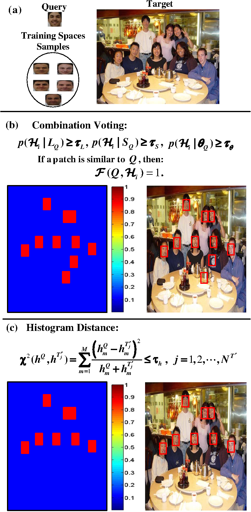
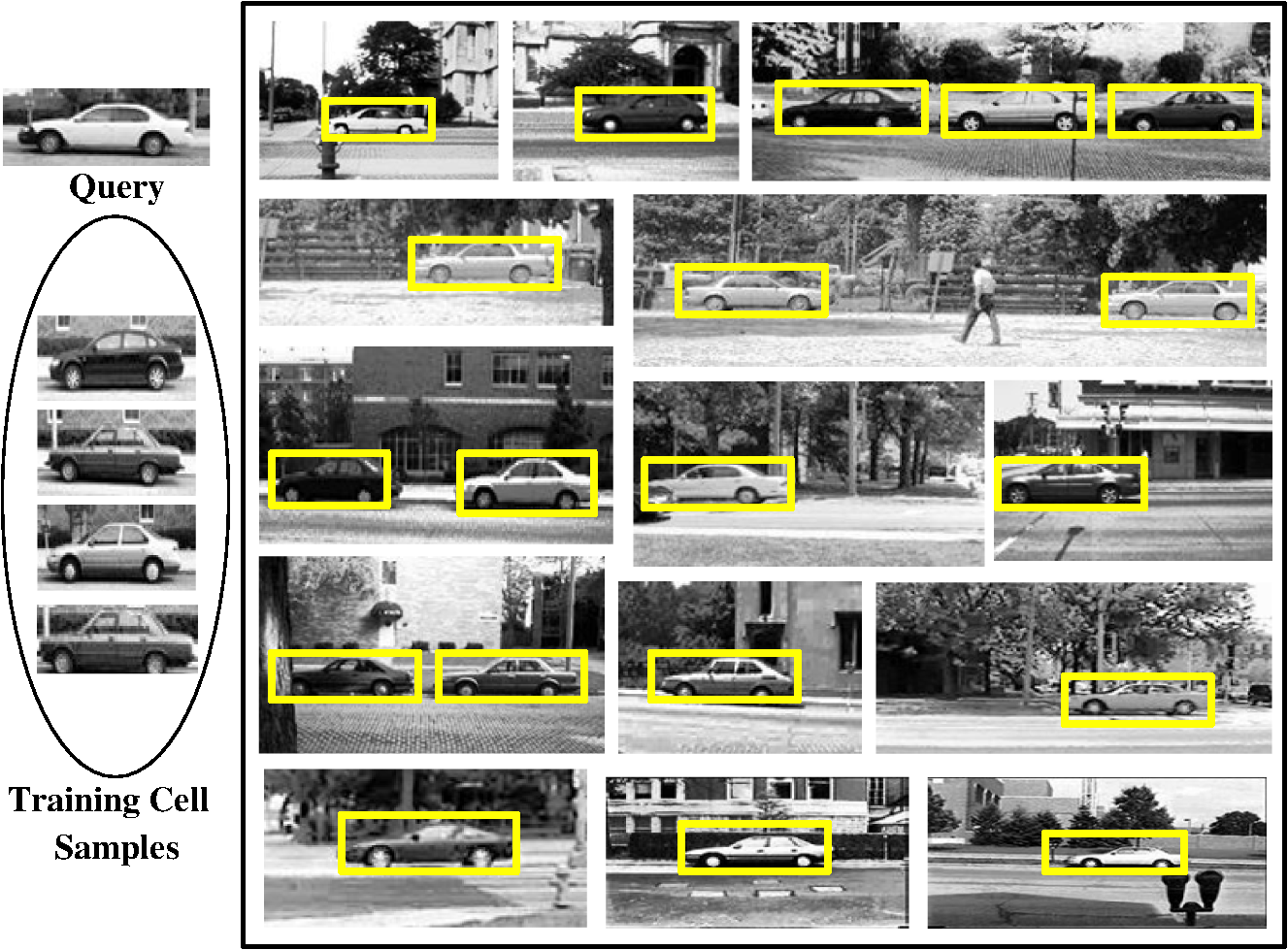
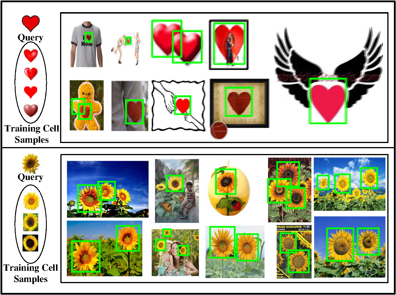
1.

Introduction

Object detection from a target image has attracted increasing research attention because of a wide range of emerging new applications, such as those on smart mobile phones. Traditionally, pattern recognition methods are used to train a classifier with a large number, possibly thousands, of image samples.^1–10 An object in a sample image is a composite of many visual patches or parts recognized by some sparse feature analysis methods. In the detection process, sparse features are to be extracted in a testing image and a trained classifier is used to locate objects in a testing image. Unfortunately, in most real applications there are always insufficient training samples for robust object detection. Most likely, we may just have a few samples about the object we are interested in, such as the situations in passport control at airports, image retrieval from the Web, and object detection from video or images without preprocessed indexes. In these cases, the template matching approach based on a small number of samples often has been used.

Designing a robust template matching method remains a significant effort.¹¹ Most template matching approaches use query image to locate instances of the object by densely sampling local features. Shechtman and Irani provided a single-sample method¹² that uses a template image to find instances of the template in a target image (or a video). The similarity between the template and a target patch is computed by a local self-similarity descriptor. In Refs. 13 and 14, one sample, representing human behavior or action, is used to query videos. Based on this training-free idea, Seo and Milanfar proposed the locally adaptive regression kernels (LARK) feature as the descriptor to match with the object in a target image using only one template.¹⁵ This LARK feature, which is constructed by local kernels, is robust and stable, but this LARK feature brings overfitting problem and results in low computational efficiency.In Ref. 16, the authors constructed an inverted location index (ILI) strategy to detect the instance of an object class in a target image or video. This ILI structure saves the feature locations of one sample and indexes feature values according to the locations to locate the object in target image. But this ILI structure just processes one sample. In order to improve the efficiency and accuracy based on a small number of training samples, these methods have to run a few times on each of those samples.

Different from the dense feature like LARK, key-point sampled local features, such as scale invariant feature transform (SIFT)¹⁷ and speeded up robust features (SURF),¹⁸ always obtain a good performance in the case of using thousands of samples to train classifiers. And these key-point features are always in a high-dimensional feature space. If one has thousands of samples and needs to learn classifiers such as support vector machine (SVM),^3,8 key-point features have obtained good performance. Previous works^15,19–21 pointed out that the densely sampled local features always give better results in classification tasks than that of key-point sampled local features like SIFT¹⁷ and SURF.¹⁸

Recently, some interesting researches based on few samples have emerged. Pishchulin et al. proposed a person detection model from a few training samples.²² Their work employs a rendering-based reshaping method in order to generate thousands of synthetic training samples from only a few persons and views. However, the samples are not well organized and their method is not applicable on generic object detection. In Ref. 23, a new object detection model is proposed named the fan shape model (FSM). FSM uses a few samples very efficiently, which handles some of the samples to train out the tolerance of object shape and makes one sample the template. However, FSM method is not scalable in terms of samples and is only for contour matching.

In this paper, we propose a novel approach for generic object detection based on few samples. First, a new type of feature at each pixel is considered, called locally adaptive steering (LAS) feature, which is designed for a majority voting strategy. The LAS feature at 1 pixel can describe the local gradient information in the neighborhood, which consists of the dominant orientation energy, the orthogonal dominant orientation energy, and the dominant orientation angle. Then, for each member of this feature, a cell is constructed at each pixel of the template image, whose length is the range of the feature member value. The cells for all pixels construct a voting space. Since this feature is in three dimensions, three voting spaces are to be constructed. We use a few samples to train these voting spaces, which represent the tolerance of appearance of an object class at each pixel location.

Our idea of using a LAS feature is motivated by earlier work on adaptive kernel regression²⁴ and the work of LARK feature.¹⁵ In Ref. 24, to perform denoising, interpolating, and deblurring efficiently, localized nonlinear filters are derived that adapt themselves to the underlying local structure of the image. LARK feature can describe the local structure very well. After densely extracting LARK features from template and target images, matrix cosine similarity is used to measure the similarity between query image and a patch from target image. This method is resilient to noises and distortions, but the computation of LARK features is time-consuming with heavy memory usage. Our LAS feature simplifies the computation of LARK and saves the memory. Moreover, LAS feature also exactly captures the local structure of a specific object class.

Our voting strategy is inspired by the technology of Hough transformation. Many works^25–30 have contributed to model spatial information at locations of local features or parts as opposite to the object center by Hough voting. The Hough paradigm starts with feature extraction and each feature casts votes for possible object positions.⁴ There are two differences from Hough voting. The first one is each cell size of the voting spaces is trained out by samples. But each cell size of the Hough voting space is all fixed. Our trained space can tolerate more deformation. The second one is our voting strategy is based on template matching. Previous Hough voting is based on a trained code-book with thousands of samples.

This paper is structured as follows. Section 2 gives an overview of our method. In Sec. 3, we propose LAS feature. Section 4 describes the concept of voting space and the training processing. Section 5 introduces the procedure of object matching in voting spaces. Section 6 gives the experimental results and compares our method with the state-of-the-art methods. This paper is extended from an early conference paper³¹ with improved algorithms and comprehensive experimental results.

2.

Overview of Our Approach

An overview of our method is shown in Fig. 1. In the training processing, for each dimension of LAS feature, a voting space is constructed by image coordinates $(x,y)$ and corresponding value ranges of the feature member. Each cell in the voting space is formed by the corresponding pixel position and its value range of this feature member, which is trained by several samples. Since the voting space is three dimensional (3-D), for simplicity we use a 3-D box to represent a cell. The longer the box is, the higher the cell length. The different sizes of boxes mean the different tolerances of object appearance changes at corresponding pixels. In Fig. 1, LAS feature $(L,S,\theta )$ is specially designed for object matching in voting spaces, where $L$, $S$, and $\theta$ represent the dominant orientation energy, the orthogonal dominant orientation energy, and the dominant orientation angle, respectively, in the neighborhood at each location. Thanks to the merit of voting, only a few samples (2 to 10 samples in this paper) are enough to train cells.

Fig. 1

The overview of our method. In the trained voting spaces, $(x,y)$ means the query image coordinates. Each bin in the spaces is corresponding to the pixel cell.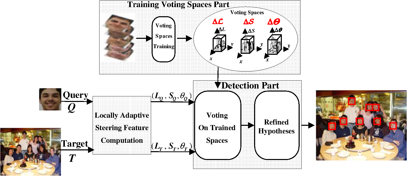

In the detection process, by randomly choosing one sample image as the query $Q$, the instances of an object class are located in target image $T$, which is always larger than $Q$. First, the patches $T_i$ extracted from $T$ by a sliding window are detected by densely voting in the trained voting spaces. Each component of LAS feature of $T_i$ and $Q$ is voted in each voting space to obtain a value of similarity. If the values of similarity of all LAS features are larger than the corresponding thresholds, then $T_i$ is a similar patch of $Q$. Then a refined hypotheses step is used to accurately locate the multiple instances by computing the histogram distance corresponding to the feature $\theta$. The refined step is just processing the similar patches that are obtained in the voting step. If the histogram distance of $\theta$ between a similar patch and $Q$ is small enough, then the similar patch is the object instance.

3.

Locally Adaptive Steering Feature

The basic idea of our LAS is to obtain the locally dominant gradient orientation of image. For gray image, we compute the gradient directly. If the image is RGB, the locally dominant gradient orientation is almost the same on each channel. To reduce the computation cost of transforming RGB to gray image, we just use the first channel of RGB. The dominant orientation of the local gradient field is the singular vector corresponding to the smallest singular value of the local gradient matrix.^24,32 (The proof of transformation invariance of singular value decomposition (SVD) can be reviewed by interested readers from Ref. 24.) For each pixel $(i,j)$, one can get the local gradient field shown in Fig. 2(a). The local gradient field is a patch in the gradient map around the pixel $(i,j)$. Here, the size is set as $3\times 3\text{pixels}$. The dominant orientation means the principal gradient orientation in this gradient field. To estimate the dominant orientation, we compute the horizontal and orthogonal gradients of the image. Then, the matrix $GF(i,j)$ is concatenated column-like as follows:

Fig. 2

(a) Locally adaptive steering (LAS) feature at some pixels. The red dots mean the positions of pixels. The ellipse means the dominant orientation in the local gradient patch around the corresponding pixel. (b) The components of LAS feature in an image. $L$, $S$, and $\theta$ are shown as a matrix, respectively.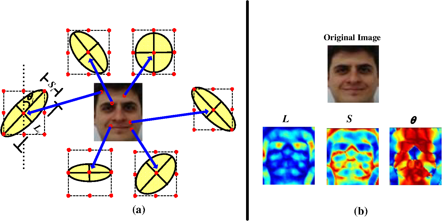

The eigenvalues ${\lambda }_1$ and ${\lambda }_2$ represent the gradient energies on the principal and minor directions, respectively. Our LAS feature at each pixel is denoted as $(L_{(i,j)},S_{(i,j)},{\theta }_{(i,j)})$. We define a measure $L_{(i,j)}$ to describe the dominant orientation energy as follows:

The measure ${\theta }_{(i,j)}$ is the rotation angle of $L_{(i,j)}$, which represents the dominant orientation angle.

The LAS feature can describe the local gradient distribution information (see Fig. 2). $L$, $S$, and $\theta$ are from the computation of the local gradient field, which can yield invariance to brightness change, contrast change, and white noise as shown in Fig. 3. The results of Fig. 3 are from the computation of LAS feature under different corresponding conditions. Due to the SVD decomposition of local gradients, the conditions of Fig. 3 on each pixel do not change the dominant orientation energy enormously. One can find the proof details of the tolerance of white noises, brightness change, and contrast change from Ref. 24.

Fig. 3

Robustness of the LAS feature in different conditions. The sigma of Gaussian noise is 4.

Some studies^15,19–21 have already pointed out that the densely sampled local features always give better results in classification tasks than that of key-point sampled local features, such as SIFT¹⁷ and SURF.¹⁸ These key-point sampled features are always in a high-dimensional feature space in which no dense clusters exist.¹⁵ Comparing to the histogram of gradient (HOG) feature,²⁷ our LAS feature has smaller memory usage. Each location of the HOG feature is 32 dimensions histogram, while our LAS feature is just three dimensions. In Ref. 33, the authors also proposed dominant orientation feature. But this dominant orientation is a set of representative bins of the HOG.³³ Our dominant gradient orientation is computed by the SVD decomposition of the local gradient values, which have more local shape information. Comparing to the LARK feature,¹⁵ our LAS feature has 27 times smaller memory usage, for the LARK feature is 81 dimensions at each pixel location. In Ref. 24, the authors mentioned these three parameters, but no one has used them as features. Next, we train the voting spaces based on this LAS feature to obtain three voting spaces.

So why can the LAS deal with only a few image samples well? That is because our LAS feature contains more local gradient information than other dense features like LARK¹⁵ and HOG.²⁷ There are three components of our LAS feature $L_{(i,j)}$, $S_{i,j}$, and ${\theta }_{i,j}$, which represent the dominant orientation energy, the orthogonal direction energy of dominant orientation, and the dominant orientation angle, respectively. For LARK,¹⁵ there is only gradient energy information, which cannot reflect the energy variations. For HOG,²⁷ there are just values of region gradient intensity in different gradient orientations, which cannot reflect dominant orientation energy and angle.

4.

Training Voting Spaces

The template image coordinates and the value ranges of the LAS feature component at the corresponding locations form the voting spaces (denoted as $\mathrm{\Delta }\mathcal{L}$, $\mathrm{\Delta }\mathcal{S}$, and $\mathrm{\Delta }\mathrm{\Theta }$, respectively, for three components of LAS feature). To match the template image and the patch from the target image (testing image) accurately, the cell length should be trained to reflect the tolerance of appearances at each pixel location. Several samples (2 to 10 samples in this paper) are enough to train the cells in each voting space.

Assume the query samples as $\mathcal{Q}=\{Q_1,Q_2,\dots ,Q_n\}$ and $n$ is the cardinality of $\mathcal{Q}$. We use Eqs. (3) to (5) to compute the LAS feature matrices of $n(n\ge 2)$ samples and obtain $\mathcal{L}=\{L^1,L^2,\dots ,L^n\}$, $\mathcal{S}=\{S^1,S^2,\dots ,S^n\}$, and $\mathrm{\Theta }=\{{\theta }^1,{\theta }^2,\dots ,{\theta }^n\}$. We want to get the tolerance at each location from the matrices $L^i$, $S^i$, and ${\theta }^i$ for ($i=1,2,\dots ,n$). Because our LAS feature is from local gradients at each location, each value in matrices $L^i$, $S^i$, and ${\theta }^i$ reflects the local edge orientation. To reflect the variation range of samples at each location, we define the cell sizes $\mathrm{\Delta }L$, $\mathrm{\Delta }S$, and $\mathrm{\Delta }\theta$ as follows:

Our definition of cell size is not the only choice. However, this definition is very simple and effective. Different from traditional training scheme, our training method, based on LAS feature, is not computationally expensive.

5.

Object Detection

A query image $Q$ is randomly selected from the sample images. And the target image $T$ is divided into a set of overlapping patches $\mathcal{T}=\{T_1,T_2,\cdots ,T_{N^T}\}$ by a sliding window with the same size as the query image $Q$, where $N^T$ is the number of patches in $\mathcal{T}$.

In our object matching scheme, there are two steps to search similar patches in $\mathcal{T}$. First step is voting in the trained voting spaces (see Fig. 5). To combine the votes from three voting spaces, we use a joint voting strategy to detect similar patches from $\mathcal{T}$. After the first step, one can get some similar patches ${\mathcal{T}}^{\prime }=\{T_1^{\prime },T_2^{\prime },\cdots ,T_{N^{T^{\prime }}}^{\prime }\}$ (${\mathcal{T}}^{\prime }\subset \mathcal{T}$ and $N_T^{\prime }$ is the cardinality of ${\mathcal{T}}^{\prime }$). Then a refined hypotheses step follows. In this step, the histogram distance of the LAS feature between $Q$ and $T_i^{\prime }(i=1,2,\cdots ,N^{T^{\prime }})$ is used to measure integral similarity, which can precisely locate the instances of the query $Q$.

5.1.

Voting in Trained Spaces

We associate each patch in $\mathcal{T}$ with a hypothesis as follows:

• ${\mathcal{H}}_1:T_1$ is similar to $Q$,

• ${\mathcal{H}}_2:T_2$ is similar to $Q$,

• ${\mathcal{H}}_{N^T}:T_{N^T}$ is similar to $Q$.

Because there are three components with respect to the LAS feature, we have three estimated conditional densities $p({\mathcal{H}}_i|L_Q)$, $p({\mathcal{H}}_i|S_Q)$, and $p({\mathcal{H}}_i|{\theta }_Q)$. These conditional densities are defined as the results of voting. Specifically,

Eq. (9)

$$p({\mathcal{H}}_i|L_Q)=\frac{K(L_Q,L_{T_i})}{\parallel Q\parallel },$$

Eq. (10)

$$p({\mathcal{H}}_i|S_Q)=\frac{K(S_Q,S_{T_i})}{\parallel Q\parallel },$$

Eq. (11)

$$p({\mathcal{H}}_i|{\theta }_Q)=\frac{K({\theta }_Q,{\theta }_{T_i})}{\parallel Q\parallel },$$

where $\parallel Q\parallel$ is the number of pixels of the image $Q$, and $K(.,.)$ is a map: $R^2\times R^2\to Z_{+}$, which counts the votes in the corresponding space.

To compute the function $K(.,.)$, we define three variables ${\mathrm{\Delta }}_L(\in \mathrm{\Delta }\mathcal{L})$, ${\mathrm{\Delta }}_S(\in \mathrm{\Delta }\mathcal{S})$, and ${\mathrm{\Delta }}_{\theta }(\in \mathrm{\Delta }\mathrm{\Theta })$ as ${\mathrm{\Delta }}_L=|L_Q-L_{T_i}|$, ${\mathrm{\Delta }}_S=|S_Q-S_{T_i}|$, and ${\mathrm{\Delta }}_{\theta }=|{\theta }_Q-{\theta }_{T_i}|$, where $|.|$ means to take absolute value of the elements in the matrix. In our framework, the functions $K(L_Q,L_{T_i})$, $K(S_Q,S_{T_i})$, and $K({\theta }_Q,{\theta }_{T_i})$ are defined as

Eq. (12)

$$K(L_Q,L_{T_i})=\sum _{j,k}\mathrm{sgn}(\mathrm{\Delta }{L}_{(j,k)}-{\mathrm{\Delta }}_{L(j,k)}),$$

Eq. (13)

$$K(S_Q,S_{T_i})=\sum _{j,k}\mathrm{sgn}(\mathrm{\Delta }{S}_{(j,k)}-{\mathrm{\Delta }}_{S(j,k)}),$$

Eq. (14)

$$K({\theta }_Q,{\theta }_{T_i})=\sum _{j,k}\mathrm{sgn}(\mathrm{\Delta }{\theta }_{(j,k)}-{\mathrm{\Delta }}_{\theta (j,k)}),$$

where $\mathrm{\Delta }{L}_{(j,k)}$, $\mathrm{\Delta }{S}_{(j,k)}$, and $\mathrm{\Delta }{\theta }_{(j,k)}$ are the trained cell matrices in the previous section. For the component $L$ of LAS feature, if $\mathrm{\Delta }{L}_{(j,k)}\ge {\mathrm{\Delta }}_{L(j,k)}$, then $\mathrm{sgn}(\mathrm{\Delta }{L}_{(j,k)}-{\mathrm{\Delta }}_{L(j,k)})=1$ at the pixel location $(j,k)$. This means a vote added to the result of $K(L_Q,L_{T_i})$. From Eqs. (12) to (14) of function $K(.,.)$, we can find that the estimated conditional densities in Eqs. (9) to (11) represent, for each LAS component, the ratio of votes at the size of the query image $Q$.

The estimated conditional densities $p({\mathcal{H}}_i|L_Q)$, $p({\mathcal{H}}_i|S_Q)$, and $p({\mathcal{H}}_i|{\theta }_Q)$ between $Q$ and each element of $\mathcal{T}$ are computed after voting. So how can we discriminate the similar patches from these densities?

Our answer is organizing the samples to train the density thresholds between $Q$ and the set $\mathcal{Q}$. In Ref. 15, the authors use a tunable threshold to detect possible objects presented in the target image and nonmaxima suppression strategy to locate the objects in a similarity potential map. But in our scenario, we make use of several samples sufficient to obtain the thresholds, written as ${\tau }_L$, ${\tau }_S$, and ${\tau }_{\theta }$, off-line. These three thresholds must contain two properties. The first one is that these thresholds reflect the tolerance of the cells. The second one is that the thresholds must be different when the query image changes. Here, the computation formulas of ${\tau }_L$, ${\tau }_S$, and ${\tau }_{\theta }$ are the following:

Eq. (15)

$${\tau }_L=\underset{i=1,\dots ,n}{\min }\frac{K(L_Q,L_{Q_i})}{\parallel Q\parallel },$$

Eq. (16)

$${\tau }_S=\underset{i=1,\dots ,n}{\min }\frac{K(S_Q,S_{Q_i})}{\parallel Q\parallel },$$

Eq. (17)

$${\tau }_{\theta }=\underset{i=1,\dots ,n}{\min }\frac{K({\theta }_Q,{\theta }_{Q_i})}{\parallel Q\parallel },$$

where $Q_i\in \mathcal{Q}$. In previous section, we showed that the voting spaces are trained by the sample set $\mathcal{Q}$, so the tolerance of the cells is reflected in ${\tau }_L$, ${\tau }_S$, and ${\tau }_{\theta }$. When the query image changes, we can see from Eqs. (15) to (17) that ${\tau }_L$, ${\tau }_S$, and ${\tau }_{\theta }$ are also changed. It is worth noting that the min function is just one of the alternative functions in Eqs. (15) to (17). One can choose mean function, median function, even max function, or so on. The reason that we choose min function is that our samples in the experiment are without rotation, strong noises, and brightness change. Other functions to handle more complex cases need further research. In our experiments, we just use Eqs. (15) to (17) to compute the thresholds.

Next, we use the estimated conditional densities and trained thresholds to obtain the similar patches. For the LAS feature containing three components, our work is to combine these three components to detect the similar patches $T_j^{\prime }$. So we define a map $F_k(Q,{\mathcal{H}}_i):(0,1)\to \{0,1\}$ ($k=1$, 2, 3) and the combination $\mathcal{F}(Q,{\mathcal{H}}_i)=\prod _{k=1}^3{F}_k$, where

Eq. (18)

$$F_1(Q,{\mathcal{H}}_i)=\{\begin{array}{cc}1& p({\mathcal{H}}_i|L_Q)\ge {\tau }_L,\\ 0& \text{otherwise},\end{array}$$

Eq. (19)

$$F_2(Q,{\mathcal{H}}_i)=\{\begin{array}{cc}1& p({\mathcal{H}}_i|S_Q)\ge {\tau }_S,\\ 0& \text{otherwise},\end{array}$$

Eq. (20)

$$F_3(Q,{\mathcal{H}}_i)=\{\begin{array}{cc}1& p({\mathcal{H}}_i|{\theta }_Q)\ge {\tau }_{\theta }\mathrm{.}\\ 0& \text{otherwise}.\end{array}$$

For each $T_i\in \mathcal{T}$, if $F_k(Q,{\mathcal{H}}_i)=1$, $\forall k=1$, 2, 3, then $F(Q,{\mathcal{H}}_i)=1$. In Fig. 4, we show the voting results between $Q$ and the elements in $\mathcal{T}$. The densities in the red bounding box are all larger than the thresholds. So $T_j$ is the patch similar to $Q$. We compute the combination function $\mathcal{F}$ for all $T_i(i=1,2,\cdots ,N^T)$ and put patches whose function values equal to 1 into the set ${\mathcal{T}}^{\prime }$. In Fig. 5, we draw the graphical illustration of the detection process.

Fig. 4

Voting results comparison between $Q$ and different patches from $\mathcal{T}$. The thresholds ${\tau }_L=0.7812$, ${\tau }_S=0.7793$, and ${\tau }_{\theta }=0.7704$ are computed by Eqs. (15) to (17). The patch $T_j$ is the similar one and the voted result is bounded by the red box.

Fig. 5

(a) The query, target, and training samples. (b) Voting results in the target image. (c) Refined hypotheses step.

6.

Experimental Results

The experiments consist of three parts using car detection, face detection, and generic object detection, respectively. To handle object variations on scale and rotation in the target image, we use the strategies provided in Ref. 15, which construct a multiscale pyramid of the target image and generate rotated templates (from $Q$) in 30-deg steps. The receiver operating characteristic (ROC) curves are drawn to describe the performance of object detection methods. We use the definition in Ref. 15 that Recall and Precision are computed as

6.1.

Car Detection

Now, we show the performance of our method on the University of Illinois at Urbana-Champaign (UIUC) car data set.³⁹ The UIUC car data set contains the learning and test sets. The learning set consists of 550 positive car images and 500 noncar images. The test set consists of two parts: 170 gray-scale images containing 200 side views of cars of size $100\times 40$ and 108 gray-scale images containing 139 cars.

In Fig. 6, we show some detected examples of UIUC car on the single-scale test set with the trained parameters ${\tau }_L=0.7042$, ${\tau }_S=0.7031$, ${\tau }_{\theta }=0.6852$, and ${\tau }_h=251.5$. The query image and training samples are of size $100\times 40$.

Fig. 6

The detection results of UIUC car on the single-scale test set.

To demonstrate the performance improvement of our method, we compare our method to some state-of-the-art works^15,39–41 (see Fig. 7). Seo et al.¹⁵ proposed the LARK features that detect instances of the same object class and get the best accuracy detection, resulting in template matching methods. This method is referred to as LARK. In Ref. 39, the authors used a sparse, part-based representation and gave an automatically learning method to detect instances of the object class. Wu et al.⁴¹ showed a method based on the per-pixel figure-ground assignment around a neighborhood of the edgelet on the feature response. Their method needs to learn the ensemble classifier with a cascade decision strategy from the base classifier pool.⁴¹ In Ref. 40, the authors introduced a conditional model for simultaneous part-based detection and segmentation of objects of a given class, which needs a training set of images with segmentation masks for the object of interest. However, these works^39,40,41 are all based on the training methods, which need hundreds or thousands of samples.

Fig. 7

Comparison of receiver operating characteristic (ROC) curves between our method and the methods in Refs. 15, 39, 40, and 41 on the UIUC single-scale test set.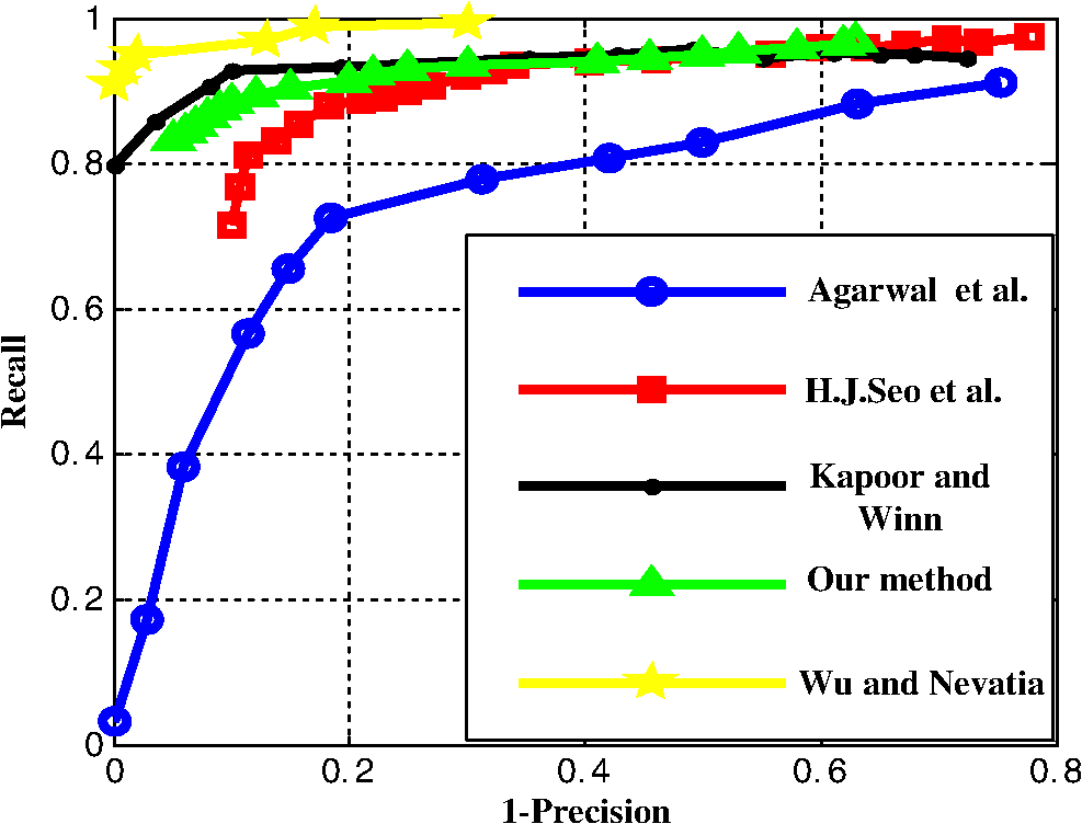

From Fig. 7, it can be observed that our method is better than the methods in Refs. 15 and 39 and the recall is lower than that in Refs. 40 and 41, which need hundreds or thousands of samples. The precision of our method can be improved more if the detected results are combined by querying the object using the training samples one by one. But this is not our main point. Our focus is that detecting the instances of an object by one query using our method is competitive to or better than that of the one-query method executing several times. Compared with the LARK method, because we organize the training samples reasonably, our detection results have more appearance tolerance of the object. Although we just have few samples in hand, the detection result of our method is better than that of the previous works,³⁹ which need hundreds or thousands of samples.

The comparisons of detected equal-error rates (EER)¹⁵ are shown in Tables 1 and 2. One can also find that our proposed method is competitive to or better than those state-of-the-art methods. Here, we compare our method to the state-of-the-art training-based methods^3,39–41 and the one-query method (LARK). The EER on the single- and multiscale test sets are shown in Tables 1 and 2, respectively. From Table 1, it can be found that the EER of our method is higher than that of methods in Refs. 15 and 39, and lower than that of the methods in Refs. 3, 40, and 41. In Table 2, the EER of our method is higher than that of the methods in Refs. 15 and 39 and lower than that of the methods in Refs. 3 and 40. As our strategy is based on few samples, the prior knowledge of the object class is limited. However, the EER of our method also reaches 92.15 and 91.34%, respectively, which are competitive to the methods in Refs. 3, 40, and 41. These methods always need thousands of samples to train classifiers. But our method, whose training processing is much simpler than that of these methods, just needs several samples. Compared to these three methods, our method is also competitive.

Table 1

Detection equal-error rates on the single-scale UIUC car test set.

Ref. 39	77.08%
Ref. 15	88.12%
Ref. 40	94.0%
Ref. 3	98.5%
Ref. 41	97.5%
Our method	92.15%

Table 2

Detection equal-error rates on the multiscale UIUC car test set.

Ref. 39	44.08%
Ref. 15	77.66%
Ref. 40	93.5%
Ref. 3	98.6%
Our method	91.34%

6.2.

Face Detection

In this section, we demonstrate the performance of our method to face detection on Massachusetts Institute of Technology—Carnegie Mellon University (MIT-CMU) face data set⁴² and Caltech face data set.^11,16 The several training samples in our face detection experiments are all chosen from Fundação Educacional Inaciana (FEI) face data set.⁴³ Since we just have few samples in hand, in this section the comparison is only made to the template matching method. As mentioned before, in the template matching methods, the LARK method¹⁵ shows good performance. So we take it as our baseline object detector.

First, we show the detection results of our strategy on MIT-CMU face data set. There are 45 images with 157 frontal faces of various sizes in our test set. The query image and training samples are all adjusted to the size $60\times 60$. The scale of faces in the data set between the largest and smallest is from 0.4 to 2.0. One can see some of the results in Fig. 8. Although the target image is blurry or contains a cartoon human face, our detection method can localize the faces. Especially in Fig. 9, we detect 56 faces correctly among 57 faces and the precision rate is higher than the results in Refs. 15 and 44.

Fig. 8

Detection results on MIT-CMU face data set. Even though the image is blurry, our method also localizes the object. 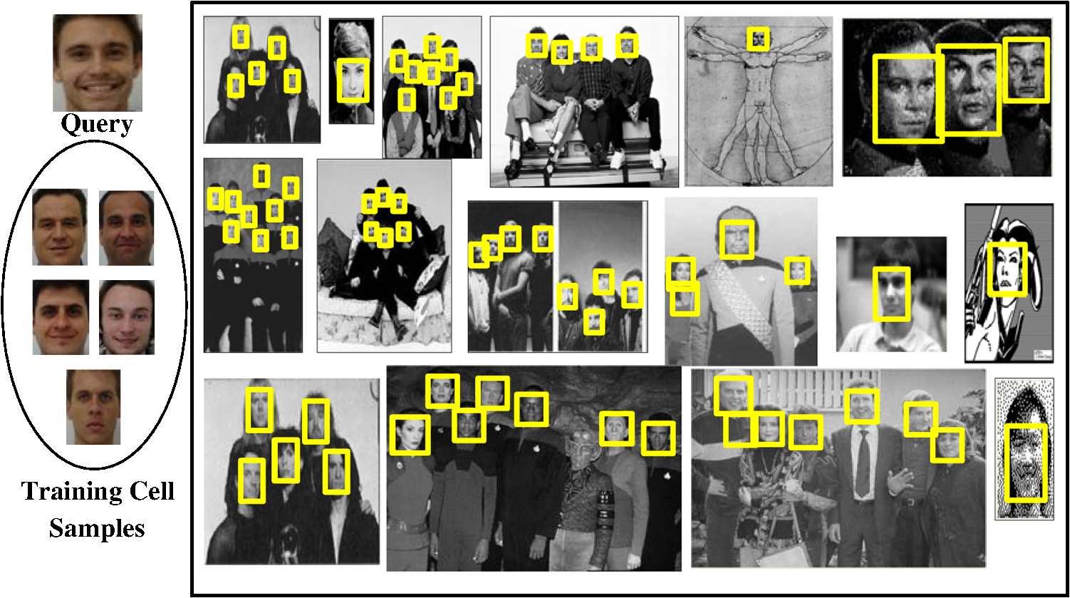${\tau }_L=0.7745$, ${\tau }_S=0.7688$, ${\tau }_{\theta }=0.7911$, and ${\tau }_h=488.6$.

Fig. 9

There are 57 faces in the target image, and our method detects 56 faces with five false alarm. 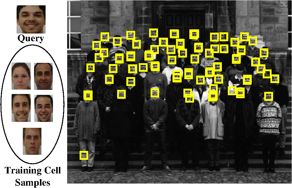${\tau }_L=0.7812$, ${\tau }_S=0.7793$, ${\tau }_{\theta }=0.7704$, and ${\tau }_h=475.1$.

To make a fair comparison, we use the union LARK detection results from several images. For example, if there are six training samples, LARK processes them one by one as the query image. For each target image, we record the true positives of six queries and get the total number of true positives without repeat. In this way, this union multisamples detection result of LARK can be compared with our method fairly. In Fig. 10, we show the comparison between our method and LARK.¹⁵ The curve of our method is the average of five query images with the same training samples. One can find that our method is superior to the LARK.

Fig. 10

Comparison between our proposed method and the union locally adaptive regression kernels (LARK) on MIT-CMU data set. The ROC curve of our proposed method is the average on six query images.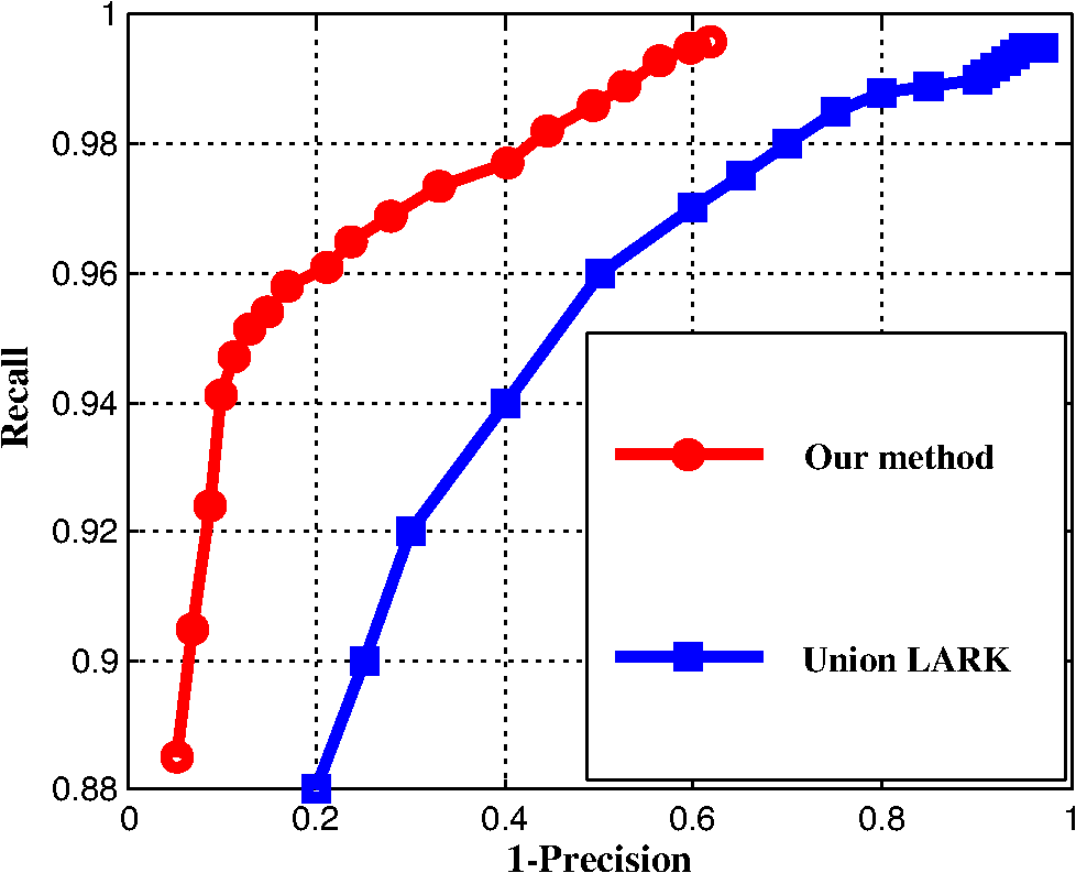

Next, we perform our method on the Caltech^11,16 face data set, which contains 435 frontal faces in file “Faces” with almost the same scale.

The proposed method on three data sets achieves higher accuracy and a lower false alarm rate than that of the union LARK. The organization of the several training samples is more efficient than the one-by-one detection strategy. We draw ROC curves with respect to different query images from the same training samples and to the same query image on different training samples [see Figs. 11(a) and 11(b)] on MIT-CMU face data set. Figure 11 demonstrates that our detection strategy can achieve consistent precisions for both different training samples and different query images. This means our method is robust on different training samples and query images. In fact, we also obtained the same result on other data sets used in this paper. To describe the result clearly, we give the ROC curve on the MIT-CMU face data set.

Fig. 11

ROC curves on MIT-CMU face data set. In (a), we show ROC curves of different query images from the same training samples. In (b), the ROC curves are drawn with the same query image on different training samples.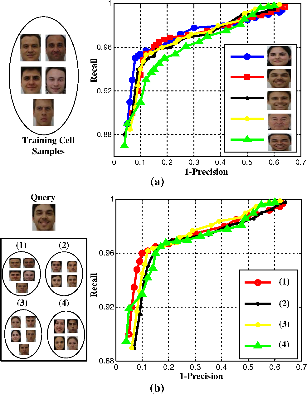

From above, it can be seen that our detection strategy is consistent and robust on different query images and training samples. This is because our detection method has two steps, voting step (VS) and refined hypotheses step (RHS), which measure the object locally and integrally, respectively. Here, we show how these two steps affect our detection results. We compare the detection results of VS + RHS, VS and RHS on the Caltech data set (see Fig. 12). Each curve is drawn and averaged with the same seven query images and three training samples. One can see that the combination of both steps can get a higher precision rate than that of using each step alone, and that the voting strategy along has a higher accuracy than RHS. A similar conclusion can be drawn with other data sets, which are not shown here.

Fig. 12

Comparison of different steps on the Caltech data set. The green curve represents the results that combine both steps. The red curve just uses the voting step. The black curve is using only refined hypotheses step.

6.3.

Generic Object Detection

We have already shown the detection results of our proposed method on the car and face data set. In this section, we use our strategy to some general real-world images containing hearts, flowers, and footballs. To the best of our knowledge, there does not exist a data set for object detection based on a few samples. So we download some real-world images from Google as our data set. One can find these images from our website http://cvlab.uestc.edu.cn/xupei. There are 34 images of red hearts with 49 positive samples and 40 images of sunflowers with 101 positive samples. In all of these data sets, the scale is from 0.2 to 1.8.

The detection examples can be found in Fig. 13. In the real world, the red-heart shape can be found with complex display. So, our detection results contain some false alarms.

Fig. 13

Detection results on general object detection.

6.4.

Time Efficiency Comparison and Feature Comparison

Now we compare the efficiency between our proposed scheme and the detection scheme.¹⁵ For these two methods, there are the same two steps: feature construction and object detection. We compare the time efficiency of these two steps between our strategy and LARK. To formalize the efficiency, $t_{\mathrm{LAS}}^c$ and $t_{\mathrm{LARK}}^c$ are, respectively, defined as the evaluation time of the feature construction. $t_{\mathrm{LAS}}^d$ and $t_{\mathrm{LARK}}^d$ are the evaluation times of the detection step. Here, we define ${\rho }_{\mathrm{LAP}}^c$ and ${\rho }_{\mathrm{LARK}}^c$ to describe the time efficiency of LAS and LARK features, respectively, where

Eq. (24)

$${\rho }_{\mathrm{LAS}}^c=\frac{t_{\mathrm{LAS}}^c}{t_{\mathrm{LAS}}^c+t_{\mathrm{LARK}}^c},$$

Eq. (25)

$${\rho }_{\mathrm{LARK}}^c=\frac{t_{\mathrm{LARK}}^c}{t_{\mathrm{LAS}}^c+t_{\mathrm{LARK}}^c},$$

with a similar definition for ${\rho }_{\mathrm{LAS}}^d$ and ${\rho }_{\mathrm{LARK}}^d$ as

Eq. (26)

$${\rho }_{\mathrm{LAS}}^d=\frac{t_{\mathrm{LAS}}^d}{t_{\mathrm{LAS}}^d+t_{\mathrm{LARK}}^d},$$

Eq. (27)

$${\rho }_{\mathrm{LARK}}^d=\frac{t_{\mathrm{LARK}}^d}{t_{\mathrm{LAS}}^d+t_{\mathrm{LARK}}^d}.$$

One can find the comparison results of LAS and LARK features in Table 3. In the experiment, we evaluate 10 testing times (each testing contains 30 images) to record the evaluation time of the two steps in both our method and the LARK, respectively. In Table 3, we can see that the construction time for LARK feature is more $\sim 30\%$ than that of our LAS feature. This is because the LAS feature just needs to compute the gradients and SVD decomposition to get three parameters. But for LARK feature, after SVD decomposition, the local kernel must be computed and then the principal component analysis (PCA) method is used to reduce the dimension. The superiority of our LAS feature is not just saving memory, but also cutting down the computing steps for each pixel. In Table 3, one can find that ${\rho }_{\mathrm{LAS}}^d$ is also lower $\sim 20\%$% than ${\rho }_{\mathrm{LARK}}^d$ (blue). Our detection step is based on the idea of voting. In Ref. 15, the matrix cosine similarity for each $T_i$ and $Q$ is computed. Then, the salience map is constructed which is very time-consuming. In our method, the time of the training step can be ignored. In the experiments, we find that the consuming time of the training step is $<7\%$ of the whole running time for detecting objects in a target image.

Table 3

Comparison of efficiency between LAS and LARK.

Testing times	1	2	3	4	5	6	7	8	9	10
${\rho }_{\mathrm{LARK}}^c$	71%	72%	71.5%	73%	74%	73%	72%	71%	71%	70%
${\rho }_{\mathrm{LAS}}^c$	29%	28%	28.5%	27%	26%	27%	28%	29%	29%	30%
${\rho }_{\mathrm{LARK}}^d$	58%	59%	57%	60%	61%	59%	61%	62%	59%	60%
${\rho }_{\mathrm{LAS}}^d$	42%	41%	43%	40%	39%	41%	39%	38%	41%	40%

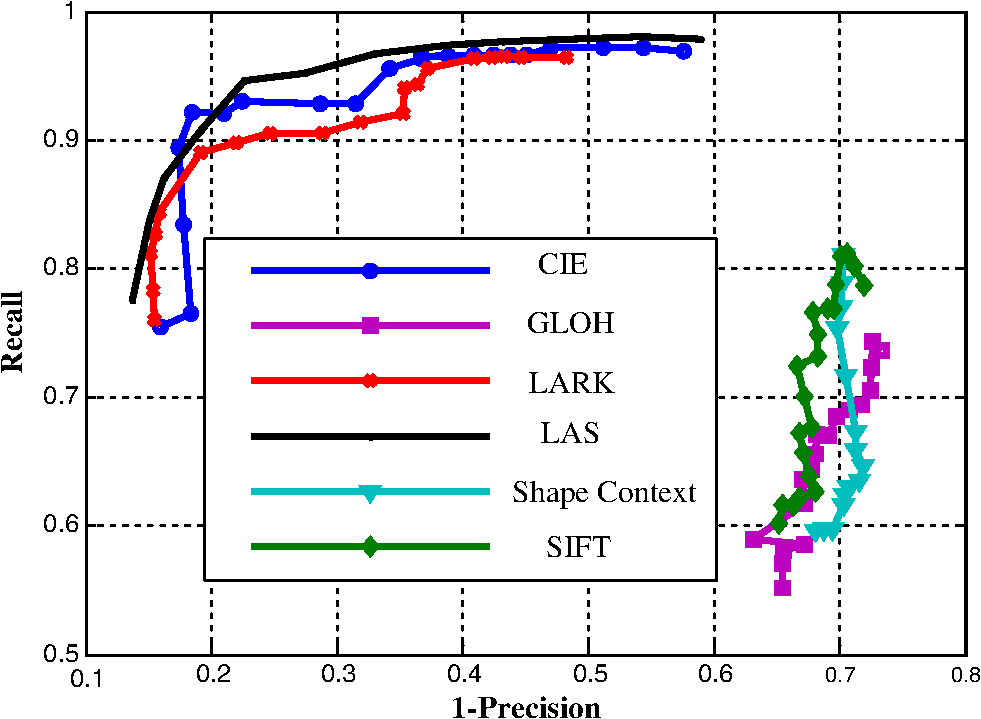
We further compare the performance with some art local features on Shechtman and Irani’s test set.¹² We use our LAS feature to compare with gradient location-orientation-histogram (GLOH),⁴⁵ LARK,¹⁵ Shape Context,⁴⁶ SIFT,¹⁷ and Commission Internationale de L’Eclairage (CIE).¹² The ROC curves can be seen in Fig. 14. Compared to previous works, our LAS feature is much better than SIFT, Shape Context, and GLOH in the case of a few samples. Comparing to CIE and LARK, our LAS feature is comparable or even better.

Fig. 14

Comparison of different kinds of features on Shechtman and Irani’s test set.¹² Gradient location-orientation-histogram,⁴⁵ LARK,¹⁵ Shape Context,⁴⁶ SIFT¹⁷ and CIE.¹²

7.

Conclusion and Future Work

In this paper, we proposed a generic objects detection method based on few samples. We used the local principal gradient orientation variation information, namely LAS, as our feature. The voting spaces are trained based on a few samples. Our detection method contains two steps. The first step is adopting a combination densely voting method in trained voting spaces to detect similar patches in target image. Through the construction of a voting space, the advantage of our approach is resilient to local deformation of appearance. Then, a refined hypotheses step is used to locate object accurately.

Compared with the state-of-the-art methods, our experiments confirm the effectiveness and efficiency of our method. Our LAS feature has more efficiency and memory saving than that of LARK. Besides, the strategy we proposed in this paper gives a method of object detection when the samples are limited. Previous template matching method is to detect objects using samples one by one, while our method is to organize several samples to detect objects once. In the future, we will extend our work to the problem of multiple-object detection and improve the efficiency further.