|
|
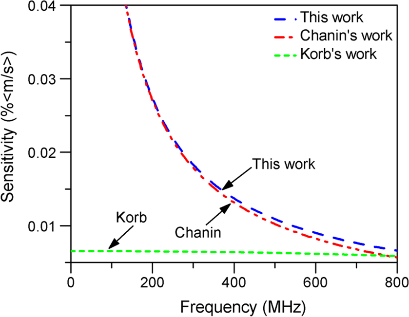
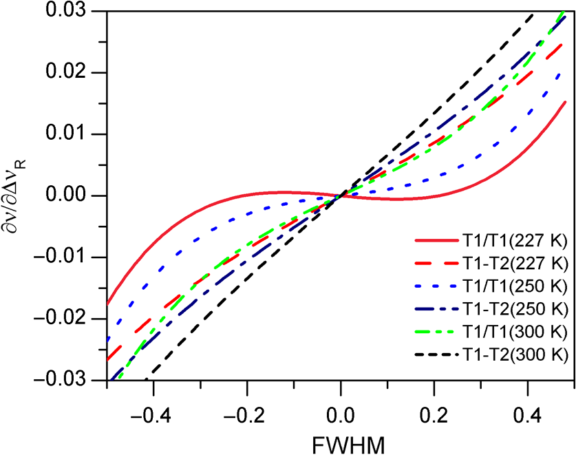
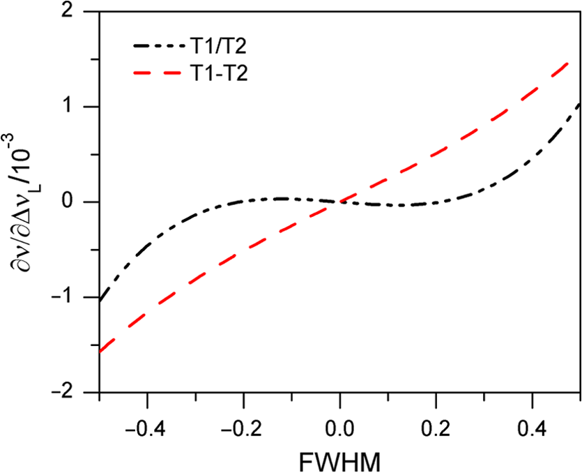
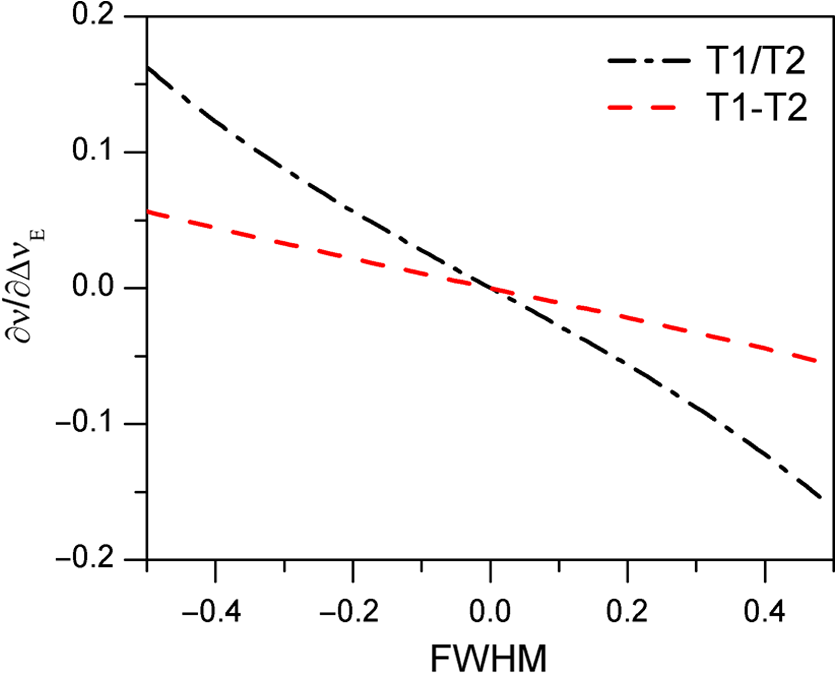
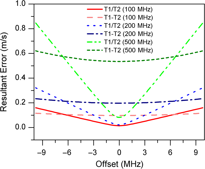
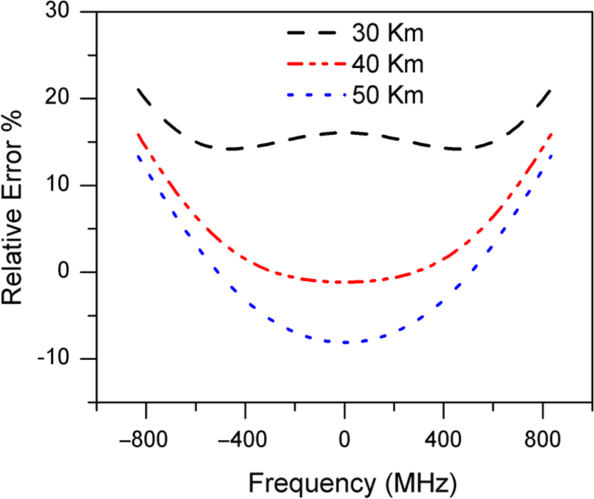
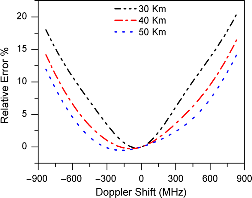
1.IntroductionWind observation throughout the troposphere and low stratosphere is one of the most important and challenging tasks for improving numerical weather prediction, hurricane tracking, pollution tracing, and understanding of mesoscale dynamic process, transport, and exchange in the atmosphere. Many instruments and techniques are widely used to obtain wind data, for example, radiosondes, balloons, sounding rockets, ground-based wind profilers. But they still cannot fulfill the unmet information of the global wind fields with needed accuracy and resolution. Doppler wind lidar is now regarded as the potential way to fill the gaps limited by the method mentioned above.1,2 Currently, there are two primary categories of wind-sensing lidar: coherent and direct detection lidar. Coherent lidar measures the Doppler shift by beating the backscattered signal with light from a continuous-wave local oscillator laser, which often resolves the narrowband aerosol and cloud return and is commonly used for relatively small velocity detection.3 The theory of direct-detection Doppler wind lidar was first described and realized by Benedetti-Michelangeli et al.4 Various kinds of instruments, such as Fabry–Perot interferometer (FPI),5–10 iodine absorption filter,11,12 Fizeau interferometer,13 and Mach–Zehnder interferometer,14 have been chosen to discriminate the Doppler shift from the spectrally broadband Rayleigh–Brillouin return of molecules and spectrally narrowband Mie backscatter return of aerosol or cloud particles. The Doppler shift determination for direct detection has two typical implementations: edge technique and fringe-imaging technique. The edge technique uses one or more narrowband filters to transform the Doppler shift into an irradiance variation,5–8,15 whereas the fringe-imaging technique retrieves the Doppler shift from the radial angular distribution or spatial movement of the interference patterns of an interferometer.16,17 The double-edge technique as a powerful variation of the single-edge technique used for retrieving the instantaneous wind information has been demonstrated by Korb et al.7,8 It inherits the advantage of edge technique and extends its capabilities but has higher measurement precision. In the Atmospheric Dynamic Mission Aeolus (ADM-Aeolus) payload Atmospheric Laser Doppler Instrument (ALADIN), the double-edge technique will be used to analyze the molecular Rayleigh return with two FPIs as discriminator.18,19 For wind measurement in the upper troposphere and stratosphere, Rayleigh Doppler lidar is the only remote sensing instrument because in such altitude, Mie backscattering signal is very weak in most situations except after intense volcano eruptions. Two FPIs with opposite slopes symmetrically located at the wings of the atmospheric Rayleigh spectrum are used to discriminate the Doppler shift. As performed in the Observatory of Haute Provence in France, the Rayleigh lidar has demonstrated the possibility of continuous monitoring of the variability of the middle atmosphere.20,21 Chanin et al.5 and Garnier and Chanin6 gave an instrument description and the method for wind retrieval in 1989. Different from the method of Chanin, Flesia and Korb described the wind determination algorithm for double-edge molecular technique in detail in 1999.8 The measurement precision related to the instrument performance was discussed by McGill and Spinhirne through modeling the Doppler wind lidar techniques and making improvement on general instrument design.17 In order to make the model more intuitive and conveniently implemented, McKay developed an another analytical model considering aperture finesse effects of FPI and background noise.15 However, besides the system performance, the retrieval method itself as another primary factor impact on the measurement precision is rarely discussed. In this article, we pay attention to the measurement precision of various retrieval methods used for wind detection and analyze their stabilities in the case that there exist spectrum width deviations in laser pulse, Rayleigh backscatter, and FPI transmission curve. The result of simulation shows that the retrieval method proposed in this article is especially suited for altitude with large wind speed. Section 2 gives a review of the existing retrieval theory. In Sec. 3, we propose a new frequency response function and then compare it to the existing methods especially in the situation of the splitting ratio of the double-edge channels being not exactly . Section 4 presents the algorithm stability discussion for spectrum width uncertainties of laser pulse, Rayleigh backscatter, and FPI transmission curves. We give a comprehensive analysis in Sec. 5 and the Conclusion is presented in Sec. 6. 2.Review of Retrieval Methods in ExistenceWe first give a review of double-edge lidar technique for wind measurement with the molecular signal backscattered from the atmosphere, which has been described by several groups.5–8,20–25The molecular signal with Doppler shifts is spectrally broadened due to the random thermal motion of the molecules and Brillouin scattering.26–29 As shown in Fig. 1, we use two FPIs, labeled Edge1 and Edge2, located at the wings of the atmospheric Rayleigh spectrum to discriminate the Doppler shift from the Rayleigh backscatter. Due to the steep slope of the edge filter, a small frequency shift can cause relatively large changes in measured signal. Wind detection is implemented by measuring the transmission changes of the backscattering on the double-edge channels. Fig. 1Spectrum of the atmospheric backscattered Rayleigh signal along with two Fabry–Perot interferometer (FPI) transmission functions. The dotted green line and dashed dotted green line are Rayleigh spectrum without Doppler shift and with Doppler shift of , respectively. The cavity spacing of FPI is 12.5 cm, with free spectral range (FSR) of 12 GHz. The full width at half maximum (FWHM) of the FPI transmission curve is 1.7 GHz.  A small portion of the outgoing laser beam is split as a reference signal to monitor its frequency by measuring its location on the edge of the filter. The signal backscattered from the atmosphere is split by two beamsplitters into the double-edge channels and an energy monitor channel for normalization, as shown in Fig. 2. The signals incident to the double-edge channels transmit through the twin FPI and then are detected by two detectors. The operating wavelength is chosen to be in the ultraviolet at 355 nm to take advantage of the dependence of the molecular backscatter. Fig. 2Schematic of multichannels signal processing. (IF, interference filter; BS, beamsplitter; Det, detector). 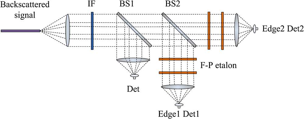 The radial wind, bulk motion of atmosphere in line of sight, causes an overall spectral Doppler shift , which can be determined from a differential measurement of the frequency of the laser return from the atmosphere. This makes the measurement insensitive to the laser frequency jitter and shift.30 In order to retrieve the Doppler shift from the backscattered signals, Chanin et al.5 defined a Doppler frequency response function R as follows: where NA and NB are the number of photons backscattered from a layer of vertical thickness centered at some height and then transmitted through two edge filters and finally detected by two photomultipliers. C is a corrective factor determined experimentally.5 Different from the algorithm of Chanin et al., Korb and Gentry7 gave another definition of which can be written aswhere and are the signal intensity measured by the two edge filters, respectively.7,8 The response function is sensitive to the wind’s speed and provides a unique measurement of them. Although the two retrieval methods have been used for about two decades, there are still some problems under solving, e.g., whether there is alternative retrieval proposals possible to improve the measurement precision considering shot-noise-limited and whether the measurement is sensitive to the deviations of the laser spectrum width, Rayleigh spectrum width, and the full width at half maximum (FWHM) of the interferometer transmission curve. This article offers a reasonable solution to the problems mentioned above.3.Sensitivity and Error DiscussionsIn this work, we mainly discuss the measurement error of various retrieval methods for Rayleigh spectrum in practice case. The parameters of the FPI we chose are based on the principle that Rayleigh and aerosol spectrum have the same velocity sensitivity, which is similar to the description of Flesia and Korb.8 As a result, the measurement is desensitized to the effects of aerosol scattering. In order to simplify the process of the discussion, we first rewrite the frequency response function . As we know, the number of photons transmitted through the edge filters is proportional to their transmissions on them. Therefore, the proposed by Chanin et al.5 can be rewritten as Similarly, the for the analysis method of Flesia and Korb8 is given by and are the transmissions on the FPI. Mckay pointed out that the methods displayed in Eqs. (3) and (4) actually had the same measurement error.31 They are the special cases for the methods of transmission ratio [the in Eq. (3) substantially is a function of ] but have different sensitivities. For double-edge technique, except for transmission ratio, another most intuitional idea we can imagine is the transmission subtraction, which defines the frequency response function as The transmission subtraction is the new proposed method for Rayleigh Doppler lidar wind determination and its superiority under some circumstances would be shown in the following discussion. 3.1.SensitivityFor Rayleigh Doppler wind lidar, one of the key parameters that must be considered is the measurement sensitivity, which converts the fractional error in the measurement into an error in meters per second. The sensitivity of the double-edge measurement is the fractional change of the frequency response function for a unit wind velocity which can be written as Korb gave the whole calculation process for his analysis method and the result is given by where(, 2) are the sensitivities of the molecular measurement for a single edge. Similarly, we give the measurement sensitivity of Chanin et al.’s method as follows: Equation (6) gives us the definition of the double-edge measurement sensitivity. For the method we proposed in this article , whose sensitivity can be deduced as follows: Figure 3 shows the measurement sensitivities of the three methods as a function of the frequency separated from the crossover point of the twin FPI transmission curves. In view of the symmetry, only the sensitivity versus positive Doppler shift is displayed. As shown, the sensitivity of Flesia and Korb’s method almost keeps constant as the frequency increases, whereas the other two decrease dramatically. The measurement sensitivities of the new method and Chanin et al.’s method are higher than Flesia and Korb’s and their line types tend to be highly similar to each other especially for small Doppler shift. For greater Doppler shift, a typical value of 700 MHz, which is equal to a wind velocity of about , and their sensitivities are in close proximity to each other. Actually, such high wind speed is extremely rare even in the stratosphere up to 60-km altitude. Therefore, the new proposed method together with Chanin et al.’s method is thought to have a higher measurement sensitivity that indicates for a given error, a lower signal-to-noise ratio (SNR), and thus a shorter integration time is required. This is of prime importance for a molecular measurement while the sensitivity is lower than for a corresponding aerosol-based measurement by a factor of .7,8 3.2.Error AnalysisHere, we continue to use the error estimate method described in Korb et al.’s and Flesia and Korb’s work,7,8 where the error in the line of sight wind is given by SNR and are the SNR and the sensitivity for the double-edge measurement, respectively. The sensitivities of the three methods have been discussed in the last subsection. Another pivotal parameter for error estimate is the SNR of measurement which is given on the assumption that the noise measured in different channels can be considered to be uncorrelated, as used in Korb et al.’s article for the description of edge technique.30 First, the measurement SNR can be written as where is the variance of , it is given by where and are the signals of double-edge channels and is the signal of energy monitor channel, respectively. Similarly,Then, from Eq. (11), the measurement errors are It is easy to find that the results of Korb et al.’s and Chanin et al.’s method are the same. The following statement demonstrates it not to be an accident and all the frequency response functions have the same estimated error only if they can be written as a function of transmission ratio, i.e., . Under the premise as a function of , then Eq. (13) can be rewritten as Note that the last term equals 0 and then So, the SNR can be written as We calculate the sensitivity as follows: Then, from Eqs. (20) and (21), the measurement error is The demonstration indicates that all the efforts try to make the measurement better through transmission ratio is unavailing. The error due to the SNR is dominated typically by the SNR of the double-edge channels for the method of transmission ratio, whereas the energy monitor channels should also be taken into consideration for transmission subtraction. However, for a certain signal backscattered from the atmosphere, the SNR of the three channels is partly determined by the splitting ratio. From the perspective of mathematics, it is easy to find from Eq. (22) that the minimum error occurs only if the splitting ratio of the double-edge channels is exactly , which is very difficult to realize in the engineering practicality. Figure 4 shows the measurement errors of two different ways as a function of the splitting ratio of the double-edge channels at a Doppler shift of 200 MHz. As shown, the two methods have their own superiority as the splitting ratio varies. However, the splitting ratio is a fixed value immediately after the calibration. In other words, if the splitting ratio is at the right side of the crossing point, value of about 1.1, the new method would have a better performance. We can facilitate our grasp of the result in this way. The backscattered signal with a Doppler shift makes the transmission increase on one edge filter and decrease on another one. The minimum error for corresponding wind velocity occurs when the edge channel with lower transmission occupies a higher percentage of the general signals of the double-edge channels to compensate for the differentiated SNR. It is necessary to point out that the signal intensity of the energy monitor channel we used to analyze the measurement error is about 10% of the whole signal. Thus, the transmissions of the double-edge channels at the cross point are about 20%, which leads to a relatively small error due to approximately equal SNRs of the three independent channels according to Eq. (17). Figure 5 gives the relative error of the two retrieval methods at various altitudes for typical splitting ratios 1.1 and 1.2 as a function of Doppler shift. The relative error is defined as , where the and are errors of transmission ratio and transmission subtraction, respectively. It shows that for small Doppler shift, the new proposed method has a relatively smaller error and the higher the splitting ratio, the more obvious the difference between the two methods. Fig. 5For typical splitting ratio, the relative error of two retrieval methods as a function of frequency.  Although the relative error shown in Fig. 5 is very small () even at the peak of the curve, it is still significant because the measurement precision is not totally determined by the sensitivity and SNR. As described earlier, the frequency response function as a function of transmissions on the double-edge channels is sensitive to the transmission curves. However, the transmission function for Rayleigh backscatter is a convolution of the FPI transmission function, laser spectrum, and the Rayleigh spectrum. So, the stabilities of the retrieval methods to three spectrum widths are another primary error source that we must consider, which is discussed in the next section. 4.Algorithm StabilityAs mentioned in the last section, the spectrum widths of the edge function, laser spectrum, and the Rayleigh spectrum are potential parameters that may cause measurement errors. Therefore, it is necessary to do research on the differential relations of frequency response function which reveal how the Doppler frequency relies on the spectrum widths. Similarly, we define the measurement sensitivities for FWHM of the FPI, width of the laser spectrum, and Rayleigh spectrum as follows: The ultimate object of all the endeavors is to obtain the relationship between the Doppler shift uncertainty and ones of various spectrum widths. However, the Doppler shift, as an inverse function of , is indirectly related to spectrum widths mentioned above. Theoretically, the partial derivative of the Doppler shift to a certain spectrum width is given by where stands for one of the spectrum widths and thus is its sensitivity. Equation (24) provides the fundamental formula for the discussion of the retrieval methods’ stability. We substitute the frequency response function for Eqs. (3) and (4), respectively. The result shows that the method of Chanin et al. and Korb et al. has the same stability even if there is a factor of difference in the sensitivity as mentioned in Sec. 2. That is because for an arbitrary spectrum width, there is still the same factor in difference. We give the derivative relation for transmission ratio as follows:However, the manner of transmission subtraction shows distinct differences compared to transmission ratio. Neglecting the mathematic operating, the derivative relation for signal subtraction is given by Figure 6 shows the partial derivative of Doppler shift with respect to the Rayleigh spectrum width as a function of the frequency in unit of FWHM of the FPI. According to U.S. standard atmosphere 1976, for different temperatures relevant to different altitudes of 30, 40, and 50 km, the proposed method is more acute to the deviation of the Rayleigh spectrum with an order of , as shown in Fig. 6. Another two partial derivations are shown in Figs. 7 and 8, respectively. The line shape displayed in Fig. 7 is very analogous to that in Fig. 6 because the Rayleigh spectrum contributes to Doppler shift in the same manner with the laser spectrum. However, the influence of laser spectrum width on Doppler shift is much smaller compared to the Rayleigh spectrum width. Besides, it is easy to find that Korb et al.’s method is more sensitive to the FWHM of FPI. The resultant error caused by various spectrum widths can be calculated by where , , and are the spectrum width uncertainties of the Rayleigh, laser, and FPI, respectively.It seems that the method of transmission subtraction may cause higher measurement errors due to more likely be affected by uncertainties of the laser and Rayleigh spectrum widths, the following analysis can help us dispel the concern about this. The error caused by the laser spectrum width can be neglected for two reasons: one is the well stable performance of the laser and thus little frequency jitter and drift; another is that the derivative of the Doppler shift with respect to the laser spectrum width is about 1 or 2 orders of magnitude smaller than the other two widths. The Rayleigh spectrum width varies as the square root of the atmospheric temperature. The error occurs when the value used for the atmospheric temperature does not match the actual atmospheric temperature. Supposing a 5-K error in our knowledge of the atmospheric temperature profile, this causes a 38-MHz deviation of the Rayleigh width at 220 K. In view that the derivative coefficient of Rayleigh width is only 1 order of magnitude smaller than that of the FPI FWHM, although the Rayleigh width related error cannot be neglected, it is only the secondary error source. Many factors may lead to changes of the FPI transmission curves, such as the voltage added to the piezoelectric actuators, ambient temperature, and the stability of the illumination during the wind detection. From Fig. 8, we can find that the algorithm of transmission subtraction is relatively insensitive to the changes of FPI FWHM. Although the standard deviation of the FWHM can decline to by repeating the scanning experiment, the error is still the primary one because the partial derivative is about 1 or 2 orders of magnitude larger than the two spectrum widths. We assume a 2-MHz error in laser width and 40 MHz in Rayleigh width which is near the limit to our knowledge of temperature profile. For three typical Doppler shifts, 100, 200, and 500 MHz, whose relevant wind velocities are 18, 35, and , respectively, Fig. 9 gives the resultant errors of the two methods as a function of the FPI FWHM deviation. As shown, the new proposed method generally varies gently to the drift of the FPI FWHM. We can see that the cross point of the two curves at any Doppler shift is about 6.5 MHz, which indicates when the deviation between the FPI FWHM we used to determine the wind velocity and its real value is larger than this value, the proposed method would have a better performance. In order to reveal the difference between the two methods more intuitively, we choose an FPI FWHM offset of 8 MHz and calculate the relative error, as shown in Fig. 10. As a result of Eq. (31), it shows us the relative error of the two retrieval methods at various altitudes. It should be noticed that the curve of 30-km altitude is much different than the other two. Actually, at such height level, not only the FWHM offset of FPI but also the deviation of the Rayleigh spectrum width dominates the relative error. From Fig. 6, we can find that the difference value between the two retrieval methods at 30-km altitude (227 K, U.S. Standard Atmosphere 1976) is of the same order of magnitude compared to that of the FPI FWHM in Fig. 8. Meanwhile, the difference value reaches its maximum at about FWHM of the FPI (about 550 MHz) in Fig. 6, where the relative error in Fig. 10 reaches its minimum. This well explains the difference between 30 km and other altitudes. 5.AnalysisWe have discussed the measurement error in situation of shot-noise-limited in Sec. 3 and the errors caused by the instability of various spectrum widths in Sec. 4. Actually, these two factors behave simultaneously throughout the wind detection and we must synthetically think them over. The frequency response function can be written as The Doppler shift is derived from Eq. (32) and it can be expressed as Then the error is given as follows: Actually, the first term is the measurement error because whereas the sum of last three terms is the error caused by algorithm instability as described in last section. Equation (33) gives a comprehensive reflection of the errors and we can infer from it that the algorithm stability cannot be ignored when the error caused by system SNR is equivalent to the one introduced by deviations of various spectrum widths. Although the real SNR cannot be obtained without experiment due to various temporal and spatial resolutions, we select a value large enough to meet the conditions mentioned above, which typically guarantee the measurement error of about 1 to at 30 km altitude. A relative error for the two retrieval methods in condition of splitting ratio of 1.2 and FPI FWHM offset of 8 MHz is given in Fig. 11.As shown, for the altitude of 30 km, the proposed method reduces the measurement error from to as the Doppler shift varies. Even if it generally tends to be smaller for other two altitudes, it is still meaningful. On the one hand, more precise temperature estimate can make the advantages of transmission subtraction more obvious because it is more sensitive to the change of temperature compared to transmission ratio. On the other hand, the FPI FWHM deviation of 8 MHz is a very critical requirement for the experiment. In addition, all the discussion and comparison we made in this article shows that there is no substantive difference between the method of Korb et al. and Chanin et al. except for the sensitivity. 6.ConclusionsA new retrieval method is described by introducing a new frequency response function. Compared to other frequency response functions proposed by Korb et al. and Chanin et al., it has a higher sensitivity. In the actual situation of splitting ratio to be not exactly , it shows its superiority especially for small Doppler shift and thus small wind velocity. Algorithm stability, i.e., errors caused by deviations of various spectrum widths, is first discussed and it can reach a few tenths of 1 meter per second. Well-stable laser performance and relative accurate knowledge of temperature profile guarantee the new proposed method has less sensitivity to deviations of spectrum widths. Comparison between the new method and the existing algorithm under overall consideration is performed. The result shows that the new proposed method decreases the resultant error from to as the Doppler shift varies with the splitting ratio of 1.2 and the FPI FWHM deviation of 8 MHz. It is necessary to point out that the new method is extremely suited for circumstances of low atmosphere temperature, uncoordinated splitting ratio, and nonignorable error caused by algorithm instability. This article also demonstrates that there is no substantive difference between the methods of Korb et al. and Chanin et al. except for the measurement sensitivity. This indicates that we cannot figure on the manner of transmission ratio to improve the measurement accuracy. AcknowledgmentsThis work was funded by the CAS Special Grant for Postgraduate Research, Innovation and Practice and the National Natural Science Foundation of China (NSFC) project Nos. 41174130, 41304123, and 41174131. ReferencesA. Stoffelenet al.,
“The atmospheric dynamics mission for global wind field measurement,”
Bull. Am. Meteorol. Soc., 86
(1), 73
–87
(2005). http://dx.doi.org/10.1175/BAMS-86-1-73 BAMIAT 0003-0007 Google Scholar
P. Hayset al.,
“Space-based Doppler winds lidar: a vital national need,”
in Response to national research council (NRC) decadal study request for information (RFI),
(2005). Google Scholar
R. M. HuffakerR. M. Hardesty,
“Remote sensing of atmospheric wind velocities using solid-state and coherent laser systems,”
Proc. IEEE, 84
(2), 181
–204
(1996). http://dx.doi.org/10.1109/5.482228 IEEPAD 0018-9219 Google Scholar
G. Benedetti-MichelangeliF. CongedutiG. Fiocco,
“Measurement of aerosol motion and wind velocity in the lower troposphere by Doppler optical radar,”
J. Atmos. Sci., 29
(7), 906
–910
(1972). http://dx.doi.org/10.1175/1520-0469(1972)029<0906:MOAMAW>2.0.CO;2 JAHSAK 0022-4928 Google Scholar
M. L. Chaninet al.,
“A Doppler lidar for measuring winds in the middle atmosphere,”
Geophys. Res. Lett., 16
(11), 1273
–1276
(1989). http://dx.doi.org/10.1029/GL016i011p01273 GPRLAJ 0094-8276 Google Scholar
A. GarnierM. L. Chanin,
“Description of a Doppler Rayleigh lidar for measuring winds in the middle atmosphere,”
Appl. Phys. B, 55
(1), 35
–40
(1992). http://dx.doi.org/10.1007/BF00348610 APBOEM 0946-2171 Google Scholar
C. L. Korbet al.,
“Theory of the double-edge technique for Doppler lidar wind measurement,”
Appl. Opt., 37
(15), 3097
–3104
(1998). http://dx.doi.org/10.1364/AO.37.003097 APOPAI 0003-6935 Google Scholar
C. FlesiaC. L. Korb,
“Theory of the double-edge molecular technique for Doppler lidar wind measurement,”
Appl. Opt., 38
(3), 432
–440
(1999). http://dx.doi.org/10.1364/AO.38.000432 APOPAI 0003-6935 Google Scholar
J. WuJ. WangP. B. Hays,
“Performance of a circle-to-line optical system for a Fabry–Perot interferometer: a laboratory study,”
Appl. Opt., 33
(34), 7823
–7828
(1994). http://dx.doi.org/10.1364/AO.33.007823 APOPAI 0003-6935 Google Scholar
T. D. IrgangP. B. HaysW. R. Skinner,
“Two-channel direct-detection Doppler lidar employing a charge-coupled device as a detector,”
Appl. Opt., 41
(6), 1145
–1155
(2002). http://dx.doi.org/10.1364/AO.41.001145 APOPAI 0003-6935 Google Scholar
C. Nagasawaet al.,
“Incoherent Doppler lidar using wavelengths for wind measurement,”
Proc. SPIE, 4153 338
–349
(2001). http://dx.doi.org/10.1117/12.417066 PSISDG 0277-786X Google Scholar
Z.-S. Liuet al.,
“Low-altitude atmospheric wind measurement from the combined Mie and Rayleigh backscattering by Doppler lidar with an iodine filter,”
Appl. Opt., 41
(33), 7079
–7086
(2002). http://dx.doi.org/10.1364/AO.41.007079 APOPAI 0003-6935 Google Scholar
J. A. McKay,
“Assessment of a multibeam Fizeau wedge interferometer for Doppler wind lidar,”
Appl. Opt., 41
(9), 1760
–1767
(2002). http://dx.doi.org/10.1364/AO.41.001760 APOPAI 0003-6935 Google Scholar
D. Bruneauet al.,
“Wind velocity lidar measurements by use of a Mach–Zehnder interferometer, comparison with a Fabry–Perot interferometer,”
Appl. Opt., 43
(1), 173
–182
(2004). http://dx.doi.org/10.1364/AO.43.000173 APOPAI 0003-6935 Google Scholar
J. A. McKay,
“Modeling of direct-detection Doppler wind lidar. I. The edge technique,”
Appl. Opt., 37
(27), 6480
–6486
(1998). http://dx.doi.org/10.1364/AO.37.006480 APOPAI 0003-6935 Google Scholar
J. A. McKay,
“Modeling of direct-detection Doppler wind lidar. II. The fringe imaging technique,”
Appl. Opt., 37
(27), 6487
–6493
(1998). http://dx.doi.org/10.1364/AO.37.006487 APOPAI 0003-6935 Google Scholar
M. J. McGillJ. D. Spinhirne,
“Comparison of two direct-detection Doppler lidar techniques,”
Opt. Eng., 37
(10), 2675
–2686
(1998). http://dx.doi.org/10.1117/1.601804 OPEGAR 0091-3286 Google Scholar
O. Reitebuchet al.,
“The airborne demonstrator for the direct-detection Doppler wind lidar ALADIN on ADM-Aeolus. Part I: Instrument design and comparison to satellite instrument,”
J. Atmos. Ocean. Technol., 26
(12), 2501
–2515
(2009). http://dx.doi.org/10.1175/2009JTECHA1309.1 JAOTES 0739-0572 Google Scholar
U. Paffrathet al.,
“The airborne demonstrator for the direct-detection Doppler wind lidar ALADIN on ADM-Aeolus. Part II: Simulations and Rayleigh Receiver Radiometric performance,”
J. Atmos. Ocean. Technol., 26
(12), 2516
–2530
(2009). http://dx.doi.org/10.1175/2009JTECHA1314.1 JAOTES 0739-0572 Google Scholar
C. Souprayenet al.,
“Rayleigh-Mie Doppler wind lidar for atmospheric measurements. I. Instrumental setup, validation, and first climatological results,”
Appl. Opt., 38
(12), 2410
–2421
(1999). http://dx.doi.org/10.1364/AO.38.002410 APOPAI 0003-6935 Google Scholar
C. SouprayenA. GarnierA. Hertzog,
“Rayleigh-Mie Doppler wind lidar for atmospheric measurements. II. Mie scattering effect, theory, and calibration,”
Appl. Opt., 38
(12), 2422
–2431
(1999). http://dx.doi.org/10.1364/AO.38.002422 APOPAI 0003-6935 Google Scholar
C. FlesiaC. L. KorbC. Hirt,
“Double-edge molecular measurement of lidar wind profiles at 355 nm,”
Opt. Lett., 25
(19), 1466
–1468
(2000). http://dx.doi.org/10.1364/OL.25.001466 OPLEDP 0146-9592 Google Scholar
B. M. GentryH. ChenS. X. Li,
“Wind measurements with 355 nm molecular Doppler lidar,”
Opt. Lett., 25
(17), 1231
–1233
(2000). http://dx.doi.org/10.1364/OL.25.001231 OPLEDP 0146-9592 Google Scholar
H. Xiaet al.,
“Febry-Perot interferometer based Mie Doppler lidar for low tropospheric wind observation,”
Appl. Opt., 46
(29), 7120
–7131
(2007). http://dx.doi.org/10.1364/AO.46.007120 APOPAI 0003-6935 Google Scholar
H. Xia,
“Mid-altitude wind measurements with mobile Rayleigh Doppler lidar incorporating system-level optical frequency control method,”
Opt. Express, 20
(14), 15286
–15300
(2012). http://dx.doi.org/10.1364/OE.20.015286 Google Scholar
A. SugawaraS. Yip,
“Kinetic model analysis of light scattering by molecular gases,”
Phys. Fluids, 10
(9), 1911
–1921
(1967). http://dx.doi.org/10.1063/1.1762387 PHFLE6 1070-6631 Google Scholar
G. TentiC. D. BoleyR. D. Desai,
“On the kinetic model description of Rayleigh–Brillouin scattering from molecular gases,”
Can. J. Phys., 52
(4), 285
–290
(1974). CJPHAD 0008-4204 Google Scholar
G. TentiR. D. Desai,
“Kinetic theory of molecular gases Iymodels of the linear Waldmann–Snider collision operator,”
Can. J. Phys., 53
(13), 1266
–1278
(1975). http://dx.doi.org/10.1139/p75-162 CJPHAD 0008-4204 Google Scholar
C. D. BoleyR. D. DesaiG. Tenti,
“Kinetic models and Brillouin scattering in a molecular gas,”
Can. J. Phys., 50
(18), 2158
–2173
(1972). http://dx.doi.org/10.1139/p72-286 CJPHAD 0008-4204 Google Scholar
C. L. KorbB. GentryC. Weng,
“The edge technique: theory and application to the lidar measurement of atmospheric winds,”
Appl. Opt., 31
(21), 4202
–4213
(1992). http://dx.doi.org/10.1364/AO.31.004202 APOPAI 0003-6935 Google Scholar
J. A. Mckay,
“Comment on “Theory of the double-edge molecular technique for Doppler lidar wind measurement,”
Appl. Opt., 39
(6), 993
–996
(2000). http://dx.doi.org/10.1364/AO.39.000993 APOPAI 0003-6935 Google Scholar
BiographyYuli Han received his BS degree in applied physics from University of Science and Technology of China in 2007. He is pursuing his PhD degree at the University of Science and Technology of China. His current research interests include all-optical signal processing and laser remote sensing. Xiankang Dou is a professor of University of Science and Technology of China. His current research field include stratosphere, mesosphere, and lower thermosphere (SMLT) dynamics and waves, laser remote sensing technology and lidar atmospheric sensing. Dongsong Sun is a professor of University of Science and Technology of China. His current research interests include lidar technology, lidar remote sensing, and Doppler wind lidar technology. Haiyun Xia received the BS degree in physics and MS degree in optics from Soochow University, China, in 2003, and 2006, respectively, and the PhD degree in optoelectronics as a joint training student from the Beijing University of Aeronautics and Astronautics and the University of Ottawa, in 2011. Upon graduation, he joined University of Science and Technology of China as an associate professor. His current research interests include all-optical signal processing, ultra-short laser pulse characterization and applications to high-speed optical sensing, fiber-optic sensors and laser remote sensing. Zhifeng Shu received the BS degree in physics from China university of Petroleum in 2007. The M.S. degree and PhD degree in optics from Anhui Institute of Optics and Fine Mechanics, Chinese Academy of Sciences in 2009 and 2012, respectively. Upon graduation, he joined University of Science and Technology of China as a postdoctorate. His current research interests include all-optical signal processing, photo-detection and laser remote sensing. |