
|
|
1.IntroductionThere are very few options available to probe the interior of the ocean remotely. Both active and passive acoustics have been widely used, but are limited by the almost total reflection of acoustic energy from the air/water interface. As a result, acoustic systems must be in contact with the water. Electromagnetic systems are limited by the high absorption of sea water except for a narrow region in the blue-green portion of the visible spectrum, and both active and passive sensors have been developed to operate in this spectral region. Optical systems are useful not only as alternatives for airborne and satellite sensors, but also where acoustic systems could be deployed, since they respond to different constituents within the water. The ability to measure ocean color globally from satellites has revolutionized scientific understanding of the biogeochemistry of the upper ocean on a global scale.1,2 This is largely through the inference of concentrations of chlorophyll- contained within phytoplankton. These studies have described the global spatial distributions, seasonal cycles, and decadal trends in phytoplankton concentrations. Coupled with other information, ocean color estimates of chlorophyll concentration can be used to estimate the primary productivity,3,4 which is the rate of conversion of into organic matter, of the ocean over the same spatial and temporal scales. However, ocean color measurements can provide only limited information about the depth distribution of ocean constituents. Lidar has the capability to provide information about the depth distribution of optical scattering, and this review will concentrate on those applications of oceanographic lidar that produce depth-resolved profiles of various constituents of the ocean. This excludes some very successful applications that include underwater target detection and identification,5–7 bathymetry,8,9 laser-induced fluorescence,10–12 and surface-roughness measurements.13–15 Information about these applications can be found in the cited references. 2.Hardware ConsiderationsThe most common type of lidar for oceanographic applications has used green polarized light. Such a lidar can be assembled from commercial components and can be made very robust for operation in harsh environments. It can easily be designed to operate from a small aircraft, since it would require of power, would weigh , and would have a volume . The essential components of the lidar transmitter are the laser and standard beam conditioning optics. The most common source is a Q-switched, frequency-doubled, Nd:YAG laser, operating at a wavelength of 532 nm. Pulse length is typically 1 to 10 ns, which corresponds to a range resolution of 0.11 to 1.1 m in seawater. When flashlamp-pumped, these lasers can produce 100 to 500 mJ pulses at repetition rates of 10 to 100 Hz. Diode-pumped lasers are also available; these are generally suitable when a higher repetition rate at lower pulse energy is desired. The choice of the 532 nm wavelength is largely because of the availability of an efficient, compact, rugged laser at 532 nm. The absorption of light in pure seawater16,17 has its lowest value at a wavelength of 450 nm, which is 0.3 times the value at 532 nm. As the concentrations of other constituents like phytoplankton, colored dissolved organic material (CDOM), and detritus increase, the wavelength of minimum absorption shifts toward the green. The absorption of CDOM and detritus at 450 nm are 3 times18 and 2.5 times19 the corresponding values at 532 nm. A model for absorption that uses chlorophyll concentration as a parameter for the absorption by all organic constituents16 suggests that the absorption will be less at 532 nm than at 450 nm whenever the chlorophyll concentration is . The average surface-chlorophyll concentration from all MODIS-AQUA data (Fig. 1) suggests that the 532 nm wavelength is quite good for much of the coastal ocean. Although a shorter wavelength will be better for open-ocean applications, the absorption at 532 nm is only 40% greater than that at 450 nm for a chlorophyll concentration of , and use of 532 nm may not be a bad compromise for much of the global ocean. Fig. 1Mission-averaged MODIS AQUA chlorophyll concentration as of April 30, 2013. Absorption at 532 nm is within 40% of that at 450 nm for chlorophyll concentration (areas of green to red on the map). (Image courtesy of NASA, http://oceancolor.gsfc.nasa.gov)  One of the most critical parameters on the lidar receiver side is the dynamic range; the rapid attenuation of light in water implies a large dynamic range is necessary to achieve good depth penetration. For example, 80 dB of receiver dynamic range will allow penetration to , where the attenuation coefficient is . This can be accomplished directly by a high-speed digitizer with 13.5 bits of effective dynamic range. It can also be accomplished using a digitizer with less dynamic range if the signal dynamic range can be compressed or split into a high-gain channel and a low-gain channel that are digitized separately and combined in processing. Dynamic-range compression can be accomplished with a logarithmic amplifier,20 by increasing the photomultiplier tube gain with time to match the signal decay21 or by using a feedback circuit on the photomultiplier tube gain to obtain a logarithmic response.22 All of these approaches are made difficult by the high frequencies () required for most profiling applications. Multiple channels with different gains can be obtained by splitting the electronic signal from the photomultiplier anode23,24 or by taking one signal from the anode and one from a dynode where the total gain is lower.25 The other parameter that must be given serious consideration is the field of view. The amount of background light collected by the receiver is low when a very narrow field of view and a very narrow-band interference filter are used. However, this configuration produces the most rapid attenuation of the lidar signal. A wider field of view will reduce the attenuation in water and may lessen laser safety concerns. However, the amount of background light will be increased both because more background light is collected and because a wider interference filter bandwidth might be required to accommodate the larger incidence angles. The latter effect is because the filter response will shift to shorter wavelengths for non-normal incidence by an amount , where is the wavelength at normal incidence, is the incidence angle at the filter, and is the effective refractive index of the cavity (generally between 1.5 and 2).26 A 1-nm filter will have an acceptance angle near 100 mrad, depending on . The level of background light will depend on conditions, but is generally limited by the reflection of the sky from the surface. The direct reflection of the Sun from the surface produces very high background signals and is generally avoided. In clear skies, the diffuse light at the surface will generally be ,27 producing an unpolarized reflected spectral radiance (at 532 nm) of . 3.Lidar Signal3.1.Basic CharacteristicsIf a lidar is directed into the water through the surface, the first interaction will be the Fresnel reflection from the air/water interface, which has a refractive index of . For normal incidence on a flat sea, the Fresnel reflection is 2%, which will create a very large surface return in the lidar receiver, but the loss of energy in the subsurface return caused by two-way transmission through the surface is only 4%. The reflection for unpolarized light is until the incidence angle reaches . Thus, surface losses can generally be neglected, although the surface return can be quite large.13,28,29 Neglecting the effects of multiple scattering, the depth-dependent lidar signal can be described by the lidar equation. where is the detector photocathode current, is the transmitted pulse energy, is the receiver area, is the lidar overlap function (also known as the geometric form function), is the transmission of the receiver optics, is the transmission through the sea surface, is the responsivity of the photodetector (), is the refractive index of sea water, is the speed of light in vacuum, is the distance from the lidar to the surface (height of the aircraft for near-nadir airborne systems), is the path length in water (depth for near-nadir airborne systems), is the volume scattering coefficient at a scattering angle of radians, is the lidar attenuation coefficient, and is the photocurrent due to background light.The effects of multiple scattering on the lidar signal have been calculated using a number of approaches. One straightforward technique is Monte Carlo, in which a large number of individual photons are tracked through random paths based on the statistical properties of the medium.30–32 Starting at the surface and continuing at each scattering event, random numbers determine the distance and direction to the next event. For the distance, , a random number is selected from the probability-density function. where is the scattering coefficient. The probability-density function for the scattering angle is where is the magnitude of the scattering angle and is the azimuth. The azimuthal angle is selected from a uniform distribution. For unpolarized light, does not depend on . For polarized light, depends on the plane of polarization relative to .33,34 In principle, the calculation continues until the photon passes through the plane of the receiver, where it is weighted by a factor , where is the absorption coefficient along the ’th path segment (of length ). In practice, it is generally necessary to enhance the occurrence of low-probability backscattering events and compensate for this with an additional weighting factor.Another approach is to find approximate solutions to the radiative-transfer equation for monochromatic light.35 where is the refractive index of sea water, is the speed of light in vacuum, is radiance, is the three-dimensional position vector, is the three-dimensional direction vector, is time, and the extinction coefficient, . One such approach is the discrete-ordinates method,36,37 which has been applied to the lidar case using the Lobatto quadrature.38 Another approach to radiative transfer is the successive order of scattering,39,40 in which single scattering, double scattering, triple scattering, etc., are treated independently and the results summed. Because of absorption in the ocean, the contribution from higher-order multiple scattering drops relatively quickly with the scattering order and only a few terms are necessary, but it is not clear that this technique has been applied to oceanographic lidar.Arguably, the most successful approach uses the quasi-single scattering approximation,41–43 which takes into account the fact that most scattering in the ocean is at very small scattering angles. In many cases, Eq. (1) is still valid as long as the appropriate attenuation coefficient is used.44 If the transmitter beam divergence and receiver field of view are very narrow, the appropriate attenuation coefficient is the beam attenuation coefficient . If the transmitter beam divergence and receiver field of view are much greater than the forward peak of the scattering phase function, the appropriate attenuation coefficient will be the diffuse attenuation coefficient , neglecting solar zenith angle effects on . For airborne systems, the diffuse attenuation coefficient is also appropriate for narrow angles if the lidar spot diameter on the surface is much greater than the inverse of the beam attenuation coefficient. Monte-Carlo calculations showing this effect31 can be approximated by the following equation: where is the lidar spot diameter on the surface and the single-scattering albedo is approximated by . The original calculations (reproduced in Fig. 2) were performed using two scattering phase functions, measured in the Sargasso Sea at 460 and 655 nm. While the results at the two wavelengths are slightly different, Eq. (5) is generally between them and is probably a reasonable approximation for 532 nm. This figure suggests that will be near for greater than two or three.Fig. 2Monte-Carlo calculations of lidar attenuation coefficient, , normalized by beam attenuation coefficient, , for specific phase functions measured at 460 nm (o) and 655 nm (+) (reproduced from Ref. 31). The labels refer to the value of single-scattering albedo, , used for the calculations. Solid lines provide the approximation of Eq. (5).  The diffuse attenuation coefficient can be estimated from the absorption coefficient and the backscattering coefficient, , which is given by It is tempting to argue that photons are lost when they are absorbed or scattered by angles such that , so . A more rigorous estimate yields ,42 which suggests that the simple argument is not too far off. An even more detailed comparison with model calculations produced a slightly more complicated formula.45 At the commonly used wavelength of 532 nm, , so is between and . Equation (7) is consistent with recent measurements of lidar attenuation.28 The background current is given by where is the half-angle field of view of the receiver, is the bandwidth of the optical filter, and is the spectral radiance of the background light. This background can easily be estimated for each lidar pulse,23 since the first term in Eq. (1) becomes very small at large depths.Equation (1) suggests a complex dependence of performance on lidar parameters and the characteristics of the water column. A complete investigation of lidar design tradeoffs is beyond the scope of this paper, but the effects of field of view are particularly interesting. The example will use typical lidar parameters: , , (10 cm diameter telescope), , , (10% quantum efficiency), , and a noise bandwidth of 500 MHz. Two different water types will be considered using parameters from Ref. 17: coastal with , , and open ocean with , , . Background light is taken to be .27 A narrow field-of-view receiver is assumed to have and so that . A wide field-of view receiver with is assumed to have for coastal applications and for open ocean applications so that in both cases. A rough estimate of depth penetration can be obtained by considering the depth at which the laser signal falls below the larger of the background-light signal and the shot noise of the combined signal. For the wide field of view, this depth is 27 m for the coastal example and 45 m for the open-ocean example; it is limited by the background light level. For the narrow field of view, the corresponding depths are 15 and 36 m and are limited by the noise level. Even these depths may be difficult to reach, however, since 100 dB of receiver dynamic range would be required to profile from the surface to 15 m in the coastal ocean and 94 dB to reach 36 m in the clear ocean with a narrow field of view. Dynamic range considerations for the wide field of view are much less stringent. The conclusion is that a wide field-of-view lidar can reach greater depths than one with a narrow field of view. The quasi-single scattering approximation provides an efficient technique to model the performance of such a system. In this approximation, the lidar attenuation can be approximated by as long as is to 3, and the resulting lidar can be expected to penetrate 20 to 30 m in coastal waters and 40 to 50 m in open-ocean waters. 3.2.Polarization EffectsPolarization has proven to be an important tool in oceanographic lidar. There are two phenomena that depolarize a lidar signal when the source laser is polarized. Many scattering particles in the ocean are not homogeneous spheres, but are sufficiently irregular that the backscattered light will be partially depolarized, even at a scattering angle of 180 deg. These include objects of practical interest like fish, zooplankton, and large phytoplankton. In addition, multiple forward scattering will partially depolarize light, even for ideal homogeneous spheres. In the quasi-single-scattering approximation, the components of the received lidar signal copolarized with the transmitted laser and in the orthogonal polarization can be expressed as46 where is the fraction of light at depth that is copolarized with the incident light after scattering by radians, is the fraction that is scattered into the orthogonal polarization, and is the rate at which light is depolarized by multiple forward scattering. The depolarization ratio of the lidar return is then given by as long as all of the system parameters, including the overlap function, are the same for both receiver channels. Where the scattering properties of the water do not change with depth, Eq. (10) suggests that is half of the derivative of depolarization ratio with respect to .In principle, , , , and can be calculated for linear or circular polarization if the concentrations and structures of all of the scattering particles are known. The quantities and can be obtained from single-scattering calculations of the polarization-dependent backscatter cross- sections and concentrations of each type of particle. In practice, these calculations are difficult for the complex, nonspherical particles found in the ocean. The simplifying assumption of homogeneous spherical particles cannot be used because it produces the result that , which is contrary to observations. The multiple-scattering depolarization parameter, , can be obtained from polarization-dependent radiative-transfer calculations. In this case, the assumption of spherical particles can be used to obtain an approximate solution, since this calculation will produce depolarization. Examples of lidar depth profiles for linear polarizations are plotted in Fig. 3 for two different cases.46 Both cases show the high surface return in the copolarized signal that is not included in Eq. (9). For the near-shore case, the attenuation of both channels is about the same (), and the depolarization rate, , is nearly 0. The depolarization is except for the highly polarized surface return and the highly depolarizing bottom return at a depth of 22 m. For the offshore case, the copolarized attenuation is only slightly less at , but this includes more scattering and less absorption than the near-shore case (a higher single-scattering albedo). In this case, the attenuation of the cross-polarized signal is less because of a nonzero depolarization rate of . Fig. 3Examples of copolarized lidar depth profile, (upper solid line), simultaneous cross-polarized profile, (lower solid line), corresponding predictions from Eq. (7) assuming uniform water characteristics (dotted lines), and measured depolarization ratio, (dashed line) for (a) near shore and (b) offshore. (Reproduced from Ref. 46) 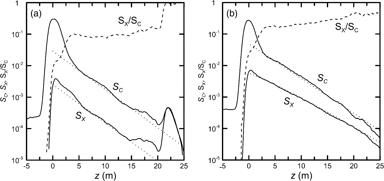 The use of circular polarization can produce larger depolarization ratios, but no additional information. For backscattering (at 180 deg) from a collection of particles with mirror symmetry, van de Hulst used symmetry arguments to show that the Mueller matrix would be diagonal.47 It was later shown that these diagonal elements were related as48,49 where is the unpolarized volume backscatter coefficient at 180 deg and is the single polarization parameter, which has been described49 as “a measure of the propensity of the scattering medium to depolarized the incident polarization.” This implies that the depolarization of an initially polarized beam will be where the first letter in the subscript refers to the co- () or cross-polarized () signal and the second to linear () or circularization (). Because there is only one parameter related to depolarization, however, the contrast between large scattering particles and the background scattering level is the same whether linear or circular polarization is used;49 this has been verified experimentally.50Thus, the quasi-single-scattering approximation can be applied to polarized lidar, with the general result that the information content is the same whether linear or circular polarization is used. However, Eq. (12) shows that the signal level in the cross-polarized channel will be greater when circular polarization is used, which implies a higher signal-to-noise ratio. 3.3.Laser SafetyOceanographic lidars operate with intense pulses of visible light, and ocular safety must be considered. The single-pulse exposure limit is .51 For a typical pulse energy of 100 mJ, this implies that the laser spot diameter needs to be to be safe for direct viewing. To calculate the exposure for light reflected from the surface, the Fresnel reflection coefficient and the surface roughness should be included.52 For exposure to multiple pulses, the exposure limit should be reduced by , where is the number of pulses. For an airborne system, is unlikely to be more than two or three as the illumination moves swiftly. For a lidar on a ship, is generally taken as the number of pulses within the aversion response time of 0.25 s. Where the exposure would be above the limit, access must be limited or protective eyeware used. Often, this can be accomplished by an observer who can stop laser transmission if someone is about to come into the danger zone. For low-level flights of the NOAA lidar, the system is designed to be eyesafe at the sea surface, and the pilot is provided with a remotely controlled laser shutter to use in the event of aircraft below the flight altitude. Marine mammals in the study area present another set of issues. There are regulations for both ship and aircraft operations to prevent harassment of marine mammals. Marine mammals are less susceptible to ocular damage than humans,53 so a system that is eyesafe at the surface according to the standards will not cause damage to marine mammals. Note that this information is provided as a general overview and is not a substitute for a thorough analysis based on published standards such as ANSI Z136.1 (Ref. 54) and Z136.6 (Ref. 55). 4.Applications4.1.FisheriesThe advantages of airborne lidar for fisheries surveys are that large areas can be covered quickly (before the fish move) and at lower cost than with a surface vessel.23 The feasibility of detecting fish schools with an airborne lidar was studied in 1974.56 As early as 1976, an U.S. Navy airborne lidar was used to detect fish south of Florida.57 The next year, the same system measured vertical profiles of fish schools off New Jersey.57 A ship-based lidar was used to detect fish in cages in 1978.58 This early work demonstrated that lidar could be useful for fisheries applications, and this has been confirmed by several subsequent analyses.32,59,60 The easiest case is when large fish are widely separated, so individuals can be seen in the return and counted. As an example, Fig. 4 presents the depths and positions of 69 individual fish that were detected using the cross-polarized lidar signal at night off the Oregon coast.61 During the day, only two individual fish were detected along the identical flight track, suggesting a species that is at depth during the day and near the surface at night. No fish were detected within the cold water of the upwelling zone within 40 km of the coast. These characteristics suggest that most of these fish are likely albacore tuna (Thunnus alalunga). The density of fish detected beyond the upwelling zone during this survey was , where the uncertainty was estimated assuming a random distribution of fish within the survey area. Fig. 4Depth, , and position, (km from the coastline along 46°N latitude), of individual fish detected (symbols). Line is sea-surface temperature, , measured by an infrared radiometer on the same aircraft. 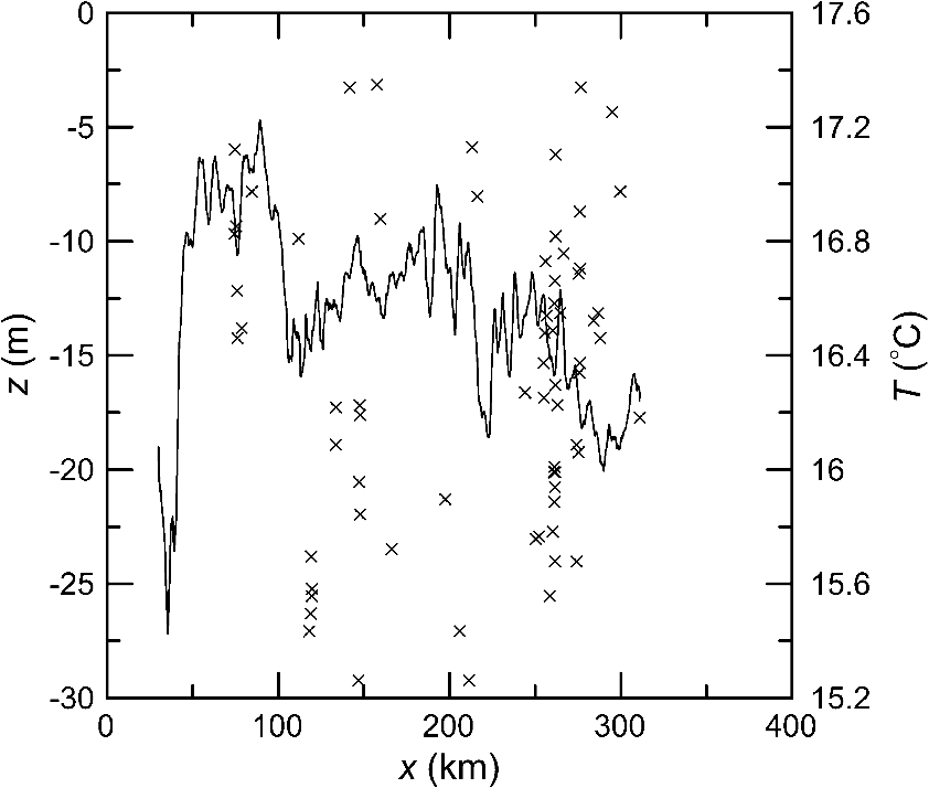 More work has been done on the harder problem of quantitative estimates of populations of schooling fish species, where many individuals are within the illuminated region for each shot. In this case, we note that in Eq. (1) is the sum of a fish component, , and a water component, , which includes everything else. To estimate , we have to filter the data in some way to separate the two components. Depending on conditions, we can assume that the water component does not vary with depth or that it has some depth profile that does not vary horizontally over some distance that is large compared with the horizontal extent of the fish schools.23 In either case, we can apply a filter and a threshold to remove small signals to estimate and . To increase the contrast between the fish and water components, the cross-polarized component is generally used. The technique of applying a filter and threshold is then used to obtain , where is the cross-polarized fraction of the return from fish. Figure 5 shows an example for a school of sardines (Sardinops sagax) observed by airborne lidar.61 Fig. 5Calibrated cross-polarized lidar return, (values in according to the color bar on the right), from a school of sardines versus depth, , and distance along the flight track, . Inset is section of raw lidar data before correction for attenuation and calibration.61 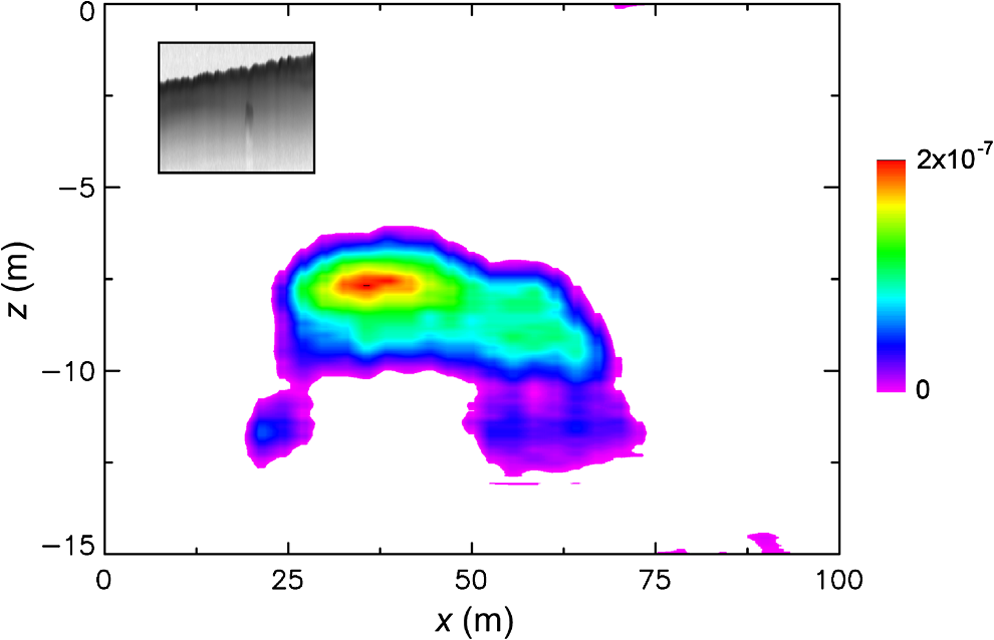 There have been a number of validation tests to establish a correlation between lidar results and traditional acoustic and trawl techniques using a relative value of instead of an absolute value. The correlation approach is attractive because it does not require absolute calibration of the lidar or target strength estimates of the fish species involved. It does require estimation of, and correction for, attenuation. When individual schools were identified visually and targeted by both lidar and acoustics, the correlation was very high (0.994).62 Comparisons have also been made using data from the same area, but taken at different times. In these cases, correlations with acoustics24,63 and with trawls61,64 were both lower, but as long as the time difference was less than four days and appropriate filtering and threshold values were applied. A more difficult step is to convert an absolute value for into a biomass estimate. This requires calibration of the lidar to get the absolute value of and estimates of the target strength and average mass of the target species. The biomass density () can be found from where is the mass of an individual fish, is the cross-sectional area of a single fish, and is the cross-polarized fraction of the average bidirectional reflectance distribution function of a single fish for polarized lidar illumination, measured at the lidar observation angle. The product is target strength, which has been measured for several species of dead fish.65,66 More reliable measurements have been made using live sardines,20 mackerel,67 and menhaden.68Similar techniques have been used to detect large zooplankton, although the details of filtering and the thresholds used are different. With appropriate processing, a correlation of 0.78 was obtained between lidar and acoustic measurements of copepods in Prince William Sound, Alaska.69 In addition to biomass estimates for fisheries management, lidar can be used to investigate aspects of fish behavior. For example, lidar data were used with those from an infrared radiometer on the same aircraft to show that sardines were associated with thermal fronts in the NE Pacific Ocean,70 validating an earlier prediction.71 Lidar data were used with visual observations to show the evolution of a foraging event involving whales, seabirds, herring, and euphasiids in the SE Bering Sea.72 Evidence that fish near the surface avoid research vessels that are trying to measure their abundance has also been observed, in agreement with other methods.73 4.2.Scattering LayersLidar is also able to profile optical scattering layers in the upper ocean, whether operating from a ship74 or aircraft.75 Most of these layers are phytoplankton and comprise large, nonspherical algal cells. Individual cells can be longer than 1 mm, and multicell colonies even larger. The structures can be very complex, which results in high-order multiple scattering within individual cells. As a result, these layers are more detectable in the cross-polarized return of a polarized lidar than in the copolarized return or in an unpolarized lidar.32,76,77 Of particular importance are thin plankton layers,78–81 in which high concentrations of nutrients and phytoplankton are found in a thin layer often associated with the pycnocline. These layers can be as little as 10 cm thick, yet extend for km and persist for days. These concentrated layers can affect the biogeochemical processes in the upper ocean, including primary productivity and the formation of harmful algal blooms. Airborne lidar data were used to investigate the occurrence of thin layers and mechanisms of formation,77 with the result that layers were found to be associated with wind-driven and topographic upwelling, fresh-water influx, and warm core eddies. Figure 6 shows an example of a plankton layer within a warm-core (anticyclonic) eddy in the Gulf of Alaska.77 The mechanism for the productivity of warm-core eddies is an area of active investigation,82,83 and the discovery of thin layers on the scale shown in the figure may provide important information. Fig. 6Thin plankton layer within a warm-core eddy in the Gulf of Alaska versus depth, , and distance along the flight track, . Data are uncalibrated, but relative values follow the same color scale as Fig. 5. (Reproduced from Ref. 77) 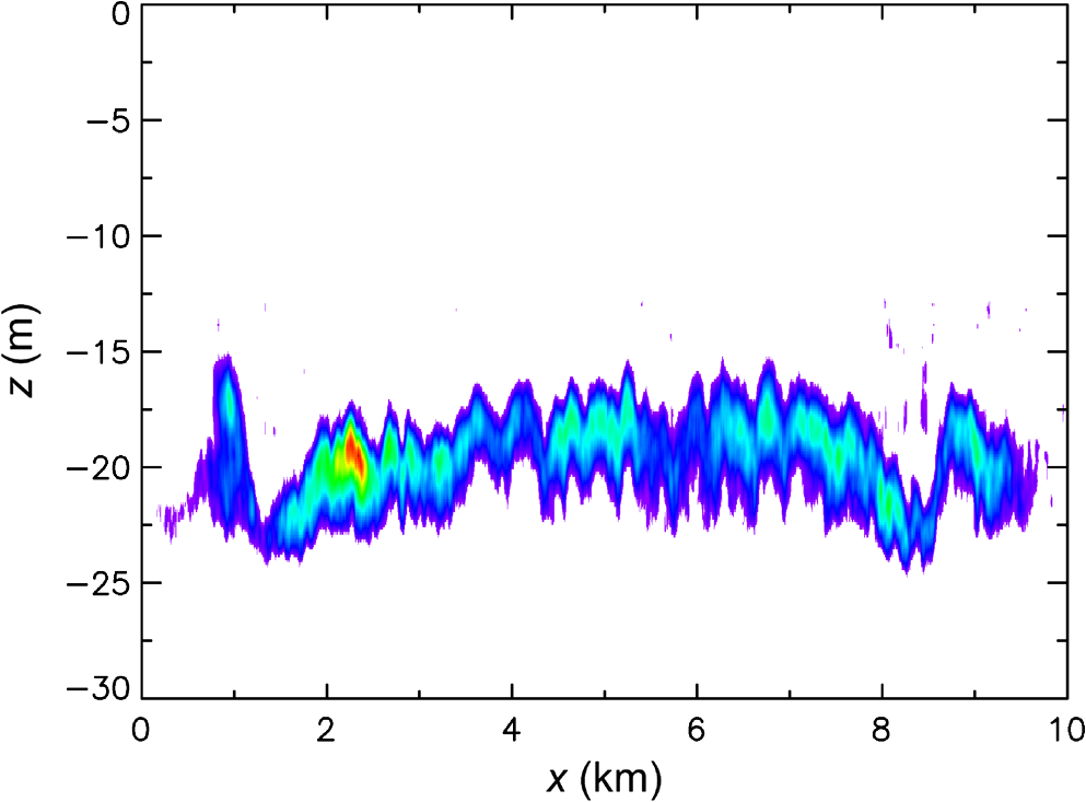 Plankton layers also affect retrievals based on passive optical measurements.84,85 Comparisons between lidar measurements, in-situ measurements, and the statistics of variability in passive measurements have been used to investigate some of these effects.86,87 4.3.Optical PropertiesAnother application of lidar is the inference of the optical properties of sea water, at least at the laser wavelength. From Eq. (1), it is evident that two properties of the water contribute to the signal—the lidar attenuation and the volume backscattering coefficient, so the problem is ill posed and suitable inversion techniques must be applied. The most common technique in atmospheric lidar is to assume a value for the ratio , known as the lidar ratio. This ratio will change with the type of scatterers, but is relatively unaffected by changes in number density or atmospheric absorption (negligible at common lidar wavelengths). For example, six aerosol types are defined for the cloud-aerosol lidar and infrared pathfinder satellite observations (CALIPSO) lidar, and a fixed lidar ratio is used for each.88 The variety of scattering particles in the ocean is much larger, however, so measuring the lidar ratio for each type is not a practical approach. Although sophisticated inversion techniques have been developed for atmospheric lidar, the same cannot be said for oceanographic lidar retrievals. Where the optical properties are not changing with depth, as in a surface mixed layer, the lidar signal will exhibit an exponential decrease with depth (e.g., Fig. 3). The lidar attenuation is easily estimated from the slope of that decrease, even for an uncalibrated system.46,89 Generally, the attenuation of the lidar signal is between the beam attenuation, , and the diffuse attenuation, , as expected from the discussion in Sec. 3.28,31,90,91 This suggests that either or both of the attenuation coefficients could be inferred with the appropriate lidar geometry. It may also be possible to infer the absorption coefficient from the lidar attenuation coefficient by considering the relationship between volume backscatter and attenuation in a particular area. A linear relationship between attenuation and backscattering, as in Fig. 7, would suggest that the absorption coefficient can be estimated from the limiting lidar attenuation with no backscatter.46 Intercept values are 0.27, 0.12, and for the Columbia River plume, near-shore water outside of the plume, and offshore water, respectively. These values are about what would be expected for absorption coefficient at 532 nm, although direct comparisons of lidar and in-situ measurements are needed to confirm the relationship. This example was only done for the near-surface layer, but there is no reason that the technique cannot be extended to obtain profiles of absorption coefficient. Fig. 7Lidar attenuation coefficient, , as a function of the uncalibrated volume backscatter function, , near the surface for offshore (+) and nearshore (•) waters. Lines are regressions to the corresponding data outside (solid) and inside (dashed) the Columbia River plume. (Reproduced from Ref. 46) 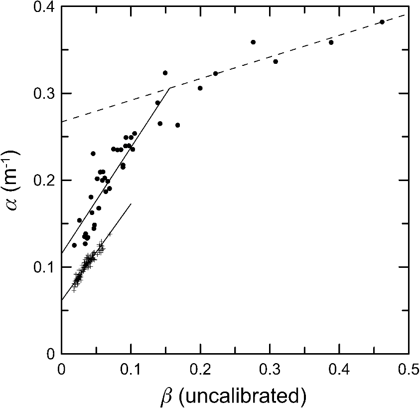 One reason for interest in the absorption coefficient is that it can provide a measure of the amount of dissolved organic material in milligrams of carbon per liter (). The specific absorption coefficient is defined as the absorption coefficient per unit of dissolved organic material. Using a value of for the specific absorption coefficient at 450 nm (Ref. 92) and converting to 532 nm (Ref. 91), we get a specific absorption coefficient at the lidar wavelength of . Removing the clear-water absorption from the estimated Columbia River plume absorption and dividing by this specific absorption provides an estimate of . Recent measurements in the river have reported values of ,93 suggesting this might be a viable technique. The estimated uncertainty in the specific absorption coefficient is (Ref. 92), however, and more measurements of this quantity are needed. There are two scattering parameters that are typically of interest—the scattering coefficient, , and the backscattering coefficient . With measured values for and , as above, the scattering coefficient can be obtained from . The backscatter coefficient, of interest to remote sensing, is more difficult. However, the particulate volume scattering function normalized by seems to have a fairly consistent shape for scattering angles between 90 and 170 deg.94 This shape, based on three million measurements at 10 locations, was approximated by a fourth-order polynomial in Ref. 94, which can be extrapolated to a scattering angle of 180 deg. The result is that the particulate contribution can be estimated from the lidar measurement of using the relationship where the constant within the square brackets is for pure sea water at 532 nm. The total is this value plus the pure water value of .4.4.Upper Ocean DynamicsThe dynamics of the upper ocean are rather complex.95 There is an ever-shifting balance between stratification and vertical mixing. Stratification is enhanced by solar heating of the surface and by fresh-water influx from terrestrial runoff and melting ice. Mixing is enhanced by winds, wind-induced currents, tidal currents, and turbulence. The result is often an upper mixed layer with a density gradient, or pycnocline, at the bottom. The frequent association of plankton layers with the pycnocline78 implies that the pycnocline depth can often be mapped by lidar.77 Although most of these effects are local, internal waves caused by the interaction of tidal currents and bottom topography can propagate long distances on the pycnocline and produce mixing far from the source.96,97 When plankton layers are present at the pycnocline, internal waves propagating on the pycnocline can be detected by lidar, and internal-wave observations have been reported by ship-based74,98 and airborne lidars.50,77,99 Large, nonlinear internal waves are easy to distinguish in lidar data, as in the example (Fig. 8) from airborne lidar in West Sound, Orcas Island, Washington.50 The characteristics of these waves measured by the lidar can be used to infer characteristics of the mixed layer. To do this, the assumption is made that the density structure in the ocean can be approximated by two layers of different density with a scattering layer at the boundary. The thickness of the upper layer is obtained directly from the lidar, and the thickness of the lower layer is obtained from the total water depth provided by navigational charts. The amplitude of the wave is also directly measured by the lidar. More information requires a second pass of the lidar, so the propagation speed of the wave can be inferred. For a weakly nonlinear wave, the Korteweg–de Vries equation can be used to obtain the density difference between the upper and lower layers.50 Combining this information, the total energy density within an internal-wave packet can be estimated.50 In addition to the obvious nonlinear internal wave packets, the ocean has a random background field of weak internal waves that depend on wavenumber, , as ,100 and this has also been observed by lidar.77 Fig. 8Scattering layer depth, , along 300 m of flight track, . Internal wave has wavelength of 50 m and amplitude of 2 m.50 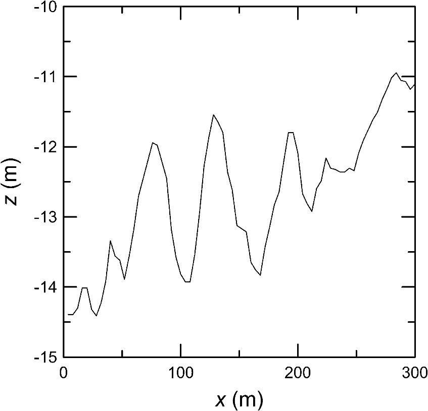 The power spectrum of lidar backscatter also provides some insight into turbulent processes. For homogeneous, isotropic turbulence, the distribution of a passive tracer would be expected to have a power spectrum. With few exceptions, phytoplankton drift with the local current and can be treated as a passive tracer, independent of their size and shape. Thus, lidar signal fluctuations would be expected to have a power spectrum when the distribution of phytoplankton is affected by turbulence. Lidar measurements of backscatter at constant depth in the NE Pacific Ocean, however, produced a spectral slope that was lower at .101 The reason for the difference seems to be that this part of the ocean is not homogeneous, but stratified. Under these conditions, one would expect to find the slope along a line of constant density, not constant depth,102,103 and this was observed in the lidar fluctuations along the center of a plankton layer.50 4.5.BubblesBubbles near the surface of the ocean, produced by breaking waves, affect a number of important processes. They facilitate the exchange of gases between the atmosphere and ocean104–106 and the production of cloud-condensing aerosols in the atmosphere.107,108 They produce sound in the ocean109 and affect its propagation.110,111 Bubbles also scatter light, and the resulting change in ocean color can affect estimates of chlorophyll concentration based on the color of scattered light.112–114 While most of the bubbles are in the top 1 to 2 m of the ocean, breaking waves can produce plumes extending down to 20 m.115 The lidar return from bubbles has been theoretically estimated using Monte-Carlo simulation116,117 and geometric optics.118 The copolarized lidar return has been shown to be proportional to the total volume of air within the illuminated region, independent of the bubble size distribution as long as the bubbles are spherical and the density is low enough that multiple scattering can be neglected. A linear dependence of lidar signal on bubble number concentration has been verified in the laboratory.119 This suggests that a copolarized lidar receiver can provide profiles of bubble void fraction important to studies of air/sea gas exchange processes. The utility of lidar for ship-wake measurements has been demonstrated in the laboratory,120 and wakes have been detected in the open ocean. Figure 9 is an example of the lidar return from the surface along a flight track that crossed the wakes of two boats, observed during a fisheries survey in Chesapeake Bay.68 A photo of the surface shows the lidar track crossing two wakes. The stronger one (closer to the passage of the boat) shows the three lobes characteristic of the propeller wake and two hull wakes. In this case, the signal is partially depolarized by some combination of scattering from large, nonspherical bubbles and multiple scattering from the dense bubble cloud. In the weaker wake (farther behind the boat), the depolarization is too small to be detected. By this time, the larger bubbles have risen to the surface and the bubble density is lower. Fig. 9Plot of fraction of lidar volume scattering coefficient, , for copolarized (solid line) and cross-polarized (dashed line) returns from the surface as functions of position along the flight track, , over two boat wakes. The track in the plot follows the black line in the photo of the wakes from bottom to top. 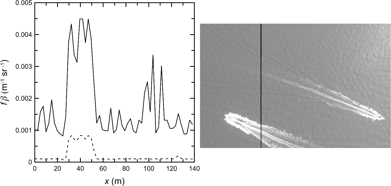 5.Future Directions5.1.Ocean Lidar RatioTo date, techniques to simultaneously retrieve attenuation and scattering from lidar profiles have been limited to cases where these properties of the water column are slowly varying with depth. Figure 7 suggests that the particulate component of the lidar ratio for the ocean might be constant for a number of broad classes of water types, even though the actual value is not. The figure shows that the slopes are similar for both near-shore and offshore water outside of the Columbia River plume, whereas there is a different slope within the plume. If the intercept of the line (the absorption) is subtracted from the data, this produces one value of the lidar ratio within the plume and another outside of it. More studies of the lidar ratio for different water types can be expected in the future, both to improve lidar retrievals and to characterize different water types. 5.2.TemperatureTwo different techniques have been investigated for temperature profiling in the ocean using inelastic scattering. Raman scattering excites a vibrational mode of the water molecule, which produces a frequency shift toward longer wavelengths over a broad band between 3000 and . Brillouin scattering is from acoustic pressure fluctuations in the water and is Doppler shifted both up and down in frequency in a narrow frequency band at 7.5 GHz (). The scattering strength for these two processes, however, is for both.121 Neither of these are new concepts, but the component technologies have not been suitable for widespread open-ocean application. The Raman scattering approach uses the fact that water comprises clusters of molecules that are weakly bound (polymer form) and independent molecules (monomer form) whose relative concentrations are in thermodynamic equilibrium. As temperature increases, order decreases and the balance shifts toward a higher concentration of monomers. The Raman shift of the two forms are different—peaks at 3535 and are from monomeric water and increase with increasing temperature, while peaks at 3247 and are from polymeric water and decrease with increasing temperature.122 Thus, the ratio of the Raman return at two wavelengths can be used to infer temperature. For 532-nm illumination, one of the Raman-shifted wavelengths would be between the monomer peaks at 655 and 659 nm, and the other would be between the polymer peaks at 643 and 651 nm. Another difference between Raman scattering from monomer and polymer waters is that the former is not depolarized for polarized illumination, while the latter is. This implies that depolarization of the Raman signal can also be used to infer temperature. Because the Raman-shifted light is strongly absorbed when 532-nm illumination is used, measurements have used shorter-wavelength lasers123–126 unless only near-surface values are required.127,128 Using this technique, temperature profiles have been measured to 30 m using a 450-nm laser on a ship.123 However, the technique has not found wide application largely because of interference with background light over the broad Raman band, distortion of the spectrum by differential absorption over that same band, and practical problems associated with high-energy blue sources. The frequency of the Brillouin return provides a measure of the speed of sound in the water, , which depends on temperature, salinity, and pressure as129 where is temperature (°C), is salinity (PSU), and is pressure (). Over the range of values typical of the upper 100 m of the ocean (, , ), changes by , changes by , and changes by . A complicated combined term changes by , and is not reproduced here. can be estimated from depth, so temperature can be estimated from sound speed within a few percent by assuming an average salinity and neglecting . The lidar Doppler shift for 532-nm laser light and a sound speed of is 7.5 GHz, which is typically measured with an interferometer. An accuracy of 1°C implies a frequency measurement with 20 MHz accuracy, requiring very precise optical interferometers.Most of the work on ocean temperature sensing by Brillouin lidar has been theoretical analyses130–132 or laboratory demonstrations,133–135 as described in another paper in this issue.136 It has not found widespread application because the required laser stability and receiver frequency accuracy have been difficult to obtain outside of the laboratory. These are both areas of active research,136–139 and the application of lidar profiling of temperature in the open ocean can be expected in the future.136 5.3.High-Spectral-Resolution LidarThe concept of a high-spectral-resolution lidar (HSRL) originated as a way to separate aerosol from molecular scattering in the atmosphere,140–142 based on the premise that the Doppler shift from aerosols is small compared with that from air molecules. This same concept can be applied to sea water in order to simultaneously measure attenuation and backscattering using a two-channel receiver.143 The volume backscatter coefficient of pure seawater, , can be calculated precisely, since the density of water changes very little in the upper 50 to 100 m. Over 98% of this scattered light is in the two symmetric Brillouin peaks Doppler shifted up or down by 7.5 GHz (7 pm for an initial wavelength of 532 nm).144 The Doppler shift from particulate scattering is very small, so one of the two receiver channels is equipped with a spectral filter that only passes the Brillouin peaks. The signal from this channel is inverted using Eq. (1), with , to obtain . The other receiver channel responds to both seawater and particulate scattering. The signal from this channel is inverted using , obtained from the Brillouin channel, in Eq. (1) to obtain , which, for this channel, is the sum of seawater and particulate components. An optical filter to pass the Brillouin return is much simpler than an interferometer to precisely measure its frequency, so the application of HSRL to measure attenuation and scattering in the ocean can be expected earlier than temperature profiling using the Brillouin technique. 5.4.Space-Based LidarThe cloud-aerosol lidar with orthogonal polarization on the CALIPSO satellite was launched to study clouds and aerosols in the atmosphere,145 but has co- and cross-polarized receivers for the 532-nm laser light. This similarity has motivated several studies into possible ocean subsurface returns.146,147 However, the range-resolution of this lidar was designed with atmospheric studies in mind. Near the surface, the sample frequency is 5 MHz, which corresponds to a range resolution of 22.5 m in water. Prior to sampling, the signal has been low-pass filtered with a 2-MHz filter, so the strong surface return extends over three samples. In addition, the photomultipliers have a slowly decaying tail from signal-induced fluorescence within the tubes.148 The result of these two effects is an impulse-response function given by149 for the unpolarized and cross-polarized receiver channels, respectively. These two effects mask the subsurface return under most conditions.Despite these limitations, there is evidence of subsurface return in the cross-polarized lidar channel at the two sample depths of 28 and 50 m,149 and it seems feasible to build a space-based lidar with depth resolution of a meter or so, better matched to oceanographic requirements.150,151 Coupled with ocean color measurements, this would be a powerful tool for global observations of the upper ocean. 6.ConclusionsThis paper has described the characteristics of the critical lidar components that need to be considered in the design. For many applications, Q-switched, frequency-doubled Nd:YAG will be the clear choice for a laser, in no small part because of its reliable operation in the field. For open-ocean applications, a blue laser would provide better depth penetration, but the technology is more complex. The two receiver characteristics that must be carefully considered are field of view and dynamic range. For many applications, a wider field of view will be desired to minimize the attenuation of the signal with depth, even though this will result in increased levels of background light. There are several approaches to maximizing dynamic range, all of which have advantages and disadvantages. The eventual solution will be a high-speed digitizer with sufficient dynamic range, and this is probably not too far off. This paper has described the basic equations describing the performance of profiling lidars. Because of its simplicity, the quasi-single-scattering approximation is the best choice for many applications. The extension of this theoretical approach to include polarization was also described. This extension led to the conclusion that linear and circular polarizations are equivalent in the information content, but circular polarization might be better from a signal-to-noise consideration. This paper has described applications of lidar for profiling several properties of the upper ocean. These properties include the vertical distribution of fish, plankton, bubbles, and the optical properties of scattering, absorption, and attenuation that are affected by suspended sediments and dissolved substances. Lidar has also been shown to be useful in understanding the dynamical properties of the upper ocean. Scattering particles move with the water and act as tracers for mixing processes like internal waves and turbulence. They are also often associated with the pycnocline, which identifies the depth of the oceanic mixed layer. The conclusion was that a great deal of information about the upper ocean can be obtained from lidar systems. This information has relevance to physical, biological, and chemical oceanography. This paper has described several areas where progress in lidar profiling can be expected in the future. Quantitative retrievals of atmospheric lidars have been improved by applications of HSRL techniques and by thorough investigations of the lidar ratio in different atmospheric conditions. These same techniques will be applied to oceanographic lidars, and similar progress is expected. Technological advances, especially in the area of stable lasers and filters, are likely to lead to practical application of lidar temperature profiling. Farther into the future, global coverage from an oceanographic lidar operating from a satellite is likely. ReferencesC. R. McClain,
“A decade of satellite ocean color observations,”
Ann. Rev. Mar. Sci., 1
(1), 19
–42
(2009). http://dx.doi.org/10.1146/annurev.marine.010908.163650 1941-1405 Google Scholar
D. A. Siegelet al.,
“Regional to global assessments of phytoplankton dynamics from the SeaWiFS mission,”
Remote Sens. Environ., 135 77
–91
(2013). http://dx.doi.org/10.1016/j.rse.2013.03.025 RSEEA7 0034-4257 Google Scholar
M. J. BehrenfeldP. G. Falkowski,
“Photosynthetic rates derived from satellite-based chlorophyll concentration,”
Limnol. Oceanogr., 42
(1), 1
–20
(1997). http://dx.doi.org/10.4319/lo.1997.42.1.0001 LIOCAH 0024-3590 Google Scholar
T. Westberryet al.,
“Carbon-based primary productivity modeling with vertically resolved photoacclimation,”
Global Biogeochem. Cycles, 22
(2), GB2024
(2008). http://dx.doi.org/10.1029/2007GB003078 GBCYEP 0886-6236 Google Scholar
J. Busck,
“Underwater 3-D optical imaging with a gated viewing laser radar,”
Opt. Eng., 44
(11), 116001
(2005). http://dx.doi.org/10.1117/1.2127895 OPEGAR 0091-3286 Google Scholar
B. CochenourL. MullenJ. Muth,
“Modulated pulse laser with pseudorandom coding capabilities for underwater ranging, detection, and imaging,”
Appl. Opt., 50
(33), 6168
–6178
(2011). http://dx.doi.org/10.1364/AO.50.006168 APOPAI 0003-6935 Google Scholar
J. H. ChurnsideJ. J. Wilson,
“Airborne lidar imaging of salmon,”
Appl. Opt., 43
(6), 1416
–1424
(2004). http://dx.doi.org/10.1364/AO.43.001416 APOPAI 0003-6935 Google Scholar
G. C. GuentherM. W. BrooksP. E. LaRocque,
“New capabilities of the ‘SHOALS’ airborne lidar bathymeter,”
Remote Sens. Environ., 73
(2), 247
–255
(2000). http://dx.doi.org/10.1016/S0034-4257(00)00099-7 RSEEA7 0034-4257 Google Scholar
C. W. FinklL. BenedetJ. L. Andrews,
“Submarine geomorphology of the continental shelf off southeast Florida based on interpretation of airborne laser bathymetry,”
J. Coastal Res., 21
(6), 1178
–1190
(2005). http://dx.doi.org/10.2112/05A-0021.1 JCRSEK 0749-0208 Google Scholar
J. A. Yoderet al.,
“Spatial variability in near-surface chlorophyll a fluorescence measured by the airborne oceanographic lidar (AOL),”
Deep Sea Res. Part 2 Top. Stud. Oceanogr., 40
(1–2), 37
–53
(1993). http://dx.doi.org/10.1016/0967-0645(93)90005-8 DSROEK 0967-0645 Google Scholar
I. Leiferet al.,
“State of the art satellite and airborne marine oil spill remote sensing: application to the BP deepwater horizon oil spill,”
Remote Sens. Environ., 124 185
–209
(2012). http://dx.doi.org/10.1016/j.rse.2012.03.024 RSEEA7 0034-4257 Google Scholar
A. ChekalyukM. Hafez,
“Advanced laser fluorometry of natural aquatic environments,”
Limnol. Oceanogr. Methods, 6
(11), 591
–609
(2008). http://dx.doi.org/10.4319/lom.2008.6.591 1541-5856 Google Scholar
Y. Huet al.,
“Sea surface wind speed estimation from space-based lidar measurements,”
Atmos. Chem. Phys., 8
(13), 3593
–3601
(2008). http://dx.doi.org/10.5194/acpd-8-2771-2008 1680-7367 Google Scholar
J. A. ShawJ. H. Churnside,
“Scanning-laser glint measurements of sea-surface slope statistics,”
Appl. Opt., 36
(18), 4202
–4213
(1997). http://dx.doi.org/10.1364/AO.36.004202 APOPAI 0003-6935 Google Scholar
C. Flamantet al.,
“Analysis of surface wind and roughness length evolution with fetch using a combination of airborne lidar and radar measurements,”
J. Geophys. Res., 108
(C3), 8058
(2003). http://dx.doi.org/10.1029/2002JC001405 JGREA2 0148-0227 Google Scholar
A. Morel,
“Light and marine photosynthesis: a spectral model with geochemical and climatological implications,”
Prog. Oceanogr., 26
(3), 263
–306
(1991). http://dx.doi.org/10.1016/0079-6611(91)90004-6 POCNA8 0079-6611 Google Scholar
C. D. Mobley, Light and Water: Radiative Transfer in Natural Waters, Academic Press, San Diego
(1994). Google Scholar
A. BricaudA. MorelL. Preiur,
“Absorption by dissolved organic matter of the sea (yellow substance) in the UV and visible domains,”
Limnol. Oceanogr., 26
(1), 43
–53
(1981). http://dx.doi.org/10.4319/lo.1981.26.1.0043 LIOCAH 0024-3590 Google Scholar
C. S. RoeslerM. J. PerryK. L. Carder,
“Modeling in situ phytoplankton absorption from total absorption spectra in productive inland marine waters,”
Limnol. Oceanogr., 34
(8), 1510
–1523
(1989). http://dx.doi.org/10.4319/lo.1989.34.8.1510 LIOCAH 0024-3590 Google Scholar
J. H. ChurnsideJ. J. WilsonV. V. Tatarskii,
“Lidar profiles of fish schools,”
Appl. Opt., 36
(24), 6011
–6020
(1997). http://dx.doi.org/10.1364/AO.36.006011 APOPAI 0003-6935 Google Scholar
M. P. Bristow,
“Lidar-signal compression by photomultiplier gain modulation: influence of detector nonlinearity,”
Appl. Opt., 37
(27), 6468
–6479
(1998). http://dx.doi.org/10.1364/AO.37.006468 APOPAI 0003-6935 Google Scholar
M. H. Sweet,
“A logarithmic photo-multiplier tube photo-meter,”
J. Opt. Soc. Am., 37
(6), 432
–432
(1947). http://dx.doi.org/10.1364/JOSA.37.000432 JOSAAH 0030-3941 Google Scholar
J. H. ChurnsideJ. J. Wilson,
“Airborne lidar for fisheries applications,”
Opt. Eng., 40
(3), 406
–414
(2001). http://dx.doi.org/10.1117/1.1348000 OPEGAR 0091-3286 Google Scholar
P. Carreraet al.,
“Comparison of airborne lidar with echosounders: a case study in the coastal Atlantic waters of southern Europe,”
ICES J. Mar. Sci., 63
(9), 1736
–1750
(2006). http://dx.doi.org/10.1016/j.icesjms.2006.07.004 ICESEC 1054-3139 Google Scholar
G. P. KokhanenkoI. E. PennerV. S. Shamanaev,
“Expanding the dynamic range of a lidar receiver by the method of dynode-signal collection,”
Appl. Opt., 41
(24), 5073
–5077
(2002). http://dx.doi.org/10.1364/AO.41.005073 APOPAI 0003-6935 Google Scholar
M. G. LöfdahlV. M. J. HenriquesD. Kiselman,
“A tilted interference filter in a converging beam,”
Astron. Astrophys., 533 A82
(2011). http://dx.doi.org/10.1051/0004-6361/201117305 AAEJAF 0004-6361 Google Scholar
W. W. GreggK. L. Carder,
“A simple spectral solar irradiance model for cloudless maritime atmospheres,”
Limnol. Oceanogr., 35
(8), 1657
–1675
(1990). http://dx.doi.org/10.4319/lo.1990.35.8.1657 LIOCAH 0024-3590 Google Scholar
J. H. Leeet al.,
“Oceanographic lidar profiles compared with estimates from in situ optical measurements,”
Appl. Opt., 52
(4), 786
–794
(2013). http://dx.doi.org/10.1364/AO.52.000786 APOPAI 0003-6935 Google Scholar
J. L. BuftonF. E. HogeR. N. Swift,
“Airborne measurements of laser backscatter from the ocean surface,”
Appl. Opt., 22
(17), 2603
–2618
(1983). http://dx.doi.org/10.1364/AO.22.002603 APOPAI 0003-6935 Google Scholar
G. W. KattawarG. N. Plass,
“Time of flight lidar measurements as an ocean probe,”
Appl. Opt., 11
(3), 662
–666
(1972). http://dx.doi.org/10.1364/AO.11.000662 APOPAI 0003-6935 Google Scholar
H. R. Gordon,
“Interpretation of airborne oceanic lidar: effects of multiple scattering,”
Appl. Opt., 21
(16), 2996
–3001
(1982). http://dx.doi.org/10.1364/AO.21.002996 APOPAI 0003-6935 Google Scholar
M. M. Krekovaet al.,
“Numerical evaluation of the possibilities of remote laser sensing of fish schools,”
Appl. Opt., 33
(24), 5715
–5720
(1994). http://dx.doi.org/10.1364/AO.33.005715 APOPAI 0003-6935 Google Scholar
G. M. KrekovM. M. KrekovaV. S. Shamanaev,
“Laser sensing of a subsurface oceanic layer. I. Effect of the atmosphere and wind-driven sea waves,”
Appl. Opt., 37
(9), 1589
–1595
(1998). http://dx.doi.org/10.1364/AO.37.001589 APOPAI 0003-6935 Google Scholar
G. M. KrekovM. M. KrekovaV. S. Shamanaev,
“Laser sensing of a subsurface oceanic layer. II. Polarization characteristics of signals,”
Appl. Opt., 37
(9), 1596
–1601
(1998). http://dx.doi.org/10.1364/AO.37.001596 APOPAI 0003-6935 Google Scholar
R. E. Walker, Marine Light Field Statistics, John Wiley and Sons, New York
(1994). Google Scholar
K. Stamneset al.,
“Numerically stable algorithm for discrete-ordinate-method radiative transfer in multiple scattering and emitting layered media,”
Appl. Opt., 27
(12), 2502
–2509
(1988). http://dx.doi.org/10.1364/AO.27.002502 APOPAI 0003-6935 Google Scholar
K. I. Gjerstadet al.,
“Monte Carlo and discrete-ordinate simulations of irradiances in the coupled atmosphere-ocean system,”
Appl. Opt., 42
(15), 2609
–2622
(2003). http://dx.doi.org/10.1364/AO.42.002609 APOPAI 0003-6935 Google Scholar
K. MitraJ. H. Churnside,
“Transient radiative transfer equation applied to oceanographic lidar,”
Appl. Opt., 38
(6), 889
–895
(1999). http://dx.doi.org/10.1364/AO.38.000889 APOPAI 0003-6935 Google Scholar
M. ChamiR. SanterE. Dilligeard,
“Radiative transfer model for the computation of radiance and polarization in an ocean-atmosphere system: polarization properties of suspended matter for remote sensing,”
Appl. Opt., 40
(15), 2398
–2416
(2001). http://dx.doi.org/10.1364/AO.40.002398 APOPAI 0003-6935 Google Scholar
P.-W. Zhaiet al.,
“A vector radiative transfer model for coupled atmosphere and ocean systems based on successive order of scattering method,”
Opt. Express, 17
(4), 2057
–2079
(2009). http://dx.doi.org/10.1364/OE.17.002057 OPEXFF 1094-4087 Google Scholar
L. S. DolinV. A. Saveliev,
“Backscattering signal in pulsed irradiation of a turbid medium with a narrow, directional light beam,”
Izvestiya Akademii Nauk SSSR seriya Fizika Atmosfery i Okeana, 7
(5), 505
–510
(1971). Google Scholar
I. L. Katsevet al.,
“Efficient technique to determine backscattered light power for various atmospheric and oceanic sounding and imaging systems,”
J. Opt. Soc. Am. A, 14
(6), 1338
–1346
(1997). http://dx.doi.org/10.1364/JOSAA.14.001338 JOAOD6 0740-3232 Google Scholar
H. R. Gordon,
“Simple calculation of the diffuse reflectance of the ocean,”
Appl. Opt., 12
(12), 2803
–2804
(1973). http://dx.doi.org/10.1364/AO.12.002803 APOPAI 0003-6935 Google Scholar
H. R. Gordon,
“Can the Lambert-Beer law be applied to the diffuse attenuation coefficient of ocean water?,”
Limnol. Oceanogr., 34
(8), 1389
–1409
(1989). http://dx.doi.org/10.4319/lo.1989.34.8.1389 LIOCAH 0024-3590 Google Scholar
Z.-P. Leeet al.,
“Diffuse attenuation coefficient of downwelling irradiance: an evaluation of remote sensing methods,”
J. Geophys. Res., 110
(C2), C02017
(2005). http://dx.doi.org/10.1029/2004JC002573 JGREA2 0148-0227 Google Scholar
J. H. Churnside,
“Polarization effects on oceanographic lidar,”
Opt. Express, 16
(2), 1196
–1207
(2008). http://dx.doi.org/10.1364/OE.16.001196 OPEXFF 1094-4087 Google Scholar
H. C. van de Hulst, Light Scattering by Small Particles, Dover, New York
(1981). Google Scholar
M. I. MishchenkoJ. W. Hovenier,
“Depolarization of light backscattered by randomly oriented nonspherical particles,”
Opt. Lett., 20
(12), 1356
–1358
(1995). http://dx.doi.org/10.1364/OL.20.001356 OPLEDP 0146-9592 Google Scholar
G. G. Gimmestad,
“Reexamination of depolarization in lidar measurements,”
Appl. Opt., 47
(21), 3795
–3802
(2008). http://dx.doi.org/10.1364/AO.47.003795 APOPAI 0003-6935 Google Scholar
J. H. Churnsideet al.,
“Airborne lidar detection and characterization of internal waves in a shallow fjord,”
J. Appl. Remote Sens., 6
(1), 63611
–63615
(2012). http://dx.doi.org/10.1117/1.JRS.6.063611 1931-3195 Google Scholar
D. SlineyM. Wolbarsht, Safety with Lasers and other Optical Sources, Plenum Press, New York
(1980). Google Scholar
K. M. Hock,
“Probability theory of laser safety at sea,”
Opt. Eng., 35
(4), 1098
–1104
(1996). http://dx.doi.org/10.1117/1.600598 OPEGAR 0091-3286 Google Scholar
H. M. ZornJ. H. ChurnsideC. W. Oliver,
“Laser safety thresholds for cetaceans and pinnipeds,”
Mar. Mammal Sci., 16
(1), 186
–200
(2000). http://dx.doi.org/10.1111/mms.2000.16.issue-1 MMSCEC 0824-0469 Google Scholar
American National Standards Institute, American National Standard for Safe Use of Lasers, 249 Laser Institute of America, Orlando, Florida
(2007). Google Scholar
American National Standards Institute, American National Standard for Safe use of Lasers Outdoors, 116 Laser Institute of America, Orlando, Florida
(2005). Google Scholar
D. L. MurphreeC. D. TaylorR. W. McClendon,
“Mathematical modeling for the detection of fish by an airborne laser,”
AIAA J., 12
(12), 1686
–1692
(1974). http://dx.doi.org/10.2514/3.49579 AIAJAH 0001-1452 Google Scholar
J. L. SquireH. Krumboltz,
“Profiling pelagic fish schools using airborne optical lasers and other remote sensing techniques,”
Mar. Tech. Soc. J., 15
(4), 29
–31
(1981). MTSJBB 0025-3324 Google Scholar
K. Fredrikssonet al.,
“Marine laser probing: results from a field test,”
Meddelande fran Havsfiskelaboratoriet, Lysekil, 21 Chalmers Institute of Technology, Goteborg
(1979). Google Scholar
N. C. H. LoJ. R. HunterJ. H. Churnside,
“Modeling statistical performance of an airborne lidar survey system for anchovy,”
Fish. Bull., 98
(2), 264
–282
(2000). FSYBAY 0090-0656 Google Scholar
J. H. ChurnsideK. SawadaT. Okumura,
“A comparison of lidar and echo sounder performance in fisheries,”
J. Mar. Acoust. Soc. Jpn., 28
(3), 175
–187
(2001). Google Scholar
J. H. Churnsideet al.,
“Comparisons of lidar, acoustic and trawl data on two scales in the Northeast Pacific Ocean,”
CalCOFI Rep., 50 118
–122
(2009). Google Scholar
J. H. ChurnsideD. A. DemerB. Mahmoudi,
“A comparison of lidar and echosounder measurements of fish schools in the Gulf of Mexico,”
ICES J. Mar. Sci., 60
(1), 147
–154
(2003). http://dx.doi.org/10.1006/jmsc.2002.1327 ICESEC 1054-3139 Google Scholar
E. D. Brownet al.,
“Remote sensing of capelin and other biological features in the North Pacific using lidar and video technology,”
ICES J. Mar. Sci., 59
(5), 1120
–1130
(2002). http://dx.doi.org/10.1006/jmsc.2002.1282 ICESEC 1054-3139 Google Scholar
J. H. ChurnsideE. TenningenJ. J. Wilson,
“Comparison of data-processing algorithms for the lidar detection of mackerel in the Norwegian Sea,”
ICES J. Mar. Sci., 66
(6), 1023
–1028
(2009). http://dx.doi.org/10.1093/icesjms/fsp026 ICESEC 1054-3139 Google Scholar
K. Fredrikssonet al.,
“Underwater laser-radar experiments for bathymetry and fish-school detection,”
Göteborg Institute of Physics Reports, 28 Chalmers Institute of Technology, Götegorg, Sweden
(1978). Google Scholar
J. H. ChurnsideP. A. Mcgillivary,
“Optical properties of several Pacific fishes,”
Appl. Opt., 30
(21), 2925
–2927
(1991). http://dx.doi.org/10.1364/AO.30.002925 APOPAI 0003-6935 Google Scholar
E. Tenningenet al.,
“Lidar target-strength measurements on Northeast Atlantic mackerel (Scomber scombrus),”
ICES J. Mar. Sci., 63
(4), 677
–682
(2006). http://dx.doi.org/10.1016/j.icesjms.2005.11.018 ICESEC 1054-3139 Google Scholar
J. H. ChurnsideA. F. SharovR. A. Richter,
“Aerial surveys of fish in estuaries: a case study in Chesapeake Bay,”
ICES J. Mar. Sci., 68
(1), 239
–244
(2011). http://dx.doi.org/10.1093/icesjms/fsq138 ICESEC 1054-3139 Google Scholar
J. H. ChurnsideR. E. Thorne,
“Comparison of airborne lidar measurements with 420 kHz echo-sounder measurements of zooplankton,”
Appl. Opt., 44
(26), 5504
–5511
(2005). http://dx.doi.org/10.1364/AO.44.005504 APOPAI 0003-6935 Google Scholar
D. C. Reeseet al.,
“Epipelagic fish distributions in relation to thermal fronts in a coastal upwelling system using high-resolution remote-sensing techniques,”
ICES J. Mar. Sci., 68
(9), 1865
–1874
(2011). http://dx.doi.org/10.1093/icesjms/fsr107 ICESEC 1054-3139 Google Scholar
R. W. GauldieS. K. SharmaC. E. Helsley,
“Lidar applications to fisheries monitoring problems,”
Can. J. Fish. Aquat. Sci., 53
(6), 1459
–1468
(1996). http://dx.doi.org/10.1139/f96-070 CJFSDX 1205-7533 Google Scholar
J. H. Churnsideet al.,
“Airborne remote sensing of a biological hot spot in the Southeastern Bering Sea,”
Remote Sens., 3
(3), 621
–637
(2011). http://dx.doi.org/10.3390/rs3030621 2072-4292 Google Scholar
A. De RobertisN. O. Handegard,
“Fish avoidance of research vessels and the efficacy of noise-reduced vessels: a review,”
ICES J. Mar. Sci., 70
(1), 34
–45
(2013). http://dx.doi.org/10.1093/icesjms/fss155 ICESEC 1054-3139 Google Scholar
O. A. Bukinet al.,
“Measurement of the lightscattering layers structure and detection of the dynamic processes in the upper ocean layer by shipborne lidar,”
Int. J. Remote Sens., 19
(4), 707
–715
(1998). http://dx.doi.org/10.1080/014311698215946 IJSEDK 0143-1161 Google Scholar
F. E. Hogeet al.,
“Airborne lidar detection of subsurface oceanic scattering layers,”
Appl. Opt., 27
(19), 3969
–3977
(1988). http://dx.doi.org/10.1364/AO.27.003969 APOPAI 0003-6935 Google Scholar
A. P. Vasilkovet al.,
“Airborne polarized lidar detection of scattering layers in the ocean,”
Appl. Opt., 40
(24), 4353
–4364
(2001). http://dx.doi.org/10.1364/AO.40.004353 APOPAI 0003-6935 Google Scholar
J. H. ChurnsideP. L. Donaghay,
“Thin scattering layers observed by airborne lidar,”
ICES J. Mar. Sci., 66
(4), 778
–789
(2009). http://dx.doi.org/10.1093/icesjms/fsp029 ICESEC 1054-3139 Google Scholar
M. M. Deksheniekset al.,
“Temporal and spatial occurrence of thin phytoplankton layers in relation to physical processes,”
Mar. Ecol. Prog. Ser., 223 61
–71
(2001). http://dx.doi.org/10.3354/meps223061 MESEDT 0171-8630 Google Scholar
W. M. DurhamR. Stocker,
“Thin phytoplankton layers: characteristics, mechanisms, and consequences,”
Ann. Rev. Mar. Sci., 4
(1), 177
–207
(2012). http://dx.doi.org/10.1146/annurev-marine-120710-100957 1941-1405 Google Scholar
A. K. HansonP. L. Donaghay,
“Micro- to fine-scale chemical gradients and layers in stratified coastal waters,”
Oceanography, 11
(1), 10
–17
(1998). http://dx.doi.org/10.5670/oceanog 1042-8275 Google Scholar
J. M. SullivanP. L. DonaghayJ. E. B. Rines,
“Coastal thin layer dynamics: consequences to biology and optics,”
Cont. Shelf Res., 30
(1), 50
–65
(2010). http://dx.doi.org/10.1016/j.csr.2009.07.009 CSHRDZ 0278-4343 Google Scholar
A. Romanouet al.,
“Natural air–sea flux of CO2 in simulations of the NASA-GISS climate model: sensitivity to the physical ocean model formulation,”
Ocean Model., 66 26
–44
(2013). http://dx.doi.org/10.1016/j.ocemod.2013.01.008 1463-5003 Google Scholar
M. A. Brzezinski,
“The Si:C:N ratio of marine diatoms: interspecific variability and the effect of some environmental variables,”
J. Phycol., 21
(3), 347
–357
(1985). http://dx.doi.org/10.1111/j.0022-3646.1985.00347.x JPYLAJ 0022-3646 Google Scholar
J. R. V. ZaneveldW. S. Pegau,
“A model for the reflectance of thin layers, fronts, and internal waves and its inversion,”
Oceanography, 11
(1), 44
–47
(1998). http://dx.doi.org/10.5670/oceanog 1042-8275 Google Scholar
J. M. Sullivanet al.,
“Use of optical scattering to discriminate particle types in coastal waters,”
Appl. Opt., 44
(9), 1667
–1680
(2005). http://dx.doi.org/10.1364/AO.44.001667 APOPAI 0003-6935 Google Scholar
M. A. Montes-Hugoet al.,
“Ocean color patterns help to predict depth of optical layers in stratified coastal waters,”
J. Appl. Remote Sens., 5
(1), 05354
(2011). http://dx.doi.org/10.1117/1.3634055 1931-3195 Google Scholar
M. A. Montes-Hugoet al.,
“Spatial coherence between remotely sensed ocean color data and vertical distribution of lidar backscattering in coastal stratified waters,”
Remote Sens. Environ., 114
(11), 2584
–2593
(2010). http://dx.doi.org/10.1016/j.rse.2010.05.023 RSEEA7 0034-4257 Google Scholar
A. H. Omaret al.,
“The CALIPSO automated aerosol classification and lidar ratio selection algorithm,”
J. Atmos. Ocean. Technol., 26
(10), 1994
–2014
(2009). http://dx.doi.org/10.1175/2009JTECHA1231.1 JAOTES 0739-0572 Google Scholar
J. H. ChurnsideV. V. TatarskiiJ. J. Wilson,
“Oceanographic lidar attenuation coefficients and signal fluctuations measured from a ship in the Southern California Bight,”
Appl. Opt., 37
(15), 3105
–3112
(1998). http://dx.doi.org/10.1364/AO.37.003105 APOPAI 0003-6935 Google Scholar
M. A. Monteset al.,
“Relationships between water attenuation coefficients derived from active and passive remote sensing: a case study from two coastal environments,”
Appl. Opt., 50
(18), 2990
–2999
(2011). http://dx.doi.org/10.1364/AO.50.002990 APOPAI 0003-6935 Google Scholar
V. S. Shamanaevet al.,
“Hydrooptical laser sensing under controllable conditions,”
Russ. Phys. J., 48
(12), 1251
–1256
(2005). http://dx.doi.org/10.1007/s11182-006-0055-3 RPJOEB 1064-8887 Google Scholar
M. S. TwardowskiP. L. Donaghay,
“Photobleaching of aquatic dissolved materials: absorption removal, spectral alteration, and their interrelationship,”
J. Geophys. Res., 107
(C8), 6-1
–6-12
(2002). http://dx.doi.org/10.1029/1999JC000281 JGREA2 0148-0227 Google Scholar
R. G. M. SpencerK. D. ButlerG. R. Aiken,
“Dissolved organic carbon and chromophoric dissolved organic matter properties of rivers in the USA,”
J. Geophys. Res., 117
(G3), G03001
(2012). http://dx.doi.org/10.1029/2011JG001928 JGREA2 0148-0227 Google Scholar
J. M. SullivanM. S. Twardowski,
“Angular shape of the oceanic particulate volume scattering function in the backward direction,”
Appl. Opt., 48
(35), 6811
–6819
(2009). http://dx.doi.org/10.1364/AO.48.006811 APOPAI 0003-6935 Google Scholar
J. F. PriceE. A. TerrayR. A. Weller,
“Upper ocean dynamics,”
Rev. Geophys., 25
(2), 193
–203
(1987). http://dx.doi.org/10.1029/RG025i002p00193 REGEEP 8755-1209 Google Scholar
C. Garrett,
“Internal tides and ocean mixing,”
Science, 301
(5641), 1858
–1859
(2003). SCIEAS 0036-8075 Google Scholar
M. H. Alford,
“Redistribution of energy available for ocean mixing by long-range propagation of internal waves,”
Nature, 423
(6936), 159
–162
(2003). http://dx.doi.org/10.1038/nature01628 NATUAS 0028-0836 Google Scholar
L. S. DolinI. S. DolinaV. A. Savel’ev,
“A lidar method for determining internal wave characteristics,”
Izvestiya Atmos. Ocean. Phys., 48
(4), 444
–453
(2012). http://dx.doi.org/10.1134/S0001433812040068 IRAPEK 0001-4338 Google Scholar
J. H. ChurnsideL. A. Ostrovsky,
“Lidar observation of a strongly nonlinear internal wave train in the Gulf of Alaska,”
Int. J. Remote Sens., 26
(1), 167
–177
(2005). http://dx.doi.org/10.1080/01431160410001735076 IJSEDK 0143-1161 Google Scholar
C. GarrettW. Munk,
“Internal waves in the ocean,”
Ann. Rev. Fluid Mech., 11
(1), 339
–369
(1979). http://dx.doi.org/10.1146/annurev.fl.11.010179.002011 ARVFA3 0066-4189 Google Scholar
J. H. ChurnsideJ. J. Wilson,
“Power spectrum and fractal dimension of laser backscattering from the ocean,”
J. Opt. Soc. Am. A, 23
(11), 2829
–2833
(2006). http://dx.doi.org/10.1364/JOSAA.23.002829 JOAOD6 0740-3232 Google Scholar
J. J. RileyE. Lindborg,
“Stratified turbulence: a possible interpretation of some geophysical turbulence measurements,”
J. Atmos. Sci., 65
(7), 2416
–2424
(2008). http://dx.doi.org/10.1175/2007JAS2455.1 JAHSAK 0022-4928 Google Scholar
E. Lindborg,
“The energy cascade in a strongly stratified fluid,”
J. Fluid Mech., 550 207
–242
(2006). http://dx.doi.org/10.1017/S0022112005008128 JFLSA7 0022-1120 Google Scholar
D. K. Woolf,
“Bubbles and the air-sea transfer velocity of gases,”
Atmosphere-Ocean, 31
(4), 517
–540
(1993). http://dx.doi.org/10.1080/07055900.1993.9649484 ATOCDA 0705-5900 Google Scholar
R. S. Bortkovskiiet al.,
“Model estimates for the mean gas exchange between the ocean and the atmosphere under the conditions of the present-day climate and its changes expected in the 21st century,”
Izvestiya, Atmos. Ocean. Phys., 43
(3), 378
–383
(2007). http://dx.doi.org/10.1134/S0001433807030127 IRAPEK 0001-4338 Google Scholar
X. Zhang,
“Contribution to the global air–sea CO2 exchange budget from asymmetric bubble-mediated gas transfer,”
Tellus B, 64 17260
(2012). http://dx.doi.org/10.3402/tellusb.v64i0.17260 TSBMD7 0280-6509 Google Scholar
W. C. Keeneet al.,
“Chemical and physical characteristics of nascent aerosols produced by bursting bubbles at a model air-sea interface,”
J. Geophys. Res., 112
(D21), D21202
(2007). http://dx.doi.org/10.1029/2007JD008464 JGREA2 0148-0227 Google Scholar
A. Sorooshianet al.,
“On the link between ocean biota emissions, aerosol, and maritime clouds: airborne, ground, and satellite measurements off the coast of California,”
Global Biogeochem. Cycles, 23
(4), GB4007
(2009). http://dx.doi.org/10.1029/2009GB003464 GBCYEP 0886-6236 Google Scholar
M. R. LoewenW. K. Melville,
“An experimental investigation of the collective oscillations of bubble plumes entrained by breaking waves,”
J. Acoust. Soc. Am., 95
(3), 1329
–1343
(1994). http://dx.doi.org/10.1121/1.408573 JASMAN 0001-4966 Google Scholar
M. V. Hall,
“A comprehensive model of wind-generated bubbles in the ocean and predictions of the effects on sound propagation at frequencies up to 40 kHz,”
J. Acoust. Soc. Am., 86
(3), 1103
–1117
(1989). http://dx.doi.org/10.1121/1.398102 JASMAN 0001-4966 Google Scholar
P. A. HwangW. J. Teague,
“Low-frequency resonant scattering of bubble clouds,”
J. Atmos. Ocean. Technol., 17
(6), 847
–853
(2000). http://dx.doi.org/10.1175/1520-0426(2000)017<0847:LFRSOB>2.0.CO;2 JAOTES 0739-0572 Google Scholar
X. ZhangM. LewisB. Johnson,
“Influence of bubbles on scattering of light in the ocean,”
Appl. Opt., 37
(27), 6525
–6536
(1998). http://dx.doi.org/10.1364/AO.37.006525 APOPAI 0003-6935 Google Scholar
E. J. TerrillW. K. MelvilleD. Stramski,
“Bubble entrainment by breaking waves and their influence on optical scattering in the upper ocean,”
J. Geophys. Res., 106
(C8), 16815
–16823
(2001). http://dx.doi.org/10.1029/2000JC000496 JGREA2 0148-0227 Google Scholar
X. Zhanget al.,
“The volume scattering function of natural bubble populations,”
Limnol. Oceanogr., 47
(5), 1273
–1282
(2002). http://dx.doi.org/10.4319/lo.2002.47.5.1273 LIOCAH 0024-3590 Google Scholar
M. V. Trevorrow,
“Measurements of near-surface bubble plumes in the open ocean with implications for high-frequency sonar performance,”
J. Acoust. Soc. Am., 114
(5), 2672
–2684
(2003). http://dx.doi.org/10.1121/1.1621008 JASMAN 0001-4966 Google Scholar
M. M. KrekovaG. M. KrekovV. S. Shamanaev,
“Influence of air bubbles in seawater on the formation of lidar returns,”
J. Atmos. Ocean. Technol., 21
(5), 819
–824
(2004). http://dx.doi.org/10.1175/1520-0426(2004)021<0819:IOABIS>2.0.CO;2 JAOTES 0739-0572 Google Scholar
X. Minet al.,
“Monte Carlo simulation of backscattering signal from bubbles under water,”
J. Opt. A Pure Appl. Opt., 8
(3), 350
(2006). http://dx.doi.org/10.1088/1464-4258/8/3/020 JOAOF8 1464-4258 Google Scholar
J. H. Churnside,
“Lidar signature from bubbles in the sea,”
Opt. Express, 18
(8), 8294
–8299
(2010). http://dx.doi.org/10.1364/OE.18.008294 OPEXFF 1094-4087 Google Scholar
W. Liet al.,
“Influence of characteristics of micro-bubble clouds on backscatter lidar signal,”
Opt. Express, 17
(20), 17772
–17783
(2009). http://dx.doi.org/10.1364/OE.17.017772 OPEXFF 1094-4087 Google Scholar
S. Lipinget al.,
“Simple lidar detecting wake profiles,”
J. Opt. A Pure Appl. Opt., 9
(10), 842
(2007). http://dx.doi.org/10.1088/1464-4258/9/10/011 JOAOF8 1464-4258 Google Scholar
D. A. LeonardH. E. Sweeney,
“Remote sensing of ocean physical properties: a comparison of Raman and Brillouin techniques,”
Proc. SPIE, 0925 407
–414
(1988). http://dx.doi.org/10.1117/12.945749 PSISDG 0277-786X Google Scholar
G. E. Walrafen,
“Raman spectral studies of the effects of temperature on water structure,”
J. Chem. Phys., 47
(1), 114
–126
(1967). http://dx.doi.org/10.1063/1.1711834 JCPSA6 0021-9606 Google Scholar
D. A. LeonardB. CaputoF. E. Hoge,
“Remote sensing of subsurface water temperature by Raman scattering,”
Appl. Opt., 18
(11), 1732
–1745
(1979). http://dx.doi.org/10.1364/AO.18.001732 APOPAI 0003-6935 Google Scholar
D. A. LeonardB. Caputo,
“Raman remote sensing of the ocean mixed-layer depth,”
Opt. Eng., 22
(3), 288
–291
(1983). http://dx.doi.org/10.1117/12.7973107 OPEGAR 0091-3286 Google Scholar
D. A. LeonardB. Caputo,
“Raman LIDAR for the remote measurement of subsurface ocean parameters,”
Proc. SPIE, 0489 277
–280
(1984). http://dx.doi.org/10.1117/12.943313 PSISDG 0277-786X Google Scholar
D. A. Leonardet al.,
“Experimental remote sensing of subsurface temperature in natural ocean water,”
Geophys. Res. Lett., 4
(7), 279
–281
(1977). http://dx.doi.org/10.1029/GL004i007p00279 GPRLAJ 0094-8276 Google Scholar
S. M. Pershinet al.,
“Remote sensing of Arctic Fjords by Raman lidar: heat transfer screening by layer of glacier’s relict water,”
Phys. Wave Phenom., 20
(3), 212
–222
(2012). http://dx.doi.org/10.3103/S1541308X12030090 1541-308X Google Scholar
A. F. Bunkinet al.,
“Remote sensing of seawater and drifting ice in Svalbard fjords by compact Raman lidar,”
Appl. Opt., 51
(22), 5477
–5485
(2012). http://dx.doi.org/10.1364/AO.51.005477 APOPAI 0003-6935 Google Scholar
W. D. Wilson,
“Speed of sound in sea water as a function of temperature, pressure, and salinity,”
J. Acoust. Soc. Am., 32
(6), 641
–644
(1960). http://dx.doi.org/10.1121/1.1908167 JASMAN 0001-4966 Google Scholar
G. D. Hickmanet al.,
“Aircraft laser sensing of sound velocity in water: Brillouin scattering,”
Remote Sens. Environ., 36
(3), 165
–178
(1991). http://dx.doi.org/10.1016/0034-4257(91)90054-A RSEEA7 0034-4257 Google Scholar
B. D. JoelsonG. W. Kattawar,
“Multiple scattering effects on the remote sensing of the speed of sound in the ocean by Brillouin scattering,”
Appl. Opt., 35
(15), 2693
–2701
(1996). http://dx.doi.org/10.1364/AO.35.002693 APOPAI 0003-6935 Google Scholar
E. S. Fryet al.,
“Accuracy limitations on Brillouin lidar measurements of temperature and sound speed in the ocean,”
Appl. Opt., 36
(27), 6887
–6894
(1997). http://dx.doi.org/10.1364/AO.36.006887 APOPAI 0003-6935 Google Scholar
J. G. Hirschberget al.,
“Speed of sound and temperature in the ocean by Brillouin scattering,”
Appl. Opt., 23
(15), 2624
–2628
(1984). http://dx.doi.org/10.1364/AO.23.002624 APOPAI 0003-6935 Google Scholar
D. Liuet al.,
“Measurements of sound speed in the water by Brillouin scattering using pulsed Nd:YAG laser,”
Opt. Commun., 203
(3–6), 335
–340
(2002). http://dx.doi.org/10.1016/S0030-4018(02)01181-1 OPCOB8 0030-4018 Google Scholar
K. Lianget al.,
“Research on simultaneous measurement of ocean temperature and salinity using Brillouin shift and linewidth,”
Opt. Eng., 51
(6), 066002
(2012). http://dx.doi.org/10.1117/1.OE.51.6.066002 OPEGAR 0091-3286 Google Scholar
A. RudolfT. Walther,
“Laboratory demonstration of a Brillouin lidar to remotely measure temperature profiles of the ocean,”
Opt. Eng., 53
(5), OPEGAR 0091-3286 Google Scholar
K. Schorsteinet al.,
“Remote water temperature measurements based on Brillouin scattering with a frequency doubled pulsed Yb:doped fiber amplifier,”
Sensors, 8
(9), 5820
–5831
(2008). http://dx.doi.org/10.3390/s8095820 SNSRES 0746-9462 Google Scholar
E. S. Fry,
“Remote sensing of sound speed in the ocean via Brillouin scattering,”
Proc. SPIE, 8372 837207
(2012). http://dx.doi.org/10.1117/12.923920 PSISDG 0277-786X Google Scholar
J. Shiet al.,
“A Brillouin lidar system using F–P etalon and ICCD for remote sensing of the ocean,”
Appl. Phys. B, 90
(3–4), 569
–571
(2008). http://dx.doi.org/10.1007/s00340-007-2866-5 APBOEM 0946-2171 Google Scholar
S. T. Shipleyet al.,
“High spectral resolution lidar to measure optical scattering properties of atmospheric aerosols. 1: theory and instrumentation,”
Appl. Opt., 22
(23), 3716
–3724
(1983). http://dx.doi.org/10.1364/AO.22.003716 APOPAI 0003-6935 Google Scholar
P. PiironenE. W. Eloranta,
“Demonstration of a high-spectral-resolution lidar based on an iodine absorption filter,”
Opt. Lett., 19
(3), 234
–236
(1994). http://dx.doi.org/10.1364/OL.19.000234 OPLEDP 0146-9592 Google Scholar
J. W. Hairet al.,
“Airborne high spectral resolution lidar for profiling aerosol optical properties,”
Appl. Opt., 47
(36), 6734
–6752
(2008). http://dx.doi.org/10.1364/AO.47.006734 APOPAI 0003-6935 Google Scholar
H. E. SweeneyP. J. TittertonD. A. Leonard, Method of Remotely Measuring Diffuse Attenuation Coefficient of Sea Water, 15 GTE Government Systems Corporation, United States of America
(1991). Google Scholar
C. L. O'ConnorJ. P. Schlupf,
“Brillouin scattering in water: the Landau—Placzek ratio,”
J. Chem. Phys., 47
(1), 31
–38
(1967). http://dx.doi.org/10.1063/1.1711865 JCPSA6 0021-9606 Google Scholar
W. H. Huntet al.,
“CALIPSO lidar description and performance assessment,”
J. Atmos. Ocean. Technol., 26
(7), 1214
–1228
(2009). http://dx.doi.org/10.1175/2009JTECHA1223.1 JAOTES 0739-0572 Google Scholar
W. ShiM. Wang,
“Three-dimensional observations from MODIS and CALIPSO for ocean responses to cyclone Nargis in the Gulf of Martaban,”
Geophys. Res. Lett., 35
(21), L21603
(2008). http://dx.doi.org/10.1029/2008GL035279 GPRLAJ 0094-8276 Google Scholar
J. S. BartonM. F. Jasinski,
“Sensitivity of depth-integrated satellite lidar to subaqueous scattering,”
Remote Sens., 3
(7), 1492
–1515
(2011). http://dx.doi.org/10.3390/rs3071492 17LUAF 2072-4292 Google Scholar
Y. Zhao,
“Signal-induced fluorescence in photomultipliers in differential absorption lidar systems,”
Appl. Opt., 38
(21), 4639
–4648
(1999). http://dx.doi.org/10.1364/AO.38.004639 APOPAI 0003-6935 Google Scholar
J. H. ChurnsideB. J. McCartyX. Lu,
“Subsurface ocean signals from an orbiting polarization lidar,”
Remote Sens., 5
(7), 3457
–3475
(2013). http://dx.doi.org/10.3390/rs5073457 2072-4292 Google Scholar
H. R. Gordon,
“Estimation of space-borne lidar return from natural waters: a passive approach,”
Opt. Express, 17
(6), 4677
–4684
(2009). http://dx.doi.org/10.1364/OE.17.004677 OPEXFF 1094-4087 Google Scholar
M. Stephenset al.,
“On-orbit models of the CALIOP lidar for enabling future mission design,”
Proc. SPIE, 7807 78070F
(2010). http://dx.doi.org/10.1117/12.860900 PSISDG 0277-786X Google Scholar
BiographyJames H. Churnside received his PhD from the Oregon Graduate Center studying the statistics of optical propagation through refractive turbulence in the clear atmosphere. He then became a member of the technical staff of The Aerospace Corporation in Los Angeles working on atmospheric propagation and laser speckle statistics. Since 1985, he has been a physicist with the NOAA Earth System Research Laboratory and its predecessors. He is currently working on the development of airborne oceanographic lidar and applications to fisheries, marine ecosystems, and upper ocean dynamics. He has published 93 papers in peer-reviewed journals and holds four patents. |


