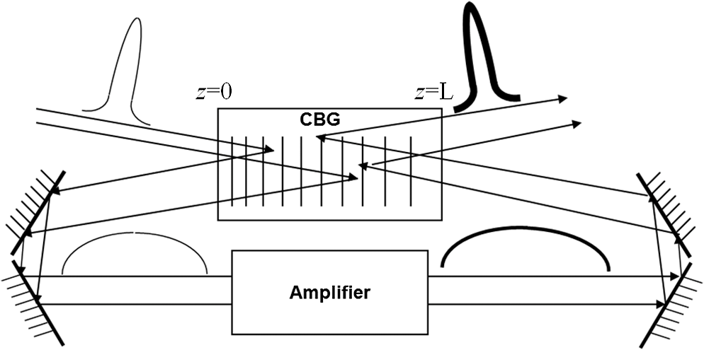
1.

Introduction

Chirped pulse amplification¹ is the main approach for high-power/high-energy ultrashort laser pulse’ generation. It is achieved by stretching ultrashort laser pulses. Those stretched pulses have a much lower value of instantaneous power and, therefore may be amplified by broadband laser amplifiers without damaging the medium. Amplified chirped pulses may then be directed to the compressing element, which allows collection of all spectral components back into ultrashort pulse, but with higher energy. The conventional way for doing this is the use of a pair of diffracting gratings for both stretching and compression (Treacy stretchers and compressors¹). An especially elegant idea was suggested and implemented by Galvanauskas et al.^2,3 with the use of chirped fiber Bragg gratings, which are gratings with a gradually varied period along the fiber. It is possible to use the same grating for compression, and stretching stage, but to illuminate it from the opposite end. In this case, the influence of smooth heterogeneities of time-delay dispersion (TDD) at the stretching stage, $T_{\mathrm{str}}(\lambda )$, is compensated for by those of the compression stage, so that $T_{\mathrm{str}}(\lambda )+T_{\mathrm{compr}}(\lambda )\approx \mathrm{const}$. A similar performance was demonstrated with the use of chirped volume Bragg gratings (chirped VBGs or CBGs), which are produced by holographic recording in the bulk of photo-thermo-refractive (PTR) glass and have dramatically higher apertures when compared with those of fiber gratings.⁴ Recent development of VBGs based on PTR glass⁵ allowed for operation of stretching-compression schemes at much higher values of power, see for example, Ref. 6.

The present paper is devoted to the development of numerical and analytic tools for the study of stretching and compression by volume CBGs. While this analysis is applicable for any volume CBG, the examples shown in this paper are based on CBGs recorded in PTR glass.

2.

Basic Scheme and System of Equations, Definition of Chirp, and Time-Delay Dispersion

The basic scheme of stretching, amplification of stretched pulse, and subsequent recompression back into short pulse by means of a volume CBG is presented in Fig. 1. Due to gradual variation of CBG period in the $z$ direction, different spectral components of an incident pulse are reflected from different parts of the CBG and, therefore, have different delays. After amplification, the stretched pulse is launched to the same CBG from the opposite side and compressed back to its original width. In this work, we consider the amplifier as a linear device that does not affect any parameters of a laser pulse but power. Therefore, we assume that a CBG-reflected stretched pulse is transmitted from the cross-section at the front surface of the CBG ($z=0$) to the opposite end of the same CBG ($z=L$), without any additional distortions.

Fig. 1

Basic scheme of stretching–amplification–compression via Chirped Bragg grating (CBG).

We assume that the dielectric permittivity and magnetic permeability of CBG depend on coordinate $z$ as

Here, smooth heterogeneity $n_2(z)$ and spatial modulation $n_1(z)$ are small in comparison with $n_0$ and are relatively slow varying functions of $z$; $\psi (z)$ is a differentiable function, and $Q$ ($\mathrm{rad}/\mathrm{m}$) has the value close to $2k$, see Eq. (13). (It should be emphasized that our notation $n_2(z)$ for the smooth correction to the background refractive index has nothing to do with the nonlinearity of refractive index.) In the standard approach of slow varying envelope approximation (SVEA), one should ignore second derivatives of slowly varying amplitudes $A(z)$ and $B(z)$, keep the resonant terms $\propto \exp (ikz)$ and $\propto \exp (-ikz)$ only, and equalize each of them to zero. As a result, one gets the following system of coupled equations:

It is convenient now to introduce new amplitudes $a(z)$ and $b(z)$, defined by

Then for these small amplitudes $a(z)$ and $b(z)$, one gets our system in the form

Possible background absorption in the medium with coefficient $\alpha (1/m)$, for intensity $I(z)\sim \exp (-\alpha z)$, may be described by purely imaginary $n_2(z)$, namely $n_2(z)=i\lambda \alpha /4\pi$.

Solution of the linear system of ordinary differential equations [Eq. (7)] may be represented as the solution of the Cauchy problem, where both boundary values are known at the same point, e.g., at $z=0$. Linearity of the system allows writing.

The amplitude of reflection and transmission for the opposite boundary conditions may be expressed through the elements of the same matrix $\widehat{M}(L)$.

Subsequently, we neglect the $n_2(z)$ term. Then, equating the local value of detuning $\nu (z)$ to zero, one can find the position $z_B(\lambda )$ of the point of exact Bragg resonance for the given vacuum wavelength $\lambda$.

Here ${\lambda }_0$ is the central wavelength defined by basic parameter of CBG: $Q=4\pi n({\lambda }_0)/{\lambda }_0$, with $Q$ defined by Eq. (4). This condition allows connecting spectral chirp parameter $\mathrm{d}\lambda /\mathrm{d}{z}_B$ of CBG with the second derivative of the phase correction $\psi (z)$. Indeed, one has to assume $\lambda =\lambda (z)$ in Eq. (13) and take $z$-derivative of the left- and right-hand sides of that equation. As a result, one gets

Here the expression for $n_{\mathrm{gr}}$ is an alternative form of denoting group velocity, $v_{\mathrm{gr}}=\mathrm{d}\omega /\mathrm{d}k=c/n_{\mathrm{gr}}$ and $n_{\mathrm{gr}}=n(\omega )+\omega (\mathrm{d}n/\mathrm{d}\omega )\equiv n(\lambda )-\lambda (\mathrm{d}n/\mathrm{d}\lambda )$. Constant chirp ($\mathrm{d}\lambda /\mathrm{d}{z}_B=\mathrm{const}$) corresponds to $\psi (z)=\beta ·{(z-0.5L)}^2$, where the mid-point $z=0.5L$ of CBG with length $L$ has resonant wavelength ${\lambda }_0$. Indeed,

In the approximation of unchanged group velocity $v_0=c/n_{\mathrm{gr}}$, the value of time-delay in the stretching process as a function of wavelength $\lambda$ is

We will see below (Fig. 7 in Sec. 5.3) that this formula yields a reasonable result for CBG with low efficiency only.

3.

Analytic Expression of Diffraction Efficiency of CBG

Consider first a weak CBG for which the first order of perturbation theory is valid. In the zeroth approximation and at $n_2\equiv 0$, one can take $A(z)\approx 1$ for all $z$. Then for the reflection amplitude coefficient, one gets from Eq. (5)

An analytic expression has been derived in Ref. 8, which is valid for any strenth of coupling. It may be simplified for constant chirp profile of the grating, with the use of Eq. (15) to:

Derivation of this expression, see Refs. 7 and 8, is similar to the calculation of quantum-mechanical transmissivity of parabolic potential barrier, see Ref. 9, and will not be discussed here. To go over the rather heavy derivation of Eq. (19) from Refs. 8 and 7, we suggest using the known structure of Eq. (19) and checking all the coefficients in it via the first-order perturbation result [Eq. (18)]. Actual numerical modeling (see below) confirmed the validity of Eq. (19) with great accuracy, especially for apodized CBG, where spatial refractive index modulation comes smoothly to zero at the ends of CBG in this particular modeling, see Eq. (40).

4.

Approximate Expression for Time-Delay Dispersion

Approximate evaluation of TDD may be done on the basis of assumption of slowly varying behavior of the coefficients $\kappa =k(z)$ and $\nu =\nu (z)$ in Eq. (7). We take the SVEA equations in the symmetric form.

In the assumption of $\nu =\mathrm{const},\kappa =\mathrm{const}$, the solution of the form $(a,b)=\exp (pz)(a_0,b_0)$ exists. From that we get the result for two eigenvalues of matrix $\widehat{V}$.

We define the positive root as the one for which, in the region $|\kappa |<|\nu |$, the real square root $\mu =+\sqrt{{\nu }^2-{|\kappa |}^2}$ satisfies the condition $\mu /|\mu |=\nu /|\nu |$; in other words, the sign of $\mu$ is the same as the sign of $\nu$ in that region where propagation is not forbidden. Eigenvectors for $p_1=+i\mu$ and for $p_2=-i\mu$ are, respectively,

Group velocity of the wave $a$ in the absence of coupling, $|\kappa |=0$, is taken as ${\mathrm{v}}_{\mathrm{a}}={\mathrm{v}}_0$, while group velocity of the wave $b$ is taken as ${\mathrm{v}}_{\mathrm{b}}=-{\mathrm{v}}_0$. The general expression for the group velocity in the presence of both constant values $\nu$ and $\kappa$ for a given mode may be intuitively written as

In the approximation of constant (or reasonably slow varying) $\nu$ and $\kappa$, one gets for mode #1 (a predominantly $a$-wave) and for mode #2 (a predominantly $b$-wave)

We take those expressions as approximations for group velocities of incident and reflected waves in the use of CBG for the stretcher-compressor scheme and verify the degree of their validity by comparison with results of direct wave modeling of CBG, Sec. 5.

In this approximate approach (Fig. 2), the incident wave $a$ (the one to be stretched by CBG) propagates from the point $z=z_1$ of the left boundary of CBG to the left point $z=z_2$ inside CBG, where decisive reflective transformation of $a$ into $b$ takes place. The points $z=z_2$ and $z=z_3$ are defined by the condition $\nu (z_{2,3},\lambda )=\pm |\kappa |$. In CBG approximated by constant chirp, $\nu (z,\lambda )=\beta ·[z-z_{\mathrm{B}}(\lambda )]$, those points are symmetrically positioned around $z_{\mathrm{B}}(\lambda )$, i.e., around perfect Bragg-resonant point.

Fig. 2

Transmitting and reflecting wave propagation in CBG. Here $L$ is the total thickness of CBG; $z=z_2$ is the point where the input wave $a$ of the given frequency $\omega =2\pi c/\lambda$. hits the region forbidden for propagation (marked by curved dashed line).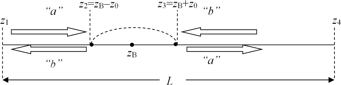

After the decisive reflection from the point $z=z_2$, incident wave of type $a$ gets transformed into reflected wave of type $b$. Total time-delay due to propagation from the entrance $z=z_1$ to reflection point $z=z_2$ and back is

Equation (15) yields the expression for $d\lambda /dz$. Here ${\lambda }_0$ is the central wavelength of CBG. In that case, $z_2=z_{\mathrm{B}}(\lambda )-z_0,z_3=z_{\mathrm{B}}(\lambda )+z_0,z_0=|\kappa |/\beta$, and integrals may be found analytically.

In the case when both $z_0\ll z_{\mathrm{B}}(\lambda )$ and $z_0\ll L-z_{\mathrm{B}}(\lambda )$, one can expand $T_{\text{cycle}}(\lambda )$ in terms of small ratio $z_0/L$.

One should take the value of $T_{\text{cycle}}$ from Eqs. (31) or (32) above and then average the expression over the spectral content of the pulse in question. As an even more crude estimate, one may try to take the value of $T_{\text{cycle}}$ at $|z_{\mathrm{B}}-L/2|\ll z$, and then the formula for time-delay of the peak of recompressed pulse becomes

It is worth discussing separately two effects that influence the delay time of the cycle stretching–recompression.

The first one is that the round-trip length of the stretching process is shorter than $2[z_{\mathrm{B}}(\lambda )-z_1]$ by the thickness of forbidden zone: $2z_0=2|\kappa /\beta |$, see Fig. 2. This leads to a shorter delay time of the stretching–recompression cycle: shorter by approximately $(4z_0/{\mathrm{v}}_0)$, i.e., of the first order in $z_0$.

The second effect is due to considerable ($\sim 50\%$ and more) decrease of group velocities in the vicinity of reflection points $z=z_2$ and $z=z_3$. The thickness of this vicinity is of the order of $z_0$. Thus, this second effect results in a longer delay time, also of the first order in $z_0$.

What is truly remarkable is that these two effects compensate each other in the first order in $z_0$. The resulting delay time does decrease (in comparison with $2L/{\mathrm{v}}_0$), but in the second order in the coupling constant, i.e., proportionally to $z_0^2$.

A monochromatic wave stretches in time from $t=-\infty$ to $t=+\infty$. One can define time delay dispersion $\mathrm{TDD}(\lambda )$ for the quasi-monochromatic packet with the wavelength $\lambda$. Many sources advise to one calculate the phase of reflection coefficient $\phi (\lambda )=\arg (r(\lambda ))$ and postulate that

Our numeric modeling shows that this is valid for large modulation of $\phi (\lambda )$ only, $|\phi |\gg 1$.

5.

Numerical Modeling

5.2.

Modeling of Stretching–Compressing by CBG with Imperfections

It should be noted that CBGs with large apertures and long stretching times^4,6,11 show some spatial variations of phase resulting from optical aberrations in a holographic recording system and optical homogeneity of a recording material (PTR glass). This is why, among other results of our numerical modeling of stretching–compression process, we would like to discuss here the influence of small and very inhomogeneous variations of phase of the grating. Equation (13) allows finding the position $z_{\mathrm{B}}(\lambda )$, where formal Bragg condition is satisfied for a given wavelength $\lambda$. We took a small oscillatory addition to the phase, $\delta \psi =a\cos \gamma z$, where $\gamma [1/\text{meter}]=2\pi /{\mathrm{\Lambda }}_1$ and ${\mathrm{\Lambda }}_1$ is the period of perturbations. Since the term $d\psi /dz$ is present in the right-hand side of Eq. (13), the equation for detuning $z_{\mathrm{B}}(\lambda )$ becomes

Eq. (37)

$$\frac{2\pi n(\lambda )}{\lambda }=\frac{2\pi n({\lambda }_0)}{{\lambda }_0}-\beta (z_{\mathrm{B}}-b)+a\gamma \sin \gamma z_{\mathrm{B}}.$$

If $a{\gamma }^2$ is larger than $2|\beta |$, then there is a possibility that Eq. (37) has several solutions ${(z_B)}_1$,${(z_B)}_2$, … for the given wavelength $\lambda$. Then application of the simplest formula

Eq. (38)

$$\mathrm{TDD}(\lambda )\approx 2(z_{\mathrm{B}}(\lambda )-z_1)/{\mathrm{v}}_0,$$

yields multivalued $\mathrm{TDD}(\lambda )$ and gives a suspicion of low-quality recompression, to say nothing about peculiar oscillations, which are even more severe in the stretched pulse. However, the results of our numerical modeling show for phase modulation

Eq. (39)

$$\delta \psi =a\cos (\gamma z)·\exp (-{(z-0.5L)}^2/d^2),d=L/4$$

that if the amplitude $2a$ (top to bottom) is moderately small, e.g., $2a\le 0.4\mathrm{rad}$, the influence of formally multivalued feature of $\mathrm{TDD}(\lambda )$ from Eq. (38) is not important. In particular, Fig. 3 shows z-dependence of Bragg resonant wavelength detuning (in nanometers) for particular perturbation of the phase given by Eq. (39). Actual wave modeling of stretching by perturbed CBG was done for $L=0.1\mathrm{m}$ and $\beta =8·{10}^4\mathrm{rad}/{\mathrm{m}}^2$, coupling coefficient $|\kappa |=S/L$, and $S=30$. Additional modulation $\delta \psi$ from Eq. (39) was taken with the parameters $2a=0.4\mathrm{rad}$, $\gamma =1405\mathrm{rad}/\mathrm{m}$. so that $a{\gamma }^2/2\beta =2.47$, and the condition of multivalued function $\mathrm{TDD}(\lambda )$ from Eq. (38) was satisfied. Stretching and compression of incident Gaussian pulse with ${\tau }_0(\mathrm{HW}{e}^{-2}\mathrm{IM})=3.0\mathrm{ps}$ was modeled and depicted in Fig. 4. It shows spectra of the incident pulse (upper curve) and of the recompressed pulse (lower curve). One can see that for a CBG with spectral width $\mathrm{\Delta }\lambda (\mathrm{FW})\approx 0.1\mathrm{nm}$ equal to that of a laser pulse at the level of $1/e^2$, the spectral width of a recompressed pulse is practically the same. However, there is some modulation of the spectrum in the vicinity of the maximum, which is caused by ripples in the dispersion curve depicted in Fig. 3; cutting off short- and long-wavelength wings of the spectrum and the spectral width of the CBG is due to finite spectral width of CBG.

Fig. 3

Dependence of Bragg resonant wavelength detuning on position inside CBG. Particular perturbation of the phase is given by Eq. (39) with top-to-bottom modulation $2a=0.4\mathrm{rad}$. Given wavelength corresponds to one or three resonant points.

Fig. 4

Spectra of Fourier transform–limited incident pulse (upper curve) and of recompressed pulse (lower curve); time duration of input pulse $\mathrm{\Delta }t$ $({\mathrm{HWe}}^{-2}\mathrm{IM})=3\mathrm{ps}$.

Figure 5 shows the intensity profiles of the input pulse, stretched pulse (multiplied by factor 80 for illustrative purposes), and recompressed pulse for CBG with the above oscillatory perturbations of the phase $\delta \psi (z)$ of the grating. Input pulse was a transform-limited Gaussian pulse with $\mathrm{\Delta }t(\mathrm{HW}{e}^{-2}\mathrm{IM})=3\mathrm{ps}$. The properties of CBG are the same as for Figs. 3 and 4. There is a small precursor in the recompressed pulse (arrow in Fig. 5) containing ~6% of recompressed energy. Nevertheless one observes rather good quality of recompression: diffraction efficiency of full cycle of stretching–compression for energy was 0.92 and ratio of peak intensities was 0.61. It means that steep perturbation of phase $\delta \psi$ with amplitude $2a\lesssim 0.4\mathrm{rad}$ is not harmful for recompression. Meanwhile, our modeling for perturbations with amplitude $2a\gtrsim 0.4\mathrm{rad}$ had shown considerable hindering recompression.

Fig. 5

Intensity profiles of input pulse (left), stretched pulse (multiplied by factor 80 for illustrative purposes, center), and recompressed pulse (right) for CBG with oscillatory perturbations of phase $\delta \psi (z)$ of the grating. Arrow points to a precursor in the recompressed pulse containing $\sim 6\%$ of its energy.

5.3.

Study of Time-Delay Dispersion

For the evaluation of our analytic (but approximate) results for time-delay dispersion, TDD($\lambda$), we had to choose a special approach in numerical modeling. Namely, illumination of CBG by a very short incident pulse ($<1\mathrm{ps}$ and therefore with a very broad spectrum) resulted in a stretched pulse with very flat top, for which it was difficult to find TDD at the stretching stage. If any distortions in the temporal profile of stretched pulse were present, the arrival time of the peak of reflected pulse was difficult to determine. On the other hand, if the incident pulse was relatively long (and hence was relatively narrow-band), the reflected pulse was not stretched to full possible duration $2L/{\mathrm{v}}_{\mathrm{gr}}$. Here ${\mathrm{v}}_{\mathrm{gr}}$ is the group velocity at ${\lambda }_0$ in unexposed glass. Still, determining the delay time for stretching stage was difficult due to large duration of the input pulse.

For that reason we calculated from numerical wave modeling the delay time of a recompressed pulse in comparison with the arrival time of an incident pulse. The delivery of the stretched pulse to the back of CBG for recompression was considered to be instantaneous in the modeling. Two types of CBG were considered. One type was with $|\kappa |=S/L$ taken as a constant through the whole thickness $L$ of CBG; hereafter, we call this type of CBG as uniform or nonapodized. The other type had the profile

Eq. (40)

$$|\kappa (z)|=\frac{S}{L}·\mathrm{apod}(z);\mathrm{apod}(z)=1-{(\frac{2z}{L}-1)}^{10}.$$

This apodization function suppressed not-quite Bragg contributions of the ends of CBG; the latter contribution leads to Fresnel function-like oscillations in the reflection spectrum of nonapodized CBG. For both cases we calculated TDD (at ${\lambda }_0=1.06\mu \text{m}$) for different values of dimensionless parameter $S$ (and for constant chirp $\beta =8·{10}^4\mathrm{rad}/{\mathrm{m}}^2$). The results for TDD slightly varied as a function of duration of input Gaussian pulse ${\tau }_0$ ($\mathrm{HW}{e}^{-2}\mathrm{IM}$). The shortest pulse duration ${\tau }_0$, for which this CBG still reflected almost all the spectrum, was ${\tau }_0=3.0\mathrm{ps}$. The stretched pulse in both cases had a duration of $\sim 1\mathrm{ns}$, i.e., 300 times longer than the input one.

Figure 6 shows the comparison of numerical modeling of time-delay $T_{\text{cycle}}$ with our analytic approximation, Eqs. (27), (28), and (33). The square points in Fig. 6 show full duration of stretching–recompression process versus dimensionless coupling coefficient $S=|\kappa |L$ for unapodized CBG. Triangular points describe corresponding data for apodized CBG. Dashed and dotted lines are calculated by the analytic model [Eqs. (27) and (28)]. Parabolic curve describing the simple formula [Eq. (33)] (not shown) is almost the same as the dashed curve for unapodized CBG. We see quadratic deviation of those curves from $2L/{\mathrm{v}}_0$ (form horizontal line) versus coupling $|\kappa |=S/L$. All data are for the input pulses with ${\tau }_0=12.0\mathrm{ps}$ at the central wavelength ${\lambda }_0=1.06\mu \text{m}$ of our CBG. We see that the approach used in the derivation of the integrals [Eqs. (27), (28), and (33)] yields very reasonable correspondence with the results of numerical modeling.

Fig. 6

Dependence of total time-delay between incident short pulse [Gaussian, with $\mathrm{\Delta }t$ [$({\mathrm{HWe}}^{-2}\mathrm{IM})=12\mathrm{ps}$] and recompressed pulse on the dimensionless coupling coefficient $S=|\kappa |L$. Square and triangular points correspond to numerical modeling of unapodized and apodized CBG, respectively. Dashed and dotted lines for corresponding CBG yield the results calculated by analytic model Eqs. (27) and (28). Parabolic curve describing simple formula Eq. (33) (not shown) is almost the same as dashed curve for unapodized CBG. We see quadratic deviation of those curves from $2L/v_0$ (from horizontal line) versus coupling 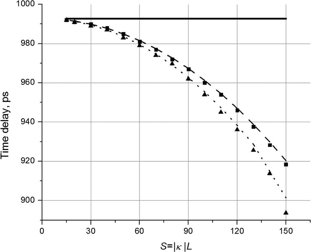$|\kappa |=S/L$.

Here is an important (and originally unexpected) observation. Too large a value of coupling ($S\ge 70$) for that particular CBG and ${\tau }_0=3.0\mathrm{ps}$, while yielding 99.4% diffraction efficiency for energy of recompressed pulse, resulted in relatively poor quality of recompression: peak intensity of recompressed pulse constituted 52% of the incident one. Our interpretation of that decrease of recompression quality is the following. Different spectral components of incident pulse exhibit somewhat different values of the sum $T_{\text{cycle}}(\lambda )=T_1(\lambda )+T_2(\lambda )$, from integrals [Eqs. (27) and (28)] with different values of $z_{\mathrm{B}}(\lambda )$, see Fig. 7 for apodized CBG with $S=90$. The presence of shorter values of $T_{\text{cycle}}(\lambda )$ points to the formation of precursor in the recompressed pulse. This effect leads to deteriorated recompression. Meanwhile, the fact that two considerably distant wavelengths have those shorter values of $T_{\text{cycle}}(\lambda )$ explains interference-type oscillations in the precursor.

Fig. 7

Dependence of stretching time $T_1(\lambda )$ calculated by Eq. (27) for apodized CBG with $S=90$, compression time $T_2(\lambda )$, Eq. (28), time of cycle stretching–compression $T_{\text{cycle}}(\lambda )=T_1(\lambda )+T_2(\lambda )$, time of double pass through blank glass $2L/{\mathrm{v}}_0$.

6.

Conclusions

We have developed a detailed Mathematica-based numerical tool for modeling the process of stretching–recompression by CBG with arbitrary profiles of the grating’s phase and coupling coefficient. To better understand the results of numerous variants of that modeling, we developed approximate analytical model of time-delay dispersion $\mathrm{TDD}(\lambda )$. An unexpected result of that analytic model is that dependence of TDD on the coupling constant $|\kappa |=S/L$ starts with terms proportional to $|\kappa {|}^2$. We have shown that excessively large coupling in CBG leads to deterioration of recompression quality. We show that perturbations of grating phase with small ($<\sim 0.4\mathrm{rad}$ top-to-bottom) amplitude do not hinder the recompression quality much, enabling $>90\%$ of energy in the recompressed pulse.