Efficient active depth sensing by laser speckle projection system

Xuanwu Yin; Guijin Wang; Chenbo Shi; Qingmin Liao

doi:10.1117/1.OE.53.1.013105

20 January 2014 Efficient active depth sensing by laser speckle projection system

Xuanwu Yin, Guijin Wang, Chenbo Shi, Qingmin Liao

Author Affiliations +

Optical Engineering, Vol. 53, Issue 1, 013105 (January 2014). https://doi.org/10.1117/1.OE.53.1.013105

Abstract

An active depth sensing approach by laser speckle projection system is proposed. After capturing the speckle pattern with an infrared digital camera, we extract the pure speckle pattern using a direct-global separation method. Then the pure speckles are represented by Census binary features. By evaluating the matching cost and uniqueness between the real-time image and the reference image, robust correspondences are selected as support points. After that, we build a disparity grid and propose a generative graphical model to compute disparities. An iterative approach is designed to propagate the messages between blocks and update the model. Finally, a dense depth map can be obtained by subpixel interpolation and transformation. The experimental evaluations demonstrate the effectiveness and efficiency of our approach.

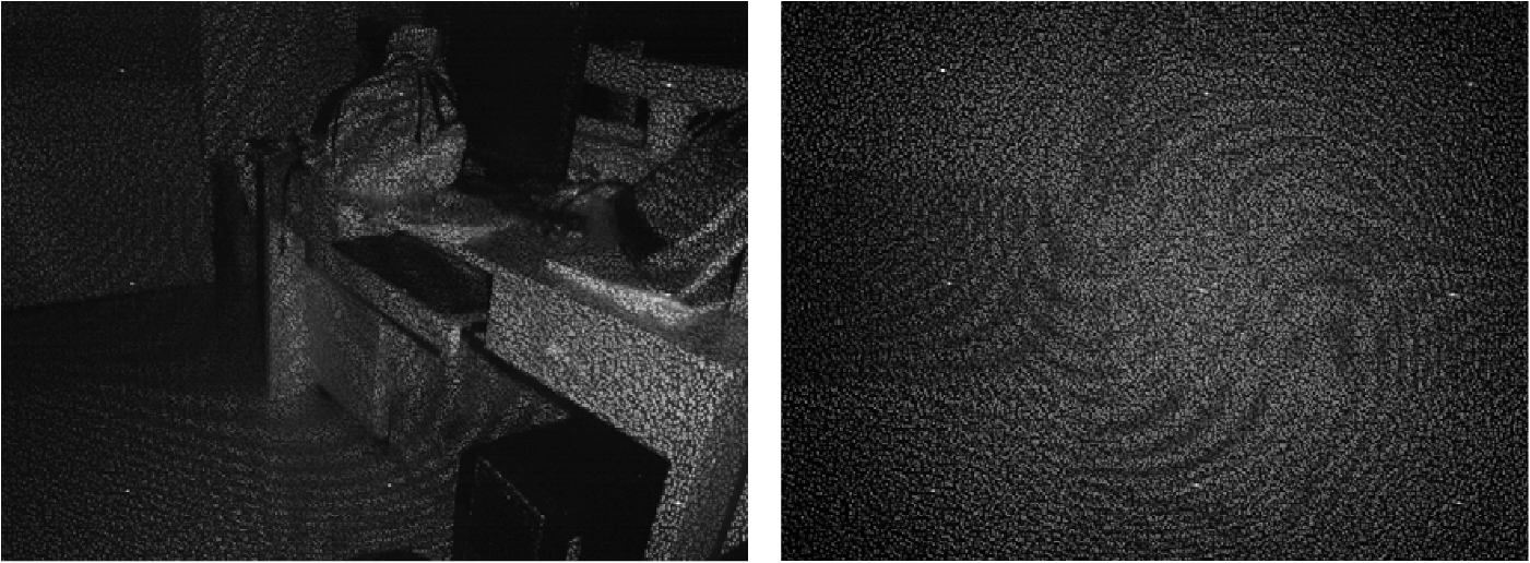
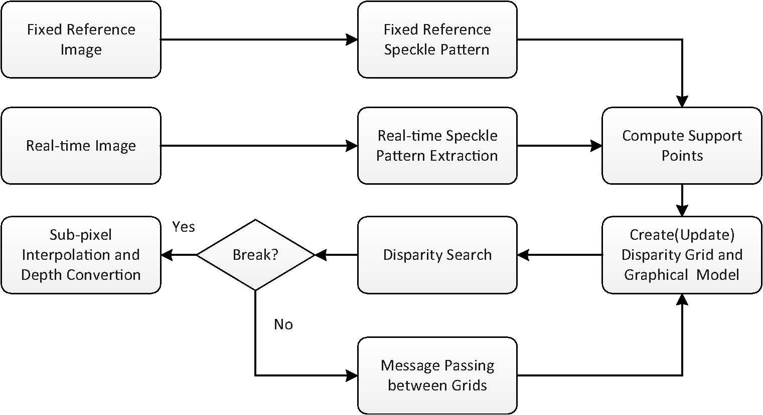
1. Introduction

Depth estimation is a basic problem in computer vision, widely applied in fields as diverse as automatic driving, shape measurement in industry, biomedical imaging, and human-computer interaction. Refer to Ref. 1 for an overview.

In recent years, estimating depth by speckle projection has attracted considerable attention. Siebert and Marshall² introduced three structures of speckle systems to capture three-dimensional (3-D) human body. Garcia et al.³ used ground glass to generate speckles and computed depth by correlating the captured image with reference images at different depth layers. Chen and Chen⁴ projected speckles with a common projector and built up a binocular system. Schaffer et al.⁵ used a laser and a diffuser to generate speckles and computed the depth using a temporal correlation method. However, these systems are restricted to near range and cannot be applied in bright environment due to the use of visual light. Recently, researchers tended to use infrared projectors and cameras⁶^,⁷ to expand the sensing range for indoor applications. In these systems, the depth was estimated by stereo matching⁸ between the real-time captured image and the reference image. However, the high contrast of speckles could not be well handled by conventional methods. Wang et al.⁹ utilized adaptive binarization to handle the high contrast and proposed a progressive approach to estimate the depth map. Nevertheless, none of the approaches mentioned has considered the impact of ambient lighting.

To tackle these problems, in this paper, we propose a novel approach to sense the indoor depth information. In our system, infrared laser speckle pattern is projected onto the scene and a single camera is used to capture images. First, we propose a novel direct-global separation approach to remove the ambient lighting and extract the pure speckle pattern. After that, a set of sparse support points are selected. Then a disparity grid is built upon these support points and a generative graphical model is introduced to search disparities. We propagate messages between blocks and update the disparities and the model iteratively. Finally, the depth map can be obtained by transforming the disparities into depth values. The experiments demonstrate the efficiency and effectiveness of our approach.

The rest of this paper is organized as follows. In Sec. 2, we present the system structure and the framework of the algorithm. The preprocessing, including speckle pattern extraction and feature computing, is introduced in Sec. 3. Section 4 presents how to build the graphical model and search for the disparities with this model. Experimental results are presented in Sec. 5. In the last section, we make a conclusion and a discussion of future work.

2. System Structure and Algorithm Framework

As shown in Fig. 1, the system is made up of one pattern projector and one infrared digital camera. We use the Kinect’s projector, which consists of an infrared laser generator and a diffuser, to project the speckle pattern onto the scene. Aligned with the projector in $Y$ and $Z$ direction, the infrared camera captures the real-time speckle pattern reflected by the scene.

Fig. 1

System setup.

Figure 2 gives an example of the inputs of our scheme, a real-time image and a fixed reference image. The reference image is a flat plane perpendicular to the optical axis, captured at a certain distance. Thus, the setup is equivalent to a binocular system. The depth can be computed by estimating disparities between the real-time image and the reference image.

Fig. 2

Input image pair. Left: real-time image. Right: reference image.

Figure 3 presents the framework of our proposed approach. First, we separate the direct component from the image to extract the pure speckle pattern. With this speckle pattern, we compute the matching costs of both left-to-right and right-to-left. Sparse support points are selected by evaluating the matching cost and left-right consistency. Then a disparity grid is built upon these support points. For each block in the disparity grid, we introduce a generative graphical model to represent the relationship between the support points and the unmatched points. Thus, disparities are computed by minimizing an energy function derived from the graphical model. The new reliably matched points are added as support points, and the graphical model is updated. Such process is repeated until convergence. Finally, the depth map is obtained by subpixel interpolation and transformation.

Fig. 3

Processing flow of the proposed approach.

3. Speckle Pattern Extraction and Feature Computing

As the illumination of real-time captured image and the reference image can be significantly different, it is not reliable to simply utilize local intensities¹⁰ to describe the speckles. To better describe the speckles, we first extract the pure speckle pattern, which is represented by binary features. Note that the fixed reference image is processed only once.

In the image, the intensity at $(u, v)$ , $i (u, v)$ can be viewed as a combination of two components, namely direct and global,¹¹

Eq. (1)

i (u, v) = i_{d} (u, v) + i_{g} (u, v),

where

i_{d} (u, v)

is the direct component due to direct illumination for the speckle pattern, and

i_{g} (u, v)

is the global component due to ambient lighting. Nayar et al.¹¹ used high-frequency illumination to separate the direct and global components with multiple images.

In this work, we try to extract the direct component with a single image and obtain the pure speckle pattern. By analyzing tens of images captured under various illuminations, we find that the intensities of speckles are spatially nonuniform, while the smallest values in the neighborhood of a certain radius $δ_{s}$ around the speckles are stationary. According to Ref. 12, the radius $δ_{s}$ can be fixed as constant. Figure 4 presents a representative image patch. The red inset contains a single speckle of relatively low intensity and the green inset contains four visibly brighter speckles. It can be observed that the smallest value in the red inset is almost the same as that in the green inset. That is, in a window larger than $(2 δ_{s}) \times (2 δ_{s})$ , the lowest intensities reflect the global component.

Fig. 4

A sample of real-time image and local details at different locations. (a) Sample patch in real-time image. (b) Detail for red inset in (a). (c) Detail for green inset in (a).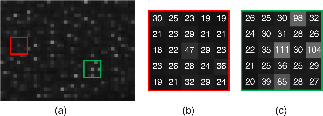

Let $x_{n}$ , $n = 1, \dots, N, \neq$ be the observed intensity values in a window of size $W_{s} \times W_{s} (W_{s} > 2 δ_{s})$ , and $X_{i}$ , $i = 1, \dots, N$ be its order statistics. The global component is estimated with the weighted average of these observations,

Eq. (2)

{\hat{i}}_{g} (u, v) = \frac{\sum_{k = 1}^{N} w_{k} X_{k}}{\sum_{k = 1}^{N} w_{k}},

with the weight defined as

Eq. (3)

w_{k} = \frac{2}{1 + \exp [λ {(X_{k} - X_{1})}^{2}]} .

The parameter $λ$ is a constant that controls the weight of each point, i.e., the contribution of a point to the estimated global component. Thus, the direct component at $(u, v)$ can be estimated by

Eq. (4)

{\hat{i}}_{d} (u, v) = i (u, v) - {\hat{i}}_{g} (u, v) .

The direct component, as the pure speckle pattern, is then utilized to compute the feature vector for each point.

To describe a certain point, we apply the CENSUS transform¹³ in a $W_{f} \times W_{f}$ window around it to form a binary feature vector, denoted as $f$ . Let $x_{n}^{d}$ , $n = 1, \dots, N$ , be the estimated direct component with Eq. (4) in this window. The feature vector $f$ can be treated as a binary string formed by a sequence of one-bit digits,

Eq. (5)

f = \sum_{i \neq N / 2} 2^{i} U (x_{i} - x_{N / 2}),

where

x_{N / 2}

is the center of the window, and

U (•)

is a step function,

Eq. (6)

U (x) = {\begin{matrix} 1 & if x \geq 0 \\ 0 & otherwise \end{matrix} .

4. Depth Estimation with Iteratively Updated Graphical Model

Once the features have been computed, we can compute correspondences between the real-time image and the reference image to estimate the disparities. Geiger et al.¹⁴ built a prior on the disparities by forming a triangulation on support points, which has been proved to be very effective. However, as there are out-of-range regions and non-Lambertian surfaces in the infrared images, the support points will not distribute as uniformly as that in their visual-light images. To cope with this problem, we built a disparity grid and introduced an iterative updating scheme inspired by Shi et al.¹⁵ and Wang et al.⁹

4.1.

Support Points

Support points are the points that can be robustly matched between the input image pair.¹⁶^,¹⁷ In this work, we select support points by evaluating the matching cost and uniqueness.

Let $o = {(u, v, f)}^{T}$ be an observation in the real-time image, defined as the concatenation of its image coordinates, $(u, v) \in N^{2}$ , and a feature vector, $f \in R^{Q}$ . Let $O^{r} = {o_{1}^{r}, \dots o_{N}^{r}}$ be the set of observations in the reference image that lie on the epipolar line associated with $o$ , with each observation formed as $o_{n}^{r} = {(u - d_{n}, v, f_{n}^{r})}^{T}$ , in which $d_{n}$ is the disparity between $o$ and $o_{n}^{r}$ . The matching cost between $o$ and $o_{n}^{r}$ is measured by the distance of the feature vectors,

Eq. (7)

Cost (o, o_{n}^{r}) = D_{f} (f, f_{n}^{r}),

where

D_{f} (•, •)

is a distance function. In this paper, Hamming distance is used. To get rid of ambiguous matches, only the points whose absolute difference between the best and second best matches is large enough are retained. The uniqueness is measured by the left-right consistency, i.e., correspondences are retained only if they can be matched from left-to-right and from right-to-left.⁹^,¹⁴

4.2.

Disparity Grid and Generative Graphical Model

To merge the local information of the support points, we build a disparity grid on the real-time image by dividing the image into $M_{g} \times N_{g}$ blocks, with each block of size $W_{g} \times W_{g}$ . The grid structure is illustrated in Fig. 5(a). For each block, the disparities of support points inside it and those in its four-neighborhood blocks are taken as the candidate disparities for it. These disparities form a candidate disparity set $D = {d c_{1}, \dots, d c_{M}}$ , $d c_{m} \in N$ . This cross-block supporting scheme allows for the effective propagation of neighboring information between blocks.

Fig. 5

Disparity grid and graphical model. (a) Grid setup and cross-block supporting. (b) Graphical model. Observations and candidate disparities are conditionally independent given $d_{m}$ , the disparity between $o$ and $o_{m}^{r}$ . And observations in $O^{r}$ are conditionally independent given 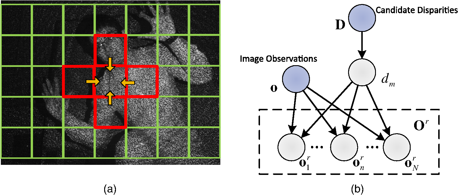$d_{m}$ and $o$ .

We propose a generative graphical model to model the relationship between the candidate disparities and the observations, and the relationship between observations, as shown in Fig. 5(b). Denote by $o$ the point we want to compute. These two relationships are described by two conditional independence assumptions:

1. the observations ${o, O^{r}}$ and the candidate disparities $D$ are conditionally independent given disparity $d_{m}$ ;
2. the observations in $O^{r}$ are conditionally independent with each other given $d_{m}$ and $o$ .

By the first assumption, the joint probability is factorized as

Eq. (8)

p (d_{m}, o, o_{n}^{r}, D) = p (o_{n}^{r} | o, d_{m}, D) p (d_{m} | o, D) p (o, D) \propto p (o_{n}^{r} | o, d_{m}) p (d_{m} | D) / Z,

with

p (o_{n}^{r} | o, d_{m})

being the likelihood,

p (d_{m} | D)

being the prior, and

Z

being the normalization factor. The prior can be modeled as an equally weighted Gaussian mixture model

Eq. (9)

p (d_{m} | D) \propto \sum_{d c \in D} \exp [- \frac{{(d_{m} - d c)}^{2}}{2 σ^{2}}] .

A constrained Laplace distribution is applied to represent the likelihood:

Eq. (10)

p (o_{n}^{r} | o, d_{m}) \propto {\begin{matrix} \exp [- β \cdot D_{f} (f, f_{n}^{r})] & if d_{m} = d_{n} \\ ϵ & otherwise \end{matrix},

where

ϵ

is a positive number, with a typical value

1.0 e^{- 6}

. The condition

d_{m} = d_{n}

is derived from the fact that given a disparity, there is a deterministic mapping of

o

in the reference image.

Once the prior and likelihood are formulated, the disparity can be estimated by the maximum a posteriori estimation,

Eq. (11)

\hat{d} = \underset{d_{m}}{argmax} p (d_{m} | o, O^{r}, D),

where

O^{r}

is the set of observations in the reference image that lie on the epipolar line associated with

o

. Similar to Eq. (8), the posterior is factorized as

Eq. (12)

p (d_{m} | o, O^{r}, D) \propto p (d_{m}, o, O^{r}, D) \propto p (O^{r} | o, d_{m}) p (d_{m} | D) .

By the second independence assumption, the conditional distribution over $O^{r}$ can be further factorized as

Eq. (13)

p (O^{r} | o, d_{m}) = \prod_{n = 1}^{N} p (o_{n}^{r} | o, d_{m}),

i.e., the product of all likelihoods. Note that the factorization in Eq. (13) holds and makes sense only if none of the likelihood takes on the zero value, which is the reason that

ϵ

is set to nonzero in Eq. (10). By plugging Eqs. (9), (10) and (13) into Eq. (12) and taking the negative logarithm, an energy function can be derived as follows:

Eq. (14)

E (d) = β \cdot D_{f} [f, f^{r} (d)] - \log {\sum_{d c \in D} \exp [- \frac{{(d - d c)}^{2}}{2 σ^{2}}]} + \log Z + C,

with

f^{r} (d)

being the feature vector at

(u - d, v)

in the reference image, and

C

being a constant associated with

ϵ

only. Now, the disparity for each point can be estimated by minimizing the energy function

Eq. (15)

\hat{d} = \underset{d}{argmin} E (d) .

4.3.

Iterative Model Updating

For out-of-range regions and non-Lambertian surfaces, the support points may not be sufficient. The disparity grid may not provide enough disparity information in these regions. To efficiently propagate the information between blocks, we propose an iterative scheme to update the support point set $D$ and the graphical model.

The key of this iterative updating scheme is to select new reliably matched points during iterations. The energy in Eq. (14) itself is powerful to measure the reliability. Suppose for $o$ , the estimated disparity is $\hat{d}$ . According to Eq. (14), the minimum matching energy is $E (\hat{d})$ . The lower $E (\hat{d})$ is, the more reliably $o$ is matched.

We also use the confidence¹⁰^,¹⁸ to describe the goodness of matching, which is defined as

Eq. (16)

Conf (\hat{d}) = \min_{\tilde{d} \neq \hat{d}} [E (\tilde{d}) - E (\hat{d})] .

This definition indicates the difference between the minimum energy and the second-minimum one.

Using both the matching energy and the confidence, we propose the iterative scheme presented in Algorithm 1 to update the model and search for $d^{*}$ , the optimal disparity for $o$ . At the beginning of each iteration, the matching energy and confidence for the points is computed with the current model. If the matching energy is lower than the current lowest matching energy $E (d^{*})$ , and the confidence is above some threshold ${TH}_{Conf}$ , $d^{*}$ will be updated to $\hat{d}$ . Furthermore, if the matching energy is lower than some threshold ${TH}_{E}$ , this point is treated as reliably matched and $\hat{d}$ will be added into $D$ . At the end of each iteration, the model is recomputed with the updated support point set $D$ .

Algorithm 1

Iterative model updating and optimal disparity searching.

1: repeat

2: for each $o$ that has not been reliably matched do

3: compute

E (\hat{d})

and

Conf (\hat{d})

with the current model

4: if $E (\hat{d}) < E (d^{*})$ and $Conf (\hat{d}) > {TH}_{Conf}$ then

5: set

d^{*} = \hat{d}

6: if $E (\hat{d}) < {TH}_{E}$ then

7: add

\hat{d}

into

D

8: end if

9: end if

10: end for

11: recomputed the graphical model with the updated

D

12: until after N iterations

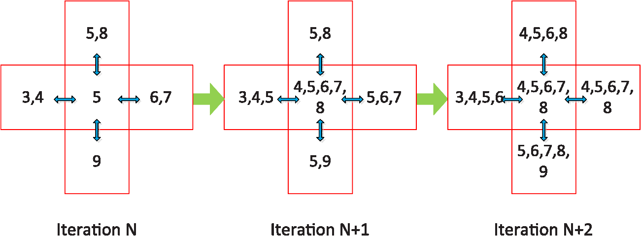
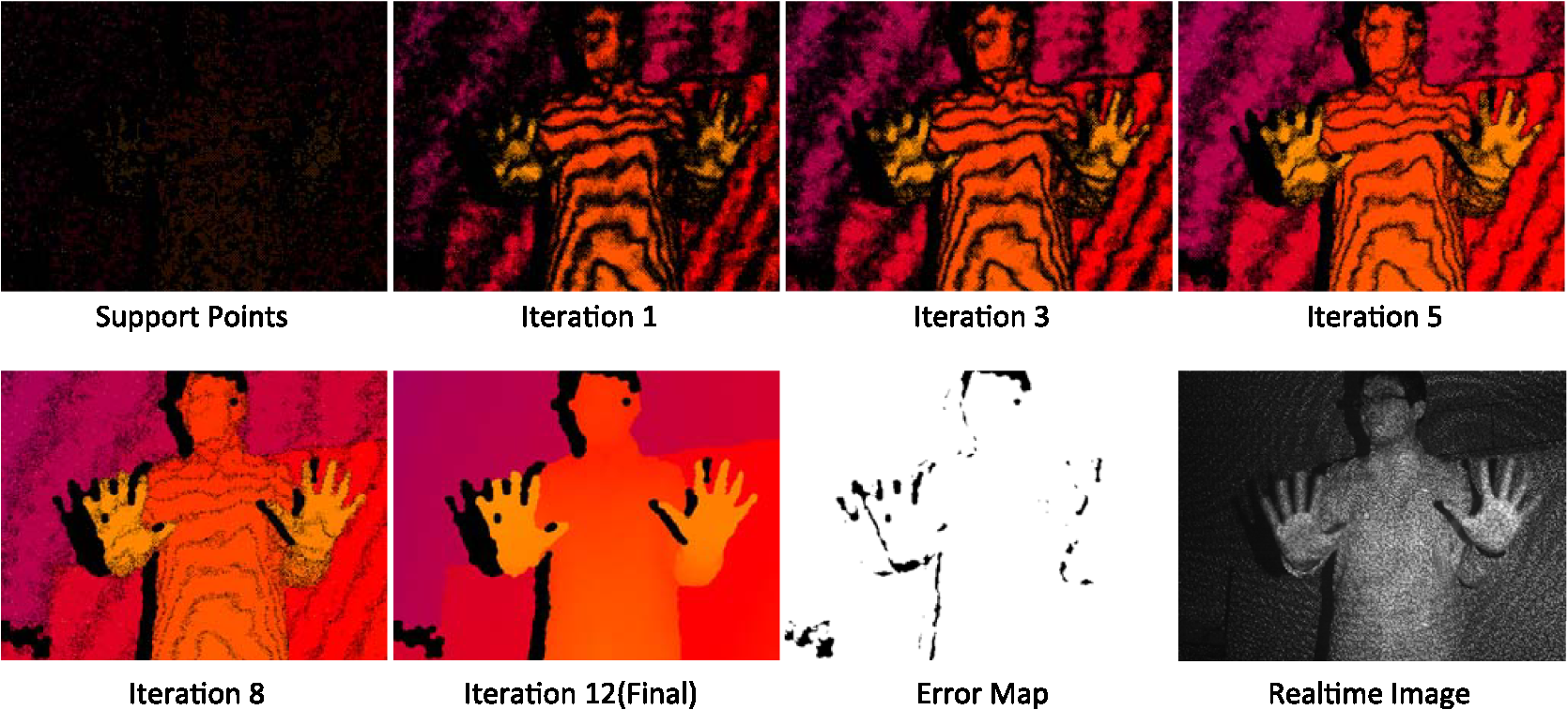
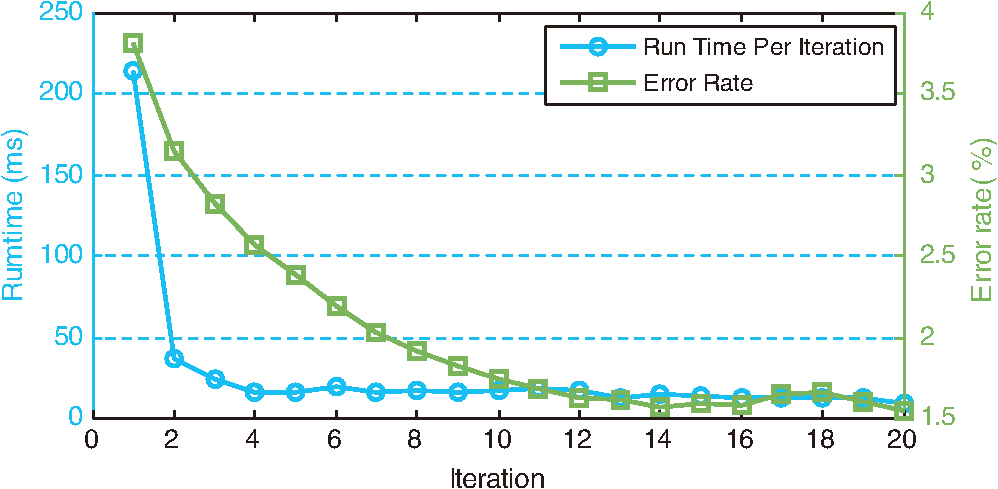
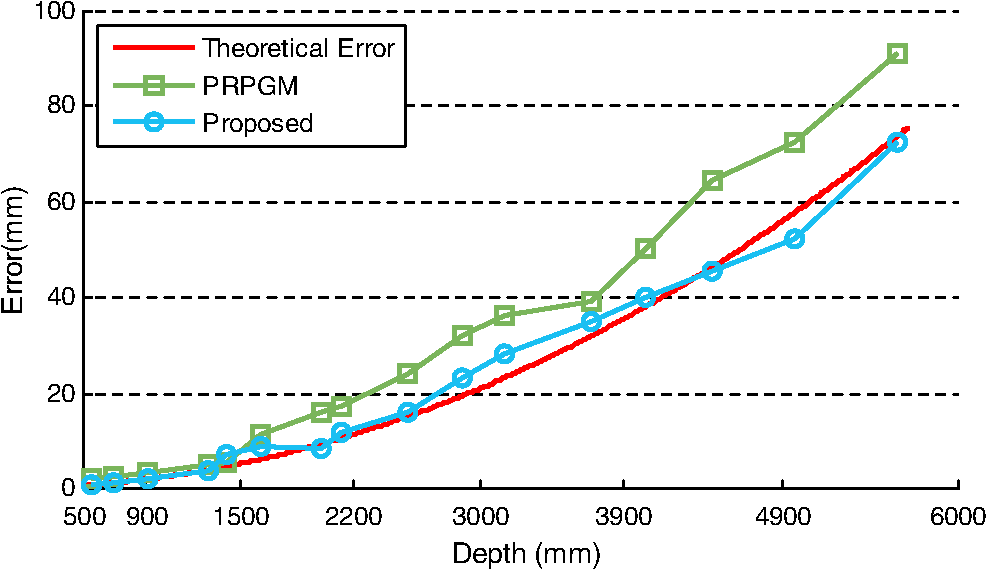
We note that because the blocks can support neighboring blocks, the newly added support points can be used to update not only the block they belong to but also the neighboring blocks. Thus, the messages can propagate between blocks during iterations. Meanwhile, the thresholds, ${TH}_{Conf}$ and ${TH}_{E}$ , can prevent the spurious messages from spreading out. Figure 6 gives an example of disparity messages propagating between blocks.

Fig. 6

Iterative message propagation. Numbers in the block are the estimated disparities of points in this block.

4.4.

Subpixel Interpolation and Depth Transformation

Interpolation has been adopted to achieve subpixel accuracy.¹⁹ We choose the linear interpolation method for its efficiency and effectiveness.

Suppose the integer disparity for a point is $d$ , and the corresponding matching energy is $E (d)$ . Let $Δ L = | E (d) - E (d - 1) |$ and $Δ R = | E (d) - E (d + 1) |$ , the subpixel disparity $d_{sub}$ is computed by

Eq. (17)

d_{sub} = {\begin{matrix} d + (Δ L / Δ R - 1) / 2, & if Δ L \leq Δ R \\ d - (Δ R / Δ L - 1) / 2, & if Δ L > Δ R \end{matrix} .

According to the triangular geometry, we can derive depth $Z$ from disparity $d_{sub}$ as

Eq. (18)

Z = \frac{s}{d_{sub} + s / Z_{0}},

where

s

is a constant determined by the focal length of the camera and the equivalent baseline length, and

Z_{0}

is the depth of the reference plane.

5. Experimental Evaluation

To evaluate the performance, we implement our approach in C++ on a desktop computer with 2.50 GHz Q9300 CPU and 4GB RAM. First, the effectiveness of pattern extraction and binary feature is presented. Then we show the efficiency and accuracy of the algorithm. Last, we give more results of several different scenes and compare our approach with other methods. Throughout all experiments, the parameters are fixed as $W_{s} = 5$ , $λ = 0.05$ , $W_{f} = 15$ , $σ = 0.5$ , $β = 0.05$ , ${TH}_{E} = 100$ , ${TH}_{Conf} = 24$ .

5.1.

Speckle Pattern Extraction and Binary Feature

As shown in Fig. 7, except for defocus blurred and saturated regions, most of the direct components can be extracted clearly. To show the effectiveness of our speckle pattern extraction method and binary feature, we test the algorithm on a typical scene that contains surfaces of different depths. We run the algorithm with or without the speckle pattern extraction using the binary or intensity feature, four combinations in total. The comparison is presented in Fig. 8.

Fig. 7

Speckle pattern extraction result. (a) Original real-time image. (b) Global component (ambient lighting). (c) Direct component (speckle pattern). The green inset indicates a defocus blurred region, the red inset indicates a saturated region, and the blue inset indicates a normal region.

Fig. 8

Effectiveness of speckle pattern extraction and binary feature. (a) Real-time image. (b) Using intensity feature without pattern extraction. (c) Using intensity feature with pattern extraction. (d) Using binary feature without pattern extraction. (e) Using binary feature with pattern extraction.

From Fig. 8, it can be observed that the result is the worst for the scheme without pattern extraction and with intensity feature, while the result is the best for our scheme with the pattern extraction and with binary feature. Especially, the result is greatly improved by our scheme in faraway regions. In these regions, the low contrast between the speckle pattern and the ambient lighting make the matches ambiguous. As the speckle pattern extraction can get rid of the ambient lighting’s influence and the binary feature is insensitive to contrast, the combination of them can significantly reduce the ambiguities. It can also be seen from the results that depth stripes are more obvious when using the intensity feature, though subpixel interpolation has been applied to all setups. This indicates that the binary feature can achieve a higher accuracy than the intensity feature.

5.2.

Efficiency Analysis

To show the efficiency of the proposed approach, we test the algorithm on a scene with one person inside. Figure 9 shows some results during iterations and the error map of the final result. It can be seen that our iterative message-passing scheme make the information propagate efficiently between blocks. The experimental results show that more reliably matched points are added earlier, which is in agreement with our analysis earlier. From the error map, we can see that the proposed approach is rather accurate except for some complex boundaries, e.g., the hands of the human.

Fig. 9

Intermediate results during iterations.

Figure 10 presents the convergence of the error rate and running time. The error rate is the percentage of bad pixels whose disparity error is over some tolerance (1 pixel in this paper). We convert depth into disparity with the inverse transform of Eq. (18) to compute error rates. It can be seen from Fig. 10 that after about 12 iterations, the error rate has converged to no more than 1.7%. The running time per iteration decreases so sharply that it almost converged to a constant after four iterations. Hence, we choose to terminate the process after 12 iterations, for the balance between accuracy and efficiency. On average, the proposed approach can process more than $3 frames / s$ with the image resolution of $640 \times 480$ .

Fig. 10

Convergence of running time and error rate.

5.3.

Plane Test and Accuracy Analysis

We test the algorithm on a series of planes to analyze the estimation accuracy. These images are captured with planes perpendicular to the optical axis of the camera at different distances. By assuming that the mean value of the depth map is an unbiased estimator for the plane, the standard deviation is used to measure the estimation error. According to the analysis in Ref. 20, the theoretical random error of depth measurement is proportional to the square distance from the sensor to the object.

We compare the error of proposed method with the progressive reliable points growing matching (PRPGM) method introduced by Wang et al.,⁹ and the results are plotted in Fig. 11. The theoretical error is computed by assuming that the disparity estimation error is 0.2 pixel. The error curve shows that the error of the proposed algorithm coincides with the theoretical error. For long-range planes, the proposed method performs better than the PRPGM method and can achieve a gain about 3 dB in the absolute error. Besides, the largest relative error of our method is still $< 1.5 %$ , which verifies that the proposed approach can achieve an acceptable accuracy for different depth layers.

Fig. 11

Plane test for error analysis. Theoretical error is computed assuming that the disparity estimation error is 0.2 pixel. Depth is showed in logarithmic coordinate.

5.4.

Scene Test

To demonstrate the wide applicability of our approach, we test our method on two videos. The first video is acquired with a fixed background and a human inside; the second is acquired with complex scenes, including different kinds of objects and non-Lambertian surfaces, such as LCD.

We compare our approach with the normalized cross correlation (NCC)-based local window matching and the PRPGM method, both introduced in Ref. 9. To make the comparison fair, we apply the same speckle pattern extraction and subpixel interpolation to all three methods. Some representative frames are presented in Fig. 12, from which we can observe the following.

Fig. 12

Depth estimation under different scenes. The proposed method is compared with the NCC window matching and PRPGM method.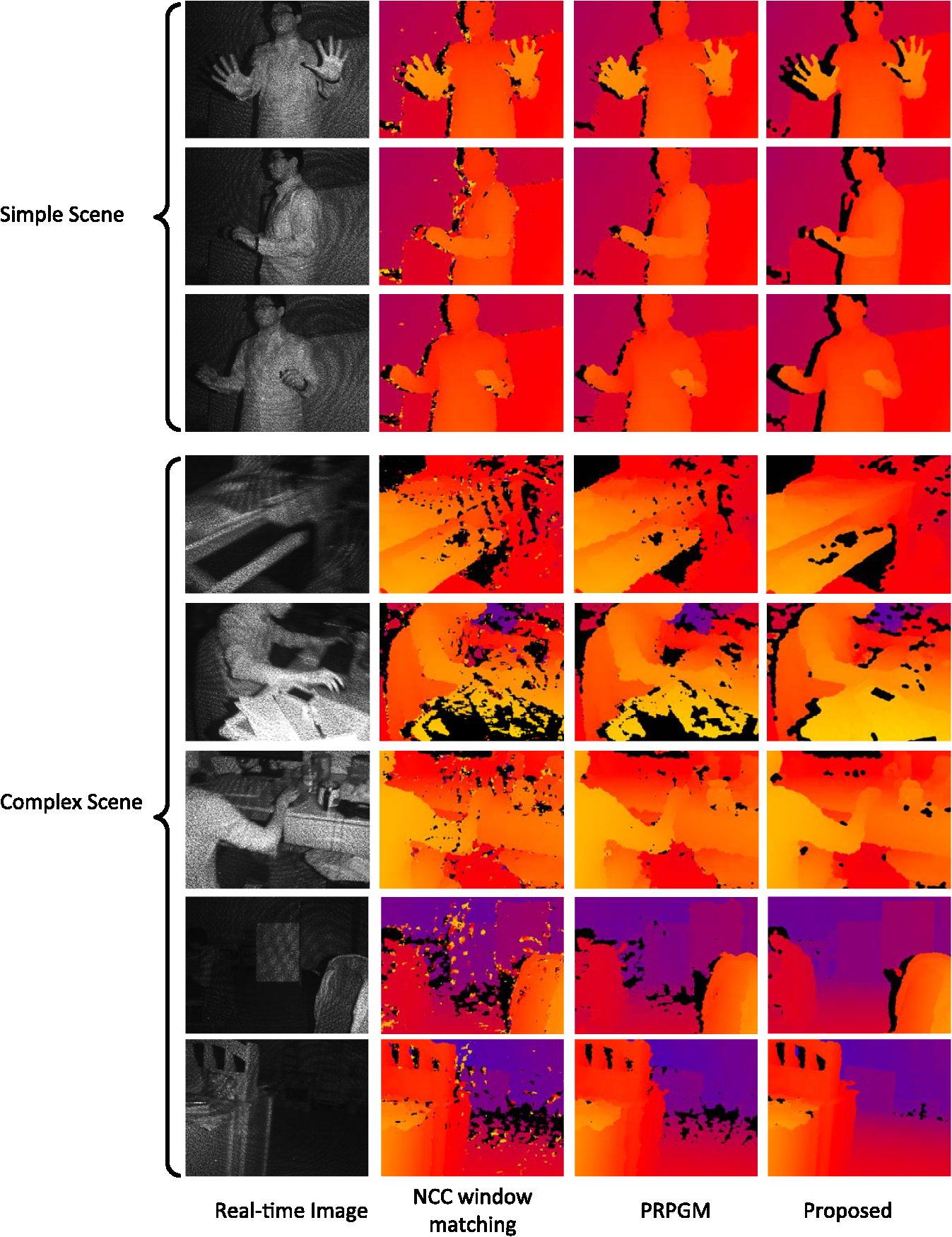

First, even though the speckle pattern extraction and the standard postprocessing are applied, there are still many mismatches left in the outcome of the NCC window matching. This indicates that the NCC method is not suitable to handle the speckle pattern, which is of high contrast.

Second, the PRPGM method behaves better than the NCC method; it has fewer holes left. This is because the reliably matched points can act as seeds to pass their disparity information to their neighbors. However, as the seeds only send out messages to their immediate neighbors, the information spreads very slowly. Points in regions of fewer seeds, such as boundaries, may receive messages from incorrect seeds. Even worse, if they are too far away from the seeds, they can hardly receive useful messages. The low speed of message passing may lead to inaccurate boundaries and unmatched patches, in particular, for complex scenes.

Third, the proposed method can cope with these problems. Through the cross-block support and the iterative model update, messages can pass on a scale of the block size. Therefore, regions with fewer support points can receive information from their neighboring blocks. Even the points in blocks of few support points can still gain substantial information after some iterations. Hence, more accurate boundaries can be obtained, and there are no unmatched patches left except for the regions where the speckle pattern cannot be extracted. The right-hand column of Fig. 12 demonstrates that our approach is widely applicable for different kinds of scenes.

Figure 13 presents the error rate of the three methods over the two videos. The proposed method can achieve the best performance for most of the cases. In the simple scenes, the proposed method can reduce about 2% of the error points compared with the PRPGM method; in complex scenes, an even greater gain can be achieved.

Fig. 13

Error rate under different scenes, compared with NCC window matching and PRPGM.

6. Conclusion and Future Work

In this paper, we have presented an active system to achieve effective depth sensing. We have shown that the speckle pattern extraction can effectively remove the ambient lighting, and the binary feature used is robust to contrast variation. The experiments have demonstrated that our iterative message-passing and model updating scheme can refine the disparity map efficiently, and our system is widely applicable. More importantly, the conditional independence in our graphical model makes it possible to process the points in parallel; thus the algorithm can be accelerated with graphics processing unit and field programmable gata array. To increase the robustness of our method, we intend to search for more robust preprocessing method, and a further plan is to refine the depth map by using the texture information of the scene.

Acknowledgments

This work is partially supported by NSFC 61271390.

References

1.

F. ChenG. M. BrownM. Song, “Overview of three-dimensional shape measurement using optical methods,” Opt. Eng., 39 (1), 10 –22 (2000). http://dx.doi.org/10.1117/1.602438 OPEGAR 0091-3286 Google Scholar

2.

J. P. SiebertS. J. Marshall, “Human body 3D imaging by speckle texture projection photogrammetry,” Sensor Rev., 20 (3), 218 –226 (2000). http://dx.doi.org/10.1108/02602280010372368 SNRVDY 0260-2288 Google Scholar

3.

J. Garciaet al., “Three-dimensional mapping and range measurement by means of projected speckle patterns,” Appl. Opt., 47 (16), 3032 –3040 (2008). http://dx.doi.org/10.1364/AO.47.003032 APOPAI 0003-6935 Google Scholar

4.

Y.-S. ChenB.-T. Chen, “Measuring of a three-dimensional surface by use of a spatial distance computation,” Appl. Opt., 42 (11), 1958 –1972 (2003). http://dx.doi.org/10.1364/AO.42.001958 APOPAI 0003-6935 Google Scholar

5.

M. Schafferet al., “High-speed three-dimensional shape measurements of objects with laser speckles and acousto-optical deflection,” Opt. Lett., 36 (16), 3097 –3099 (2011). http://dx.doi.org/10.1364/OL.36.003097 OPLEDP 0146-9592 Google Scholar

6.

FreedmanB.et al., “Depth Mapping Using Projected Patterns,” US Patent 20,100,118,123 (2010).

7.

ShpuntA.ZalevskyZ., “Depth-Varying Light Fields for Three Dimensional Sensing,” US Patent 8,374,397 (2013).

8.

D. ScharsteinR. Szeliski, “A taxonomy and evaluation of dense two-frame stereo correspondence algorithms,” Int. J. Comput. Vision, 47 (1–3), 7 –42 (2002). http://dx.doi.org/10.1023/A:1014573219977 IJCVEQ 0920-5691 Google Scholar

9.

G. Wanget al., “Depth estimation for speckle projection system using progressive reliable points growing matching,” Appl. Opt., 52 (9), 516 –524 (2013). http://dx.doi.org/10.1364/AO.52.000516 APOPAI 0003-6935 Google Scholar

10.

C. Shiet al., “Stereo matching using local plane fitting in confidence-based support window,” IEICE Trans. Inf. Syst., E95-D (2), 699 –702 (2012). http://dx.doi.org/10.1587/transinf.E95.D.699 ITISEF 0916-8532 Google Scholar

11.

S. K. Nayaret al., “Fast separation of direct and global components of a scene using high frequency illumination,” ACM Trans. Graph., 25 (3), 935 –944 (2006). http://dx.doi.org/10.1145/1141911 ATGRDF 0730-0301 Google Scholar

12.

ShpuntA.ZalevskyZ., “Three-Dimensional Sensing Using Speckle Patterns,” US Patent 20,090,096,783 (2009).

13.

R. ZabihJ. Woodfill, “Non-parametric local transforms for computing visual correspondence,” in European Conf. Computer Vision, 151 –158 (1994). Google Scholar

14.

A. GeigerM. RoserR. Urtasun, “Efficient large-scale stereo matching,” in Computer Vision-ACCV, 25 –38 (2010). Google Scholar

15.

C. Shiet al., “An interleaving updating framework of disparity and confidence map for stereo matching,” IEICE Trans. Inf. Syst., E95-D (5), 1552 –1555 (2012). http://dx.doi.org/10.1587/transinf.E95.D.1552 ITISEF 0916-8532 Google Scholar

16.

M. GongY.-H. Yang, “Fast unambiguous stereo matching using reliability-based dynamic programming,” IEEE Trans. Pattern Anal. Mach. Intell., 27 (6), 998 –1003 (2005). http://dx.doi.org/10.1109/TPAMI.2005.120 ITPIDJ 0162-8828 Google Scholar

17.

N. SabaterA. AlmansaJ. M. Morel, “Meaningful matches in stereovision,” IEEE Trans. Pattern Anal. Mach. Intell., 34 (5), 930 –942 (2012). http://dx.doi.org/10.1109/TPAMI.2011.207 ITPIDJ 0162-8828 Google Scholar

18.

X. HuP. Mordohai, “A quantitative evaluation of confidence measures for stereo vision,” IEEE Trans. Pattern Anal. Mach. Intell., 34 (11), 2121 –2133 (2012). http://dx.doi.org/10.1109/TPAMI.2011.283 ITPIDJ 0162-8828 Google Scholar

19.

I. HallerS. Nedevschi, “Design of interpolation functions for subpixel-accuracy stereo-vision systems,” IEEE Trans. Image Process., 21 (2), 889 –898 (2012). http://dx.doi.org/10.1109/TIP.2011.2163163 IIPRE4 1057-7149 Google Scholar

20.

K. KhoshelhamS. O. Elberink, “Accuracy and resolution of kinect depth data for indoor mapping applications,” Sensors, 12 (20), 1437 –1454 (2012). http://dx.doi.org/10.3390/s120201437 SNSRES 0746-9462 Google Scholar

Biography

Xuanwu Yin received his BS degree from Tsinghua University, Beijing, China, in 2011. He is currently working toward his PhD degree in electronic engineering with Tsinghua University, Beijing, China. His research interests include passive/active depth sensing technique, 3-D reconstruction, and computational imaging.

Guijin Wang received his BS and PhD degrees (with honor) from Tsinghua University, China, in 1998 and 2003, respectively, all in electronic engineering. From 2003 to 2006, he was a researcher at Sony Information Technologies Laboratories. Since October 2006, he has been with the Department of Electronic Engineering, Tsinghua University, China, as an associate professor. His research interests focus on wireless multimedia, depth sensing, pose recognition, intelligent human-machine UI, intelligent surveillance, industry inspection, and online learning.

Chenbo Shi received his BS and PhD degrees from the Department of Electronic Engineering, Tsinghua University, China, in 2005 and 2012, respectively. From 2008 to 2012, he published over 10 international journal and conference papers. He is the reviewer for several international journals and conferences. Now, he is a postdoctoral researcher in Tsinghua University. His research interests are focused on image stitching, stereo matching, matting, object detection, and tracking.

Qingmin Liao received his PhD degree in signal processing and telecommunications from the University of Rennes, France, in 1994. Currently, he is a professor and head of the Laboratory of Visual Information Processing at Graduate School at Shenzhen, Tsinghua University, Shenzhen, China, where he became interested in image/video analysis, computer vision and its applications.

CC BY: © The Authors. Published by SPIE under a Creative Commons Attribution 4.0 Unported License. Distribution or reproduction of this work in whole or in part requires full attribution of the original publication, including its DOI.

Citation Download Citation

Xuanwu Yin, Guijin Wang, Chenbo Shi, and Qingmin Liao "Efficient active depth sensing by laser speckle projection system," Optical Engineering 53(1), 013105 (20 January 2014). https://doi.org/10.1117/1.OE.53.1.013105

Published: 20 January 2014

Access the abstract

JOURNAL ARTICLE
10 PAGES

DOWNLOAD PAPER SAVE TO MY LIBRARY

GET CITATION

CITATIONS

Cited by 16 scholarly publications.

Explore citations on Lens.org

KEYWORDS

Speckle pattern

Projection systems

Speckle

Active remote sensing

Binary data

Feature extraction

Sensing systems

1.

Introduction

2.

System Structure and Algorithm Framework

Fig. 1

Fig. 2

Fig. 3

3.

Speckle Pattern Extraction and Feature Computing

Eq. (1)

Fig. 4

Eq. (2)

Eq. (3)

Eq. (4)

Eq. (5)

Eq. (6)

4.

Depth Estimation with Iteratively Updated Graphical Model

4.1.

Support Points

Eq. (7)

4.2.

Disparity Grid and Generative Graphical Model

Fig. 5

Eq. (8)

Eq. (9)

Eq. (10)

Eq. (11)

Eq. (12)

Eq. (13)

Eq. (14)

Eq. (15)

4.3.

Iterative Model Updating

Eq. (16)

Algorithm 1

Fig. 6

4.4.

Subpixel Interpolation and Depth Transformation

Eq. (17)

Eq. (18)

5.

Experimental Evaluation

5.1.

Speckle Pattern Extraction and Binary Feature

Fig. 7

Fig. 8

5.2.

Efficiency Analysis

Fig. 9

Fig. 10

5.3.

Plane Test and Accuracy Analysis

Fig. 11

5.4.

Scene Test

Fig. 12

Fig. 13

6.

Conclusion and Future Work

Acknowledgments

References

Biography

Show All Keywords

Keywords/Phrases

Search In:

Publication Years