Online visual tracking based on selective sparse appearance model and spatiotemporal analysis

Ming Xue; Shibao Zheng; Hua Yang; Yi Zhou; Zhenghua Yu

doi:10.1117/1.OE.53.1.013103

23 January 2014 Online visual tracking based on selective sparse appearance model and spatiotemporal analysis

Ming Xue, Shibao Zheng, Hua Yang, Yi Zhou, Zhenghua Yu

Author Affiliations +

Optical Engineering, Vol. 53, Issue 1, 013103 (January 2014). https://doi.org/10.1117/1.OE.53.1.013103

Abstract

To tackle robust visual tracking in complex environment, an online algorithm based on generative model is proposed. The target is represented with overlapped and selected local patches based on key point proportion ranking, and its location is estimated by spatiotemporal analysis. Temporally, a propagated affine warping dynamical model is newly introduced. Spatially, an observation model based on weighted sparse representation and geometric confidence inference is newly established. Both selection pattern and templates are periodically updated to adapt the target’s appearance variation. Experiments demonstrate that the proposed approach achieves more favorable performance compared with classical works on challenging image sequences.

1. Introduction

Visual tracking is an important topic in the computer vision community and has been intensively investigated during the recent decades. It lays the foundation for high-level visual problems such as motion analysis and behavior understanding. Generally speaking, visual tracking is applied in the tasks of motion-based recognition, automated surveillance, human–computer interaction (HCI), vehicle navigation, video indexing, etc.¹

Historically, visual trackers proposed in early years always kept the target appearance model fixed throughout the whole image sequence.²^–⁴ Recently, methods proposed to track targets while evolving the appearance model in an online manner, called online visual tracking, have been popular.⁵ An online visual tracking method typically follows the Bayesian inference framework⁶ and mainly consists of three components: an appearance representation scheme, a dynamical model (or state transition model), and an observation model. In these components, the first one considers the formulation uniqueness of target appearance, the second one aims to describe the target states and their interframe relationship, and the third one evaluates the likelihood of an observed image patch belonging to the object class. Obviously, appearance model variation introduces several challenges. For example, the evolution incurs the risk of including wrong measurements and thus causes the tracking window to drift from the target. Moreover, the tracker must be able to online evaluate the quality of estimated results in the last frame, so that it could adjust its contributions to model update in the current frame. Although visual tracking has been intensively investigated, there are still many challenges such as partial occlusion, appearance variation, scale change, significant motion, cluttered background, etc. These challenges make the establishment of efficient online visual tracking a difficult task.

In this paper, an online visual tracking algorithm is proposed based on selective sparse appearance model and spatiotemporal analysis. Compared with other online tracking methods, main contributions of this work are concluded as follows: (1) For the representation aspect, a selective sparse appearance model is novelly proposed based on key patch selection, which establishes a balance between flexibility and uniqueness in target representation. (2) Temporally, an adaptive dynamical model is newly introduced based on target state analysis and joint-Gaussian propagation. The sampling covariance matrix is timely updated in view of the previous tracking results, which is different from the parameter-fixed proposals in other tracking algorithms. (3) Spatially, a geometric inference method is proposed to measure the appearance similarity for observation modeling. Different from the maximum-a-posterior (MAP) estimation in other generative works, target location estimation in this paper is conducted based on confidence inference using a portion of most similar candidates. Evaluations on numerous image sequences have been conducted, and the results demonstrate a more satisfactory performance compared with state-of-the-art online algorithms.

The remainder of this paper is organized as follows. Related works are presented in Sec. 2. In Sec. 3, general description of the proposed algorithm is introduced. Accordingly, details on target representation scheme are described in Sec. 4, whereas the tracking framework based on Bayesian inference is proposed in Sec. 5. Experimental results and discussions are given in Sec. 6. In Sec. 7, concluding remarks and possible directions for future research are provided.

2. Related Works and Context

Visual tracking has been studied for several decades. In this section, studies related to our work are summarized. A thorough survey can be found in the related references.¹^,⁷

2.1.

Appearance Representation in Visual Tracking

Representation of the target is basic but important to appearance-based visual tracking. Discrimination capability, computational efficiency, and occlusion resistance are generally considered as three main aspects for evaluation. Old tracking works construct the scheme in the form of feature point,⁸ contour,² or silhouette.³ For online visual tracking, the schemes are classified into patch-based schemes (e.g., holistic gray-level image vector⁹^,¹⁰ and fragments¹¹^–¹³), feature-based schemes,¹⁴^–¹⁷ statistics-based schemes¹⁸^–²¹ and their combinations. In patch-based schemes, Yang et al.¹² propose an attentional visual tracking algorithm by early extracting a pool of attentional regions that have good localization properties. Zhou et al.¹³ explore the informative fragments based on human detectors to compose the reference model during the tracking process.

In target representation, taking the whole target region could be a good choice, since it collects all the visual information from the target and can be directly implemented without additional processing. However, such scheme could be blunt and lack flexibility, especially when the target appearance sharply varies, or when occlusion or abrupt motion occurs. Moreover, since the target is labeled using rectangles, the region inside the labeling rectangle but outside the target area could negatively affect the tracking performance. Practically, all visual data of the target is needed to be further processed, which results in heavy computation. Discovering the features or regions with little variance in scale, rotation, and translation is important in visual tracking.⁸ Feature points take advantages in their uniqueness and flexibility on appearance representation. However, numbers of previous works merely transform visual information into data statistics, which lacks generalization capability. It also prevents further processing directly from the visual aspect. Moreover, intrinsic visual characteristics, such as continuity and sparsity, cannot be further exploited. Though targets could be jointly represented based on features and holistic regions, complicated calculations might cause slow processing speed.

2.2.

Particle Filtering for Online Visual Tracking

Particle filtering is a Bayesian sequential importance sampling technique for the posterior distribution estimation of state variables characterizing a dynamical system. For visual tracking, various improved works have been proposed since the condensation algorithm.² In online visual tracking currently, it is regarded as a dynamical modeling method. Ross et al.⁹ propose a variant of the condensation algorithm called affine warping. They model the target state $X_{t}$ by a Gaussian distribution around the previous state $X_{t - 1}$ , $p (X_{t} | X_{t - 1}) = N (X_{t}; X_{t - 1}, Ψ)$ , where $Ψ$ is an affine covariance vector. Kwon et al.²² propose a geometric method, where the two-dimensional (2-D) affine motion of a given target is estimated by means of coordinate-invariant particle filtering on the 2-D affine lie group Aff(2). Mei and Ling¹⁹ treat the local target motion as a constant velocity model and add the latest horizontal and vertical velocities to the translation parameters.

However, these works only consider the target state in the latest frame, which could be regarded as an one-dimensional (1-D) Markovian chain. They fail to make use of more previous tracking results. Moreover, they predefine the covariance matrix manually corresponding to different image sequences and keep it fixed in the whole tracking process. Therefore, they separate covariance and tracking result from each other and could prevent sampling from searching better candidates so that the tracking performance might be negatively affected.

2.3.

Online Generative Visual Tracking with Sparse Representation

Observation modeling refers to a similarity evaluation process between the sampling candidates and the target and could be classified into three categories:⁷ generative methods, discriminative methods, and hybrid methods. Generative methods focus on the exploration of a target observation with minimal predefined error based on specific evaluation criteria, whereas discriminative ones make attempts to maximize the margin between the target and nontarget regions using classification techniques. Hybrid trackers often integrate the two methods above into a combination framework. Specifically, generative visual trackers could be summarized including mixture models,²³^,²⁴ integral histogram,¹¹ subspace learning,⁹^,¹⁰ sparse representation,¹⁹^–²¹^,²⁵^–²⁷ visual tracking decomposition,²⁸ covariance tracking,²⁹ etc. They often drive the localization procedure by a maximum-likelihood or a MAP formulation relying on the target appearance model. Jepson et al.²³ design an elaborate mixture model with an online expectation-maximization algorithm to explicitly model the appearance changes during tracking. Adam et al.¹¹ decompose the template into fragments and vote on the possible positions and scales of the target by comparing their histograms with the corresponding candidate counterparts. Ross et al.⁹ propose a generalized tracking framework based on the incremental principal component analysis subspace learning method with a sample mean update. Li et al.²⁹ explore the log-Euclidean Riemannian metric for statistics based on the covariance matrices of target features. Kwon and Lee²⁸ decompose the target observation model into multiple basic object models and then a compound tracking scheme is established by information integration and exchange via interactive Markov chain Monte Carlo (IMCMC). Cruz-Mota et al.¹⁰ introduce spatial and temporal weights to the algorithm proposed by Ross et al.⁹ and establish an incremental temporally weighted visual tracking algorithm with spatial penalty (ITWVTSP) for visual tracking.

Sparse representation follows the native linear combination characteristics and could capture the region similarity in a more efficient way.³⁰^,³¹ It is first introduced to visual tracking by Mei and Ling.¹⁹ They propose a $l_{1}$ minimization tracking algorithm, where the target is approximately spanned by target templates and trivial templates. The candidate with the smallest projection error is considered as the estimated tracking result. Liu et al.²⁰ model the target appearance based on a static sparse dictionary and a dynamically updated basis distribution, which is learned by $K$ -selection and sparse-constraint-regularized mean-shift. Bao et al.³² apply the accelerated proximal gradient (APG) optimization approach to realize the real-time tracking performance. Bai and Li²⁶ construct the target appearance using a sparse linear combination of structured subspace unions, which consists of a learned eigen template set and a partitioned occlusion template set. Jia et al.²⁷ propose a structural local sparse appearance model to represent the target and introduce an alignment pooling method for location estimation.

3. General Description of Proposed Online Visual Tracking Algorithm

In this paper, we continue to explore the partial selection routines in appearance representation inspired by Yang et al.¹² and Zhou et al.,¹³ and a generative online visual tracking algorithm is proposed based on selective sparse appearance model and spatiotemporal analysis. The workflow diagram is shown in Fig. 1. Once the target region is divided into overlapped patches, key patches would be selected as the representation of the target based on key point proportion ranking (KPPR). Accordingly, masked sparse representation is introduced to compute the patch coefficients based on elastic net regularization. In dynamical modeling, candidates are sampled based on affine temporal affine warping propagation. State analysis is conducted based on the joint Gaussian assumption and tracking information in the previous frames, and a parameter update scheme is introduced to adjust the dynamical model. Then, in observation modeling, the masked sparse representation is conducted to obtain the coefficients of the candidates, and their $p$ -norms of kernel-weighted traces are established as the confidence scores for ranking. Most similar candidates obtained would be further used to estimate the target location based on Gaussian approximation. As time evolves, both selection pattern and template are periodically updated to adapt the target’s appearance.

Fig. 1

Workflow of proposed algorithm. The proposed selective sparse appearance model based on KPPR in yellow shading is detailed in Sec. 4, whereas the proposed affine warping propagation, confidence calculation, geometric inference, and update process colored in green shading are described from Sec. 5.1 to 5.4.

The proposed formulation has the following advantages. First, the proposed target representation scheme takes advantages of not only feature points in uniqueness and flexibility but also holistic region in comprehensiveness and efficiency. Second, the proposed affine propagation method temporally flexiblizes the covariance matrix of the distribution and provides more opportunities in searching better candidates. Third, the proposed process solves the linear approximation based on a masked and weighted convex optimization with elastic net regularizer, and thus manual setting of $l_{1}$ norm constraints is not necessary. The proposed $p$ -norm of kernel-weighted trace function can capture the overall infinitesimal change in volume of the sparse coding output. Fourth, the proposed inference scheme has little negative influence in tracking accuracy but shows its spatial robustness against various visual challenges, especially cluttered background and severe occlusion.

4. Target Representation Based on Selective Sparse Appearance Model

In this section, we propose a selective sparse appearance model for target representation. Definition of a key patch and the KPPR algorithm is introduced and then the corresponding sparse representation scheme based on selected patches is presented.

4.1.

KPPR for Patch Selection

We define a KEY patch for better selection of the target patches as follows:

Definition 1

In an image $Y$ , a region $P$ is defined as a KEY patch when and only when the following conditions are satisfied:

1. At least the location and size of $P$ have been defined inside $Y$ ;
2. At least there is one key point $p^{KEY}$ in $P$ : $p^{KEY} \in P$ .

Thus, suppose $L$ key feature points $p_{i}^{KEY}, i = 1, 2, \dots, L$ have been detected in the target region, and $K$ patches $P_{j}, j = 1, 2, \dots, K, K \leq N$ have been defined, the KEY patch $P_{j}^{KEY}$ is generated as follows:

Eq. (1)

P_{j}^{KEY} = {P_{j}, p_{i}^{KEY} | p_{i}^{KEY} \in P_{j}, i = 1, 2, \dots, L, j = 1, 2, \dots, K} .

In the rest of this paper, we would use $P_{j}$ to represent a KEY patch $P_{j}^{KEY}$ for simplification if there is no additional comment.

Obviously, if there are key feature points for each patch, all the patches are regarded as key patches. Moreover, the number of key feature points in each patch can be different, and it could be assumed that the importance of a patch is positively proportional to the number of feature points that it contains. This assumption naturally follows the characteristics of features and could also be considered reasonable from a context perspective. Heuristically, if a key point is found, its local neighborhood could be also regarded as an important and representative region. Therefore, more feature points in a fix-size region infer that the neighborhoods connect with each other and compose a larger important region. In the extreme case, each pixel in the patch is decided as a feature point, and thus the whole region uniquely represents itself.

For feature point extraction in this paper, the Shi-Tomasi corner detector method is chosen.⁸ It finds points with large response function

Eq. (2)

Res = \min (ρ_{1}, ρ_{2}),

where

ρ_{1}, ρ_{2}

are eigenvalues of a structured tensor

A = [\begin{matrix} x & y \end{matrix}] [\begin{matrix} g_{x} & g_{x y} \\ g_{x y} & g_{y} \end{matrix}] [\begin{matrix} x \\ y \end{matrix}] . g_{x}, g_{y}

and

g_{x y}

are the horizontal, vertical, and diagonal image gradients convolved with a circularly weighted window function. Other well-known feature point extraction methods might also be available.

To select the most important patches, a key point proportion (KPP) is defined as follows.

Definition 2

For a KEY patch $P_{j}, j = 1, 2, \dots, K$ with $L$ key feature points, its KPP is $L$ , ${KPP}_{j} ≜ L$ , when and only when Eq. (1) is satisfied.

Feature points are important in invariance capture for visual tracking, and it could be concluded that the more feature points a region contains, the more important it is. Thus, KPP is applied to evaluate the importance of a patch, and a KPPR is further presented to select the most important KEY patches, which is illustrated in Fig. 2 and summarized in Algorithm 1, namely, patches with the most key feature points are chosen. Once the KEY patches are decided, the selection pattern would be fixed in the next few frames before update.

Fig. 2

Key point proportion ranking (KPPR). Key point features are firstly extracted and then the point proportions for each patch are calculated and ranked to boost the selected $K$ KEY patches.

Algorithm 1

Key point proportion ranking (KPPR) for KEY patch selection.

Input:

Target region

Y_{t}

, required KEY patch number

K

.

Predefined overlapped patches number

N

,patch size

d_{x}, d_{y}

, overlap rate

R_{o}

.

Output:

Selected KEY patch

P_{j}^{KEY}, j = 1, 2, \dots, K

.

1: Sample region

Y_{t}

into

N

patches

P = {P_{1}, P_{2}, \dots, P_{N}}

, with

d_{x}, d_{y}

and

R_{o}

.

2: Compute the key feature points

p

for

Y_{t}

.

3: Obtain

{KPP}_{j}

for each patch

P_{j}, j = 1, 2, \dots, N

by Eq. 1.

4: Rank

KPP = {{KPP}_{1}, {KPP}_{2}, \dots, {KPP}_{N}}

in descending order.

5: Obtain patch indexes corresponding to the first

K

KPP values.

4.2.

Target Sparse Representation Based on Selected Overlapped Patches

The global appearance of an object under different illumination and viewpoint conditions is known to lie approximately in a low-dimensional subspace.¹⁹ In this work, it is assumed that good target could be sparsely represented with a projecting residual by its selected overlapped patches in the target template subspace.

Suppose at time $t$ , the target region $Y_{t}$ with size $s_{x}, s_{y}$ , $s = s_{x} \times s_{y}$ is sampled into $N$ overlapped patches $Y_{t} = [P_{t}^{1}, P_{t}^{2}, \dots, P_{t}^{N}]$ , whose size is $d = d_{x} \times d_{y}, d_{x} \leq s_{x}, d_{y} \leq s_{y}$ , and $K$ patches are selected based on KPPR described above. Moreover, there exist a set of templates $T_{t} = [t_{t}^{1}, t_{t}^{2}, \dots, t_{t}^{M}] \in R^{(d_{x} \times d_{y} \times K) \times M}$ , where $M$ refers to the number of the templates. The corresponding patches, $t_{t}^{j} = [b_{j}^{1}, b_{j}^{2}, \dots, b_{j}^{K}] \in R^{d \times K}, j = 1, 2, \dots, M$ , have been stacked, normalized, and vectorized. They share the same patch sampling and selection scheme with that of the target candidates. Then, any patch of a target candidate $P_{t}^{i} \in R^{d}, i = 1, 2, \dots, K$ in current frame will approximately lie in the linear span of the corresponding template patches in the past $M$ frames

Eq. (3)

P_{t}^{i} = b_{t}^{1} β_{1}^{i} + b_{t}^{2} β_{2}^{i} + \dots + b_{t}^{M \times K} β_{M \times K}^{i}

for some scalars,

β_{k}^{i} \in R^{K}

,

i = 1, 2, \dots, N, k = 1, 2, \dots, M \times K

.

Thus, a target patch $P_{t}^{i}, i = 1, 2, \dots, K$ is represented based on the dictionary composed of the corresponding templates by solving mask convex optimization problem based on elastic net regularization:³³^,³⁴

Eq. (4)

\min_{β_{j} \in R^{(M \times K)}} \frac{1}{2} {‖ diag (σ_{j}) (Y_{t} - D β_{j}) ‖}_{2}^{2} + λ_{1} \frac{‖ γ ‖_{0}}{(d \times K)} {‖ β_{j} ‖}_{1} + \frac{λ_{2}}{2} {‖ β_{j} ‖}_{2}^{2}, s . t . β_{j} \geq 0, j = 1, 2, \dots, K,

where

diag (σ_{j})

refers to the diagonal matrix supported by

σ_{j}

, and

ϕ_{j}

belongs to a block circulant mask matrix

\sum_{}^{} = [σ_{1}, σ_{2}, \dots, σ_{N}] \in R^{d \times N}

. Each column of

\sum

corresponds to a vector compose of

d

successive “1” elements and

s - d

“0” elements.

λ_{1}

and

λ_{2}

are regularization constants. Therefore, only

K

columns would be selected, and

D = [t_{t}^{1}, t_{t}^{1}, \dots, t_{t}^{K}] = [b_{1}^{1}, b_{1}^{2}, \dots, b_{1}^{K}, b_{2}^{1}, b_{2}^{2}, \dots, b_{2}^{K}, \dots, b_{M}^{1}, b_{M}^{2}, \dots, b_{M}^{K}] \in R^{d \times (M \times K)}

refers to the dictionary, whose columns are composed of the template patches according to the KPPR selection scheme described above.

5. Generative Visual Tracking Process Based on Spatiotemporal Analysis

An online visual tracking process could be interpreted as a Bayesian recursive and sequential inference task in a Markov model with hidden state variables. It could be further divided into cascaded estimation of dynamical model and observation model.⁹ Suppose a set of target images $Y_{t} = {y_{1}, y_{2}, \dots, y_{t}}$ have been provided up to time $t$ , the hidden state variable of the target $X_{t}$ could be estimated as follows:

Eq. (5)

p (X_{t} | Y_{t}) \propto p (y_{t} | X_{t}) \int p (X_{t} | X_{t - 1}) p (X_{t - 1} | Y_{t - 1}) d X_{t - 1},

where

p (X_{t} | X_{t - 1})

refers to the dynamical model between two consecutive states and

p (y_{t} | X_{t})

denotes the observation model related to the likelihood estimation of

y_{t}

based on the state

X_{t}

. The target state in this paper is approximately parameterized using a six-tuple set introduced by Ross et al.,⁹

X_{t} = {x_{t}, y_{t}, θ_{t}, s_{t}, α_{t}, ϕ_{t}}

. The elements, respectively, denote horizontal and vertical translation, rotation angle, scale, aspect ratio, and skew direction.

5.1.

Dynamical Modeling: Temporal Propagation Based on Affine State Analysis

In this paper, we analyze the current target state based on previous ones with a joint Gaussian assumption proposed below. The comparison of original and proposed affine warping is shown in Fig. 3. Correspondingly, a theorem is described as follows with informal proof afterwards.

Theorem

Suppose $X_{t} = {x_{t}, y_{t}, θ_{t}, s_{t}, α_{t}, ϕ_{t}}, t \geq 0$ , where each element is time-varying random variable, $X_{t}$ is joint Gaussian.

Proof

Since the joint distribution of single gaussian variables is still Gaussian,³⁵ based on Gaussian assumption proposed by Ross et al.⁹ and the target state definition, the theorem holds. ∎

Fig. 3

Affine warping comparison. The original affine warping introduced by Ross et al.⁹ in (a) only considers the target state in the latest frame, and the proposed one in (b) consider more previous target state with a nonfixed covariance update.

Thus, the dynamical model could be updated based on the analysis of previous target states in a joint Gaussian way, the new model is presented as

Eq. (6)

p (X_{t} | X_{t - 1}) = N (X_{t}; {\tilde{X}}_{t - 1} + (1 - α) \tilde{μ}, (1 - α) Ψ_{0} + α \tilde{Ψ}),

where

α

is an update rate parameter, and

Ψ_{0}

contains the initial affine variances of six elements. To tackle unexpected motion variation, the target states in previous

R

frames are approximately considered as the input for

\tilde{Ψ}

calculation in this paper. Correspondingly, suppose

X_{R} = {[X_{1}, X_{2}, \dots, X_{R}]}^{T}

,

\tilde{μ}

and

\tilde{Ψ}

up to time

t

could be computed following Gaussian kernel estimation by

Eq. (7)

\tilde{μ} \approx {\tilde{μ}}_{R} = \frac{1}{R} \sum_{i = 1}^{R} {\tilde{Ψ}}_{R}, \tilde{Ψ} \approx {\tilde{Ψ}}_{R} = var (X_{R}),

where

var (X_{R})

refers to the variance of

X_{R}

.

{\tilde{X}}_{t - 1}

is computed detailed in Sec. 5.3.

The proposed dynamical model could also be viewed as a weighted multidimensional Markovian chain form for affine warping, which transforms the 1-D Markovian chain to a weighted R-D form. Moreover, it is also a sample-biased estimation. Though the general dynamical assumption between two target states in the indefinite time process follows a Gaussian distribution without bias, the states of a specific target are predictable given motion continuity assumption, and thus the estimation could be biased associated with previous target states given fixed time interval.

5.2.

Observation Modeling: Confidence Calculation Based on Weighted Sparse Representation

Based on the selective sparse appearance model described above, we introduce a patch-view form of Eq. (4) as

Eq. (8)

\min_{β_{j} \in R^{(M \times K)}} \frac{1}{2} {‖ P_{t}^{j} - D β_{j} ‖}_{2}^{2} + λ_{1} {‖ β_{j} ‖}_{1} + \frac{λ_{2}}{2} {‖ β_{j} ‖}_{2}^{2} . s . t . β_{j} \geq 0, j = 1, 2, \dots, K .

Equation (8) can be solved by the least angle regression (LARS) algorithm to compute the coefficients $β_{j} = [β_{1}^{j}, β_{2}^{j}, \dots, β_{M \times K}^{j}]$ . The details of the LARS algorithm could be referred to Ref. 36.

Earlier templates could be more similar with the initial appearance of the target, but it might influence the target appearance approximation in abrupt variation. Thus, a temporal weight $W$ is introduced as

Eq. (9)

W = [w, w, \dots, w] \in R^{M \times K},

Eq. (10)

w = {[\frac{e^{- η_{0}}}{\sum_{j = 0}^{K - 1} e^{- (η_{0} - η j)}}, \frac{e^{- (η_{0} - η)}}{\sum_{j = 0}^{K - 1} e^{- (η_{0} - η j)}}, \dots, \frac{e^{- (η_{0} - (K - 1) η)}}{\sum_{j = 0}^{K - 1} e^{- (η_{0} - η j)}}]}^{T},

where

η_{0}

and

η

are constants to control the weights. Thus, Eq. (8) changes to

Eq. (11)

\min_{β_{j} \in R^{d}} \frac{1}{2} {‖ P_{t}^{j} - 〈 D, W 〉 β_{j} ‖}_{2}^{2} + λ_{1} {‖ β_{j} ‖}_{1} + \frac{λ_{2}}{2} {‖ β_{j} ‖}_{2}^{2}, s . t . β_{j} \geq 0, j = 1, 2, \dots, K,

where

〈 \cdot, \cdot 〉

refers to the inner product. Equation (11) could also be solved by LARS.³⁶ The difference is that each column is premultiplied with a weight

w

. It should be noted that though the template-based sparse representation has recently been discussed,¹⁹^–²¹^,²⁶^,²⁷ all of them fail to consider the issue of template importance from a temporal perspective.

The fragmented tracking algorithm¹¹ applies the kernel-weighted scheme, which assigns low weights to the pixels far from the target’s center. These pixels are more likely to contain background information or occluding objects, and thus their contributions to location estimation should be diminished. In this paper, we apply this conception to coefficient-based confidence modeling. Suppose $β = {β_{1}, β_{2}, \dots, β_{M}} \in R^{(M \times K) \times M}$ have been obtained and the corresponding trace is

Eq. (12)

e = trace (\sum_{j = 1}^{M} β_{j}),

a

p

-norm of kernel-weighted trace for

β

is presented for confidence calculation, and the confidence score

L_{v}

for a certain target candidate is defined as

Eq. (13)

L_{v} ≜ {‖ k_{i} e_{i} ‖}_{p} = {(\sum_{i = 1}^{K} {(κ e)}^{p})}^{\frac{1}{p}},

where

e_{i}

refers to the

i

’th element.

k

is defined as

k = {κ_{i}}_{i = 1}^{K}

, where

κ_{i}

refers to the

i

’th value of a vectorized Gaussian kernel function

κ

. It follows the same selection pattern with that of the patch described in Sec. 4.

Fig. 4

Confidence scores distribution in a local area and inference result by Gaussian approximation. Without noise introduced, the more candidates we obtain, the more Gaussian the distribution of the confidence would be.

5.3.

Observation Modeling: Geometric Inference of Candidate Confidence

Compared with the maximal scheme in previous works, we construct the observation estimation based on the spatial distribution of top candidates in the confidence ranking results. To begin with, a 3-D confidence-coordinate space (CCS) is introduced as follows.

Definition 3

Given a set of target candidates $(x_{t}^{k}, y_{t}^{k}), k \in Z^{+}$ , and the corresponding normalized confidence scores are $L_{k}$ , the CCS is defined as

Eq. (14)

CCS = {O_{k} | O_{k} = (x_{t}^{k}, y_{t}^{k}, L_{k}), k \in Z^{+}} .

If we illustrate the distribution of top candidate confidence scores in a local area around the true target location shown in Fig. 4, it could be found that without noise introduced, the more candidates we obtain, the more Gaussian the confidence distribution would be. This could be proved by classical center limit theorem, and each candidate is regarded as a sample of confidence. Suppose there is only one point with the maximal confidence corresponding to the target in the current frame, and each candidate is sampled following a Gaussian distribution around the target, the confidence would gradually drop as it moves away from the extreme point. Based on these conceptions, we assume that the confidence values follow a Gaussian distribution in CCS of a local limited region.

Then, a geometric inference method is presented to estimate the target location. Suppose $Q$ points with highest confidence scores are known, the observation in this paper approximates a 2-D Gaussian function in CCS to find the peak. Furthermore, the observation estimation for a certain target candidate is proportional to the geometric confidence inference output defined as

Eq. (15)

p (y_{t} | X_{t}) \propto I (L, X_{t}),

where,

I (\cdot)

refers to the inference result. It should be noted that

Q

should not be large, since noises could be introduced, and therefore the assumption above might not be met. In this paper, only the minimum of

Q

is predefined, and the sample number finally used is subject to increase. The geometric inference process is summarized in Algorithm 2. Each time,

Q

points in CCS are obtained, a Gaussian fit is conducted. The inference results would be checked and used to compose the target state in current frame, otherwise inference would be applied for another maximal

M - 1

times with

Q

update per time. Eventually, if there is no suitable result, the target state used for sampling would be updated with a predicted bias vector

Δ

computed by constant velocity approximation.

Algorithm 2

Spatial confidence inference based on 2-D Gaussian approximation in CCS.

Input:

Q

points

O_{k} = (x_{t}^{k}, y_{t}^{k}, L_{k}), k = 1, 2, \dots, Q

, where

Q ≪ V

, maximal iteration number

M

, initial covariance vector

Ψ_{0}

, fitting tolerance Tol.

Output:

Target state

X_{t}

, state for sampling

{\tilde{X}}_{t}

.

1: Initialize

\tilde{C} = {\tilde{x}, \tilde{y}}

by

\tilde{x} = + \inf, \tilde{y} = + \inf, F_{c} = 0

.

2: Compute the average value

\bar{C} = {\bar{x}, \bar{y}}

of

Q

points as

\bar{x} = \frac{1}{Q} \sum_{k = 1}^{Q} x_{k}, \bar{y} = \frac{1}{Q} \sum_{k = 1}^{Q} y_{k}

.

3: Obtain the centralized

Q

values as

{\bar{x}}_{k} = x_{k} - \bar{x}, {\bar{x}}_{k} = y_{k} - \bar{y}, k = 1, 2, \dots, Q

.

4: While ${‖ c_{x} - \bar{x} ‖}_{2}^{2} > Ψ_{x}^{2}$ or ${‖ c_{y} - \bar{y} ‖}_{2}^{2} > Ψ_{y}^{2}$ do

5: Obtain

c_{x}

or

c_{y}

by Gaussian fit of

Q

points with Tol using Least Square Fit.

6: if $c_{x}$ or $c_{y}$ is null then

7: Update the inference flag vector

F \leftarrow [F, 1]

.

8: Update the inference flag counter

F_{c} \leftarrow F_{c} + 1

.

9: Update

Q \leftarrow Q + 1

.

10: else

11: Update the inference flag vector

F \leftarrow [F, 0]

.

12: Obtain the inference result

[\begin{matrix} x_{t} \\ y_{t} \end{matrix}] = \tilde{C} + \bar{C}

.

13: Break

14: end if

15: if $F_{c} = M$ then

16: Obtain

X_{t}

through the candidate with maximal confidence in Eq. 13.

17: Obtain a predicted bias vector

Δ = [\frac{1}{M} \sum_{i = 0}^{M - 1} (x_{t - i} - x_{t - i - 1}), \frac{1}{M} \sum_{i = 0}^{M - 1} (y_{t - i} - y_{t - i - 1}), 0, 0, 0, 0]

.

18: Update the state for sampling

{\tilde{X}}_{t} \leftarrow X_{t} + (\sum_{i = 0}^{M_{0}} F_{t - i}) Δ, M_{0} = ⌊ \min (\frac{Ψ_{x}}{2}, \frac{Ψ_{y}}{2}) ⌋

.

19: Break.

20: else

21: Update the state for sampling

{\tilde{X}}_{t} \leftarrow X_{t}

.

22: end if

23: end while

24: Obtain

θ_{t}, s_{t}, α_{t}, ϕ_{t}

through the candidate with maximal confidence in Eq. 13.

25: Obtain the estimated target state

X_{t} = {x_{t}, y_{t}, θ_{t}, s_{t}, α_{t}, ϕ_{t}}

.

5.4.

Template and Selection Pattern Update

Long-time fixed templates might negatively affect the tracking performance in dynamic scenes, and an update is essential. In this paper, we propose to periodically replace one of the templates set $t_{t}^{i}, i = 1, 2, \dots, M$ by sparse representation. A template $\tilde{t}$ could be obtained by sparsely representing the estimated target vector ${\tilde{Y}}_{t}$ using a linear combination of eigen-basis vectors based on elastic net. The equation is

Eq. (16)

\min_{c \in R^{s}} \frac{1}{2} {‖ (C_{t} - Hc) ‖}_{2}^{2} + λ_{1} {‖ c ‖}_{1} + \frac{λ_{2}}{2} {‖ c ‖}_{2}^{2},

where

H = [U I], c = [q e]

.

U

is the matrix composed of eigen-basis vectors computed following the method by Ross et al.,⁹

q

refers to the coefficients of eigen-basis vectors, and

e

represents trivial noises. A similar process also appears in Ref. 27. Comparatively, we do not apply the

l_{1}

constraint but the elastic net one. This process could also be viewed as template denoising with underlying formulation

t = Uq + e

, so that reconstruction errors in Eqs. (4) and (8) due to appearance variation can be effectively reduced. If deformation occurs, the selected patch would regularly change to adapt the appearance variation. Since the target is labeled in rectangles, some areas that do not belong to the target might be within the rectangles. However, it would not affect the final tracking performance because these areas are limited. The overlapped patches within the target region cover the major areas and would eliminate the noise. The template update strategy is summarized in Algorithm 3.

Algorithm 3

Template update based on elastic net regulation.

Input:

Estimated target vector

{\tilde{Y}}_{t}

, eigen-basis vectors

U

, template set

T_{t} = {t}_{t}^{i}, i = 1, 2, \dots, M

and regularization parameter

λ_{1}, λ_{2}

.

Output:

New template set

T_{t}

.

1: Solve Eq. 16 to obtain

q

.

2: Generate a random integral number

i \in [2, M]

to index the template to be replaced.

3: Replace the template

t_{t}^{i}

with

\tilde{t} = Uq

.

4: Normalize the template set

T_{t}

.

In this paper, it is assumed that the first $M$ templates of the target are known, which can be generated by manual labeling or other trackers. In the mean time, the KPPR algorithm would be reapplied on the tracking result to re-select the KEY patches.

5.5.

Summary of Algorithm

The proposed algorithm is integrated in Algorithm 4.

Algorithm 4

Proposed online visual tracking algorithm.

Input:

Image sequence with

T

frames, initial target state

X_{0}

, particle numbers

V

, inference point number

Q

, template and selection update frequency

U_{f}

, template weight

W

, fitting tolerance Tol, template number

M

, overlapped percentage, state number for analysis

R

, update rate

α

, constant

λ_{1}

,

λ_{2}

,

d_{x}

,

d_{y}

,

s_{x}

,

s_{y}

,

η_{0}

,

η

.

Output:

Current target state

X_{t}

, template set

T_{t}

.

1: (Initialization) Track the target in the first

M

frames to obtain the state

X_{1 : M}

and template set

T_{1 : M}

.

2: (Patch Selection) Obtain the

K

KEY patches based on KPPR by Algorithm 1.

3: for $t = M + 1 \to T$ do

4: (Dynamical Modeling) Obtain

V

target candidates

{{\tilde{y}}_{t}}_{k = 1}^{v}

based on affine warping propagation by Eq. 6 and Eq. 7.

5: (Observation Modeling) Obtain

{β^{k}}_{k = 1}^{V}

based on sparse coding by Eq. 11.

6: (Observation Modeling) Obtain

{L_{v}^{k}}_{k = 1}^{V}

based on confidence score by Eq. 12 and 13.

7: (Observation Modeling) Conduct geometric inference to obtain

X_{t}

and

{\tilde{X}}_{t}

based on

{x^{k}, y^{k} {, L}_{v}^{k},}_{k = 1}^{Q}

,

Q < V

in CCS by Algorithm 2. The maximal iteration number is set

M

.

8: if $t / U_{f} = 0$ then

9: (Template Update) Obtain new template set

T_{t}

by Algorithm 3.

10: (Selection Pattern Update) Update the

K

KEY patches based on KPPR by Algorithm 1.

11: end if

12: end for

Qualitatively, in Algorithm 4, sparse coding in confidence score calculation and template update are the most time-consuming part, and the proposed spatial confidence inference process ranks second. The dynamical modeling and patch selection part take the least running time. To speed up processing, we apply a C implementation of elastic net regulation proposed by Mairal et al.³⁴ Moreover, we define an inference flag counter $F_{c}$ in the proposed confidence inference algorithm. It controls the maximal iteration number so that the algorithm would not take infinite time to search for an inference result. Further quantitative analysis is described in the next section.

6. Experiment and Discussion

In this section, we present experiments on test image sequences to demonstrate the efficiency and effectiveness of the proposed algorithm. Both qualitative and quantitative evaluations are presented as follows, and additionally, separate evaluations and analysis on the number of patch selection, the confidence inference algorithm and the computation complexity are also conducted.

6.1.

Experiment Setup

The proposed algorithm is implemented in MATLAB and C/C++, which runs at 1.0 to 1.6 fps on a 2.5-GHz machine with 2 GB RAM. For parameter configuration, the target region is normalized to $32 \times 32$ pixels, $d_{x} = d_{y} = 32, d = 1024$ , and the patch size is set to $16 \times 16$ pixels, $s_{x} = s_{y} = 16, s = 256$ , while the overlapped percentage of neighbored patch is 0.5. Thus, totally nine overlapped patches are sampled, $N = 9$ . Six hundred particles are used for dynamical modeling, $V = 600$ . Target states of the latest eight frames are used for propagation, $R = 8$ , and the update rate parameter is set to 0.1, $α = 0.1$ . $M = 10$ , where the target at the first frame is manually labeled and the other $M - 1$ frames are labeled based on the tracking results by a KD-tree forest visual tracker.³⁷ The regularization constants $λ_{1}$ and $λ_{2}$ are set to be 0.01, and $Q = 5$ for the initial number of particle inference. The inference tolerance is set to be 0.1, $Tol = 0.1$ . Both the template and KEY patch selection pattern are set to be updated for every five frames, $U_{f} = 5$ . The weight parameters in Eq. (10) are $η_{0} = 1, η = 0.1$ . In all the experiments of this paper except Sec. 6.4, six patches are selected, $K = 6$ .

It should be noted that the settings on $V$ , $M$ , $U_{f}$ , $λ_{1}$ , and $λ_{2}$ above are based on the setup of classical online visual tracking algorithms so as for better performance comparison.⁹^,¹⁰^,¹⁶^,¹⁷^,¹⁹^,³⁸ The overlapped percentage of neighbored patch is related to the appearance variation of the target region. Since low percentage number would lead to lower efficiency, and the benchmark video is of various kinds, an unbiased number 0.5 is set. $Q$ is set considering the least numbers for Gaussian fitting. Other parameters including $R$ , $α$ , $η_{0}$ , $η$ , and Tol are established after times of experiments with reference to the balance between accuracy and efficiency. Increasing them would lead to lower accuracy, while high $R$ and $α$ would cause the sampling location drift away, resulting in unfavorable adaption for fast motion and occlusion handling.

For tracking performance evaluation, 14 image sequences, totally more than 6,000 frames, are used in the experiments, where the target locations through all the frames are already manually labeled as ground truth. Comparatively, the proposed tracker is evaluated against eight state-of-the-art algorithms based on the source codes provided by the authors, including Frag,¹¹ IVT,⁹ VTD,²⁸ L1T,¹⁹ MIL,¹⁶ TLD,¹⁷ ITWVTSP,¹⁰ and PLS.³⁸ These image sequences described above are also separatively obtained from their web sites. Their parameter settings are shown in Table 1. Since implicit stochasticity exists in all of the algorithms, each quantitative score below is averagely computed considering the results of five independent runs of the corresponding algorithm. Live video demos and more results can be obtained from the authors.

Table 1

Main parameter settings for eight state-of-the-art algorithms.

Method	Main parameter settings
Frag	16 bins in the histograms, 36 horizontal and vertical patches, 25% of patches for vote map combination
IVT	Patch size $32 \times 32$ , forgetting term 0.95, a maximum of 16 eigenvectors, a block update of 5 frames, 600 particles
VTD	4 types of features, 5 patches, 8 basic trackers
L1T	Template size $16 \times 16$ , similarity function threshold 0.5, 8 target templates, 600 particles
MIL	45 positive image patches, 65 negative image patches, learning rate 0.85, 50 out of 250 weak classifiers are chosen
TLD	Patch size $15 \times 15$ , threshold for NN classifier 0.6, classification margin threshold 0.1, scale step 1.2, bounding box size 20 pixels, Gaussian kernel, 100 positive patches
ITWVTSP	Error threshold 0.07, spatial weight 2.0 for “spec”; others are the same as IVT
PLS	Patch size $32 \times 32$ , 1 positive sample, 30 negative samples, 10 weight vectors, a maximum of 5 appearance models, forgetting factor 0.8, 600 particles

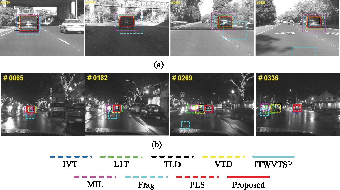
6.2.

Qualitative Evaluation

Qualitative analysis and discussions are provided as follows in common use of tracking human bodies, vehicles, and human and animal faces. The visual challenges include heavy occlusion, illumination change, scale change, fast motion, cluttered background, pose variation, motion blur, and low contrast.

6.2.1.

Human bodies

Tracking human bodies is widely used in motion-based recognition and automated surveillance. The sequences used for evaluation include Caviar 1, Caviar 2, and Singer.

It is shown in Fig. 5 that IVT,⁹ ITWVTSP,¹⁰ MIL,¹⁶ L1T,¹⁹ and PLS³⁸ do not perform well in Caviar 1. They fail to discover the target when it is occluded by a similar object (e.g., #0133 and #0192). Only the proposed tracker, VTD,²⁸ Frag,¹¹ and TLD¹⁷ handle the heavy occlusion successfully. However, VTD²⁸ and Frag¹¹ cannot smoothly adapt the scale changes of the person (e.g., #0133 and #0367). In Caviar 2, almost all the trackers evaluated except PLS³⁸ and MIL¹⁶ can follow the target. However, many of them including IVT,⁹ VTD,²⁸ ITWVTSP,¹⁰ and TLD¹⁷ cannot adapt the scale as the human moves near to the camera (e.g., #0220 and #0455). By contrast, our algorithm performs well in terms of position estimation and scale adaptation.

Fig. 5

Qualitative evaluation of (a) Caviar 1, (b) Caviar 2, and (c) Singer, where object appearances change drastically due to heavy occlusion, scale change, and light variation. Similar objects also appear in the scenes. Six patches are selected for the proposed algorithm.

In Singer shown in Fig. 5(c), only the results of partial trackers (e.g., proposed and VTD)²⁸ are satisfactory, while the others cannot adjust the scale [e.g., Frag,¹¹ L1T,¹⁹ and MIL¹⁶] or accurately locate the target [e.g., TLD¹⁷ at #098, #0116 and #0226, IVT⁹ at #0126]. Both drastic scale and location deviation occur when lighting condition changes. Especially, PLS³⁸ cannot capture the scale variation of the target through all the frames of Singer. The ITWVTSP¹⁰ algorithm performs much better than the IVT algorithm⁹ in this video. Comparatively, the proposed algorithms can locate the target more accurately and robustly against illumination variation.

6.2.2.

Human and animal faces

Face detection and tracking are very important in HCI and animal monitoring application. In the experiments, five videos are used including David Indoor, Occlusion 1, Occlusion 2, Girl, and Deer.

Figure 6 shows that in Occlusion 1, all the evaluation algorithms can follow the target approximately correctly, yet some trackers drift from the face when occlusion occurs [e.g., MIL¹⁶ at #0300, #0565, and #0833, ITWVTSP¹⁰ at #0565 and #0833, IVT,⁹ L1T,¹⁹ Frg,¹¹ TLD,¹⁷ and VTD²⁸ at #0565]. In Occlusion 2, the differences are more obvious. It can be found that L1T¹⁹ drifts more from the target compared with other algorithms [e.g., MIL¹⁶ at #0576, and #0713], and IVT⁹ and TLD¹⁷ cannot adapt the appearance during occlusion and head rotation (e.g., #0713). Though the VTD²⁸ and ITWVTSP¹⁰ could locate the face center more accurately, they could not cover the occluded area due to pose variation (e.g., #0713). PLS³⁸ cannot continuously follow the target, while MIL¹⁶ and Frag¹¹ estimate the target less accurately than the proposed algorithm.

Fig. 6

Qualitative evaluation of (a) Occlusion 1 and (b) Occlusion 2, where object appearances change drastically due to heavy occlusion and pose variation. Six patches are selected for the proposed algorithm.

In Girl, it is found in Fig. 7 that only the proposed algorithm, Frag,¹¹ TLD,¹⁷ and VTD²⁸ can consistently follow the face, while the proposed method can estimate the location more accurately (e.g., at #0310 and #0345). The other trackers gradually drift from the target to the surroundings. In David Indoor, some algorithms [e.g., Frag¹¹ and PLS³⁸] drift away from the target during the tracking process, while some algorithms cannot adapt the scale when out-of-plane rotation occurs [e.g., MIL¹⁶ and L1T¹⁹ at #0175 and #0389, VTD²⁸ and ITWVTSP¹⁰ at #00389]. In Deer, the successful trackers only include the proposed algorithms, VTD²⁸ and PLS,³⁸ while the others fail to capture the head of deer when it jumps up and down repeatedly. Comprehensively and qualitatively speaking, the proposed algorithms perform the best.

Fig. 7

Qualitative evaluation of (a) Girl, (b) David Indoor, and (c) Deer, where object appearances change drastically due to fast motion, pose variation, light variation, scale change, cluttered background and motion blur. Six patches are selected for the proposed algorithm.

6.2.3.

Vehicles

In vehicle navigation, especially self-driving technology, the basic role is to steadily track the rear of vehicles against different kinds of weather conditions and road environments. The sequences used for evaluation include Car 4 and Car 11, which are separately recorded in the day and at night. It is shown in Fig. 8 that Frag¹¹ and MIL¹⁶ do not perform well in the first two sequences. When the car goes into or out of the shadows, there is a drastic lighting change, which causes the estimated locations by VTD²⁸ and L1T¹⁹ to drift (e.g., at #0312 and #0429). The ITWVTSP¹⁰ tracker can locate the target center accurately but fails to adapt the scale change. In Car 11, only IVT,⁹ ITWVTSP,¹⁰ PLS,³⁸ and the proposed algorithm successfully track the target in the whole sequence. The remaining trackers drift away or take the surroundings as the target [e.g., MIL¹⁶ at #0182 and #0269 and VTD²⁸ and L1T¹⁹ at #0269 and #0336].

Fig. 8

Qualitative evaluation of (a) Car 4 and (b) Car 11, where object appearance changes drastically due to scale change, abrupt illumination variation, cluttered background, and low contrast. Six patches are selected for the proposed algorithm.

6.3.

Quantitative Evaluation

Besides qualitative evaluation, quantitative evaluation of the tracking results is also an important issue which typically computes the difference between the predicted and the manually labeled ground truth information. Similar with other classical works, two performance criteria are applied to compare the proposed tracker with other reference trackers. The first one refers to center error (CE) evaluation, which is the CE based on Euclidean distance from the tracking location to the ground truth center at each frame. The second one refers to the overlap ratio evaluation, which is also used in object detection³⁹ and defined as the share area proportion of the box obtained by tracker and the one by ground truth at each frame.

Furthermore, in this paper, the average CE (ACE) and average overlap rate (AOR) are introduced, which are defined as

Eq. (17)

ACE = \frac{1}{T} \sum_{i = 1}^{T} {‖ c_{eval}^{i} - c_{g t}^{i} ‖}_{2}^{2},

Eq. (18)

AOR = \frac{1}{T} \sum_{i = 1}^{T} \frac{A_{eval}^{i} \cap A_{g t}^{i}}{A_{eval}^{i} \cup A_{g t}^{i}},

where

c_{eval}^{i}, c_{g t}^{i} \in R^{2 \times 1}

refer to the horizontal and vertical center coordinates of the evaluation and ground-truth labeling results at the

i

’th frame, respectively, and

A_{eval}^{i}, A_{g t}^{i} \in R^{+}

are corresponding areas of the target in one test sequence.

The results of ACE and AOR for 10 sequences above are summarized in Table 2. For each sequence, the first line refers to ACE, whereas the second refers to AOR. It can be concluded that the proposed tracking method runs the best or the second-best performance on ACE and AOR in all the tested trackers. Though some CE values are higher, the gaps are limited, and all the AORs of proposed tracker except Car 4 are better than those of the others. Moreover, based on the ACE and AOR performance averages across all the experimental sequences, it can be concluded that the proposed performs comprehensively more favorably than the other methods. The details of the “center error” and “overlap rate” plot can be obtained from the authors.

Table 2

ACE (pixels) and average OR of tracking methods. The best two results are in bold and italics.

	Frag	IVT	VTD	L1T	TLD	MIL	ITWVTSP	PLS	Proposed
Caviar 1	5.699	45.245	3.909	119.932	5.593	48.499	42.342	47.393	1.197
Caviar 1	0.682	0.277	0.834	0.278	0.704	0.255	0.287	0.268	0.860
Caviar 2	5.569	8.641	4.724	3.243	8.514	70.269	4.569	32.431	1.784
Caviar 2	0.557	0.452	0.671	0.811	0.658	0.255	0.673	0.365	0.813
Singer	22.034	8.483	4.057	4.571	32.690	15.171	5.129	14.199	4.008
Singer	0.341	0.662	0.790	0.703	0.413	0.337	0.779	0.212	0.798
Occlusion 1	5.621	9.175	11.135	6.500	17.648	32.260	18.855	4.596	5.590
Occlusion 1	0.899	0.845	0.775	0.876	0.649	0.594	0.713	0.904	0.907
Occlusion 2	15.491	10.212	10.408	11.119	18.588	14.058	9.982	46.186	6.631
Occlusion 2	0.604	0.588	0.592	0.672	0.493	0.612	0.588	0.471	0.750
David Indoor	76.691	3.589	13.552	7.630	9.671	16.146	14.118	64.335	4.800
David Indoor	0.195	0.712	0.525	0.625	0.602	0.448	0.446	0.278	0.761
Deer	92.089	127.467	11.920	171.468	25.652	66.457	176.825	20.198	6.116
Deer	0.076	0.217	0.577	0.039	0.412	0.213	0.024	0.510	0.624
Girl	18.046	48.474	21.442	62.435	23.158	32.209	125.698	53.368	11.756
Girl	0.689	0.426	0.512	0.326	0.577	0.520	0.052	0.451	0.735
Car 4	179.775	2.866	12.290	4.081	18.797	60.104	7.831	10.163	3.991
Car 4	0.223	0.922	0.734	0.843	0.637	0.344	0.720	0.780	0.884
Car 11	63.922	2.106	27.055	33.252	25.113	43.465	2.066	1.691	2.048
Car 11	0.086	0.808	0.432	0.435	0.376	0.175	0.753	0.769	0.812
ACE average	51.877	35.656	14.372	46.776	18.542	39.864	40.450	29.456	4.795
AOR average	0.435	0.591	0.644	0.561	0.552	0.375	0.504	0.501	0.794

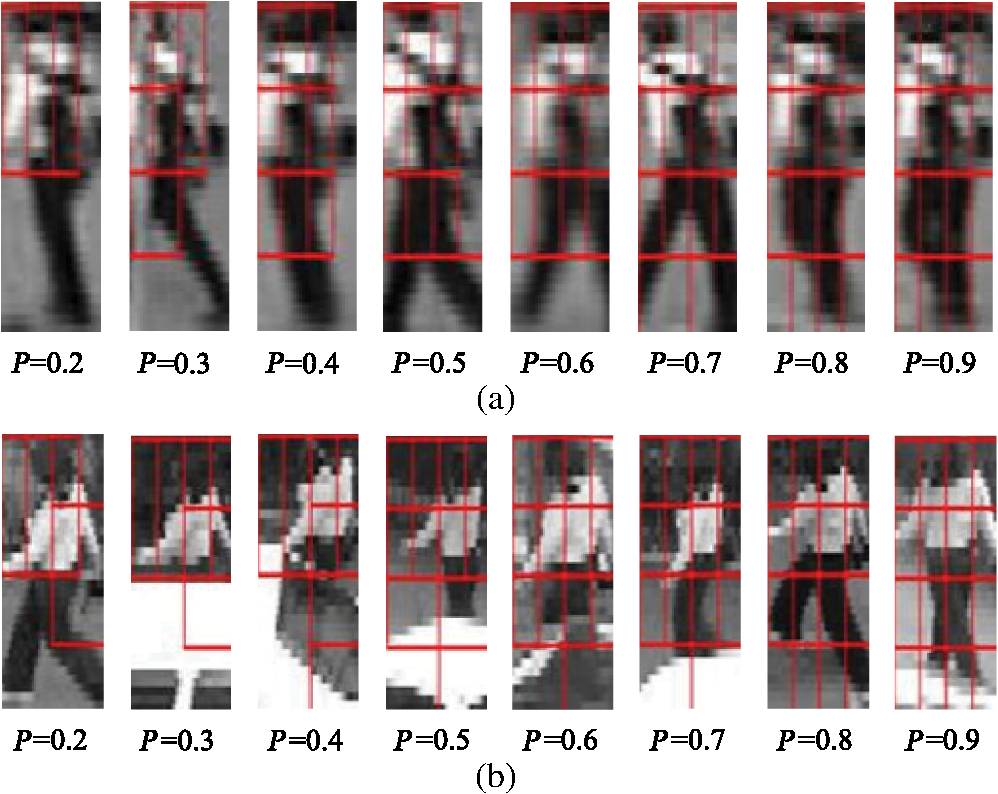
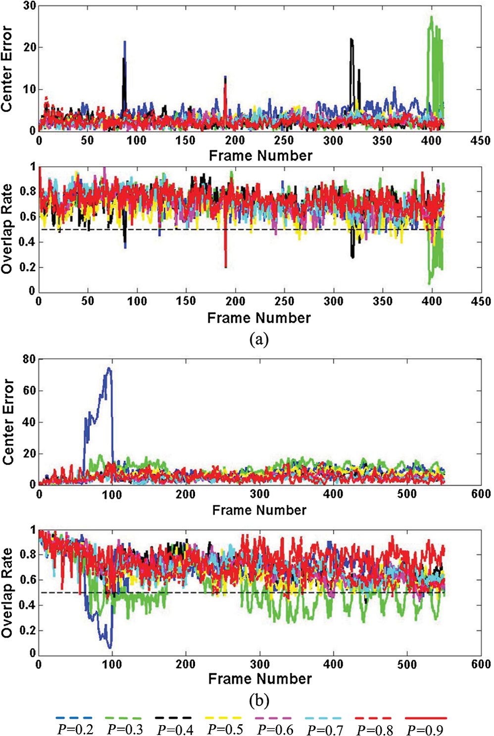
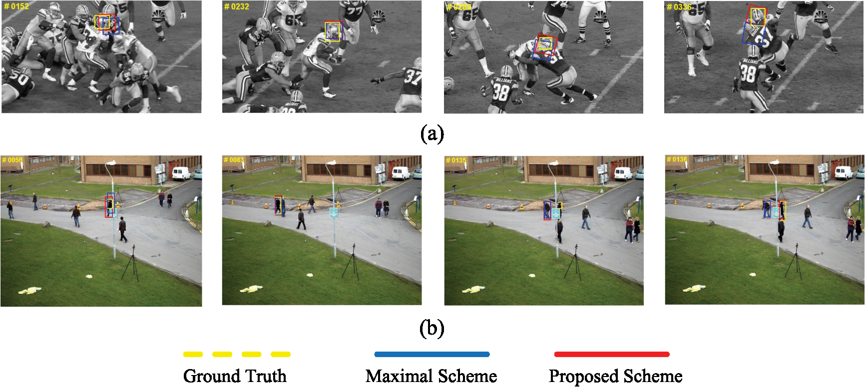
6.4.

Robustness on Patch Selection

The number of selected patches is one of the key issues related to tracking performance in the proposed algorithm. An experiment is conducted to evaluate its robustness. A number selection rate $P$ is introduced to fluctuate the selection number $K$ , $K = round (K_{0} \times P)$ , where $K_{0}$ refers to the patch number without selection, and $round (\cdot)$ is the approximation function. The rate $P$ varies from 0.2 to 0.9, while the other parameters are the same with the settings above. Two challenging sequences PETS2001²⁵ and Woman¹¹ are used.

Results of patch selection are shown in Fig. 9. Correspondingly, the CE and OR values are shown in Fig. 10. It is shown that the proposed tracker can generally follow the target with different selection rates rather than totally lose it. As $P$ decreases, the performance does not deteriorate much. It is obvious that too limited information of the target could prevent the tracker from uniquely and successfully modeling the target’s appearance, and thus the tracker fails to estimate the location with high accuracy. However, our proposed tracker could still find the likely location. Suppose a target is regarded as being successfully tracked when the OR is $> 0.5$ , a threshold line is added to the figure. Similar criterion is also applied in PASCAL VOC.³⁹ It is found in Fig. 10 that the proposed method is able to successfully track the target with limited selected patches, where $P$ is not $< 0.4$ empirically.

Fig. 9

Patch selection results with different $P$ values, which vary from 0.2 to 0.9. (a) PETS2001, (b) Woman.

Fig. 10

Center error (CE) and overlap rate (OR) with different $P$ values, which vary from 0.2 to 0.9. (a) PETS2001, (b) Woman.

6.5.

Comparison between Maximal and Proposed Inference Scheme

In Sec. 5.3, a geometric inference method is proposed to locate the target. Since the final target location would not be decided by the candidate with highest confidence score but with the inference output of highest candidates in CCS, it might affect the tracking accuracy. However, we argue that the influence is quite limited, and more favorable performance compared with other works has been obtained as described above. More importantly, the proposed scheme is quite useful in cluttered background and complete occlusion environment when it is integrated with covariance variation in dynamic modeling. Heuristically, it could be viewed as a soft and local abnormality detection scheme. In cluttered background, the tracker is subject to the target’s outside distraction. Under the motion continuity assumption, the proposed scheme obtains spatial cues from the most confident candidates to stabilize and centralize the location. In the complete occlusion situation, the scheme provides extra opportunities to detect the target in a wider area. To demonstrate such characteristics and advantages over the maximal scheme, two challenging sequences Football²⁸ and Pets2009⁴⁰ are used.

The selected qualitative results are shown in Fig. 11. In Fig. 11(a) on sequence Football, it is found that without geometric inference, the tracker gradually drifts to the surrounding areas of the player’s head due to the neighborhood similarity (e.g., #0289 and #336), while more stable performance is obtained with the proposed geometric inference scheme. The sequence Pets2009 is quite challenging; because when the target is heavily occluded, another pedestrian is passing by him. The tracker with the maximal scheme eventually follows a wrong object. In the proposed method, although the tracker mistakes the wrong pedestrian for the target in the first several frames, sparse coefficients of the false target would scatter the points distribution in the CCS, violate the inference condition, and cause the sampling state ${\tilde{X}}_{t}$ to be much biased. Based on these unacceptable inference results, the searching range is extended according to Algorithm 2. When the true target appears again without much appearance variation, the tracker re-detects it and continues with correct location estimation in the following sequences.

Fig. 11

Geometric inference comparison between maximal and proposed scheme. (a) Football, (b) PETS2009.

6.6.

Computational Complexity Analysis

In Sec. 5, it could be found that sparse coding and the proposed spatial confidence inference algorithm are most time consuming. Thus, we also compare the computation complexity and processing time with three representative trackers including IVT,⁹ ITWVTSP,¹⁰ and L1T which is show in Table 3.¹⁹ Suppose $d$ refers to the dimension of a vectorized image, and $M$ is the number of eigen vectors or templates, $d ≫ M$ , the computational complexity of IVT⁹ and ITWVTSP¹⁰ is $O (d M)$ , for they mainly involve matrix–vector multiplication. The computational load of L1T¹⁹ is $O (d^{2} + d M)$ , while the load of the proposed algorithm is $O (K s M + 9 Q M)$ . The first part is related to sparse coding, where $K$ refers to the number of selected patches, and $s$ is the patch size, $d^{2} ≫ K s > d$ . The second part is related to geometric inference, $Q$ is inference point number, $M < 9 Q M ≪ d$ . Moreover, processing times of different normalized image sizes ( $16 \times 16$ and $32 \times 32$ ) for solving one image are also presented. It can be found that enlarging the normalized size of the target region increases the computation time. Both the L1T¹⁹ algorithm and the proposed one apply sparse representation and yet the proposed tracker is much faster than the L1T¹⁹ tracker. Although the proposed algorithm is slower than the IVT⁹ and ITWVTSP¹⁰ algorithm, it achieves a better performance in accuracy evaluation.

Table 3

Computation complexity and processing time (seconds) of tracking methods.

Algorithm	Computational Complexity	Time ( $16 \times 16$ )	Time ( $32 \times 32$ )
IVT	$O (d M)$	0.019 s	0.074 s
ITWVTSP	$O (d M)$	0.021 s	0.076 s
LIT	$O (d^{2} + d M)$	0.320 s	0.842 s
Proposed	$O (K s M + 9 Q M)$	0.247 s	0.535 s

7. Conclusion

This paper presents a generative tracking algorithm based on sparse representation of selected overlapped patches via KPPR and spatiotemporal geometric inference of candidate confidences sampled by propagated affine motion modeling. Not only qualitative and quantitative evaluations but also the analysis on selected patch number and geometric inference process are conducted. The experiments demonstrate that on challenging image sequences, our proposed tracking algorithm comprehensively performs more favorably against state-of-the-art online tracking algorithms. The future work might include exploring more efficient $l_{1}$ minimization algorithms (e.g., APG)³² for real-time application and extending this algorithm to multiple-object tracking given certain application environments. Currently, the temporal weight matrix in Eq. (10) is fixed during the tracking process. More information could be introduced for its adaption to the latest tracking conditions.

Acknowledgments

This work is supported by NSFC (No. 61171172 and No. 61102099), National Key Technology R&D Program (No. 2011BAK14B02), and STCSM (No. 10231204002, No. 11231203102 and No. 12DZ2272600). We acknowledge Dr. Javier Cruz-Mota and the other authors for sharing the source codes of evaluated trackers. We also give our sincere thanks to the anonymous reviewers for their comments and suggestions.

References

1.

A. YilmazO. JavedM. Shah, “Object tracking: a survey,” ACM Comput. Surv., 38 1 –45 (2006). http://dx.doi.org/10.1145/1177352 ACSUEY 0360-0300 Google Scholar

2.

M. IsardA. Blake, “Condensation - conditional density propagation for visual tracking,” Int. J. Comput. Vision, 29 (1), 5 –28 (1998). http://dx.doi.org/10.1023/A:1008078328650 IJCVEQ 0920-5691 Google Scholar

3.

I. HaritaogluD. HarwoodL. S. Davis, “W4: real-time surveillance of people and their activities,” IEEE Trans. Pattern Anal. Mach. Intell., 22 (8), 809 –830 (2000). http://dx.doi.org/10.1109/34.868683 ITPIDJ 0162-8828 Google Scholar

4.

P. Pérezet al., “Color-based probabilistic tracking,” in Proc. 7th European Conference on Computer Vision-Part I, 661 –675 (2002). Google Scholar

5.

Q. Wanget al., “An experimental comparison of online object-tracking algorithms,” Proc. SPIE, 8138 81381A (2011). http://dx.doi.org/10.1117/12.895965 PSISDG 0277-786X Google Scholar

6.

M. Arulampalamet al., “A tutorial on particle filters for online nonlinear/non-gaussian bayesian tracking,” IEEE Trans. Signal Process., 50 (2), 174 –188 (2002). http://dx.doi.org/10.1109/78.978374 ITPRED 1053-587X Google Scholar

7.

S. SaltiA. CavallaroL. Di Stefano, “Adaptive appearance modeling for video tracking: survey and evaluation,” IEEE Trans. Image Process., 21 4334 –4348 (2012). http://dx.doi.org/10.1109/TIP.2012.2206035 IIPRE4 1057-7149 Google Scholar

8.

J. ShiC. Tomasi, “Good features to track,” in 1994 IEEE Conf. Computer Vision and Pattern Recognition (CVPR’94), 593 –600 (1994). Google Scholar

9.

D. A. Rosset al., “Incremental learning for robust visual tracking,” Int. J. Comput. Vision, 77 (1–3), 125 –141 (2008). http://dx.doi.org/10.1007/s11263-007-0075-7 IJCVEQ 0920-5691 Google Scholar

10.

J. Cruz-MotaM. BierlaireJ. Thiran, “Sample and pixel weighting strategies for robust incremental visual tracking,” IEEE Trans. Circuits Syst. Video Technol., 23 (5), 898 –911 (2013). http://dx.doi.org/10.1109/TCSVT.2013.2249374 ITCTEM 1051-8215 Google Scholar

11.

A. AdamE. RivlinI. Shimshoni, “Robust fragments-based tracking using the integral histogram,” in 2006 IEEE Computer Society Conf. Computer Vision and Pattern Recognition (CVPR 2006), 798 –805 (2006). Google Scholar

12.

M. YangJ. YuanY. Wu, “Spatial selection for attentional visual tracking,” in IEEE Conf. Computer Vision and Pattern Recognition, 1 –8 (2007). Google Scholar

13.

Y. ZhouH. SnoussiS. Zheng, “Bayesian variational human tracking based on informative body parts,” Opt. Eng., 51 (6), 067203 (2012). http://dx.doi.org/10.1117/1.OE.51.6.067203 OPEGAR 0091-3286 Google Scholar

14.

H. GrabnerH. Bischof, “On-line boosting and vision,” in IEEE Computer Society Conf. Computer Vision and Pattern Recognition, 260 –267 (2006). Google Scholar

15.

H. GrabnerC. LeistnerH. Bischof, “Semi-supervised on-line boosting for robust tracking,” in Proc. 10th European Conf. Computer Vision: Part I, 234 –247 (2008). Google Scholar

16.

B. BabenkoM.-H. YangS. Belongie, “Robust object tracking with online multiple instance learning,” IEEE Trans. Pattern Anal. Mach. Intell., 33 1619 –1632 (2011). http://dx.doi.org/10.1109/TPAMI.2010.226 ITPIDJ 0162-8828 Google Scholar

17.

Z. KalalK. MikolajczykJ. Matas, “Tracking-learning-detection,” IEEE Trans. Pattern Anal. Mach. Intell., 34 (7), 1409 –1422 (2012). ITPIDJ 0162-8828 Google Scholar

18.

S. Wanget al., “Superpixel tracking,” in IEEE Int. Conf. Computer Vision, 1323 –1330 (2011). Google Scholar

19.

X. MeiH. Ling, “Robust visual tracking and vehicle classification via sparse representation,” IEEE Trans. Pattern Anal. Mach. Intell., 33 (11), 2259 –2272 (2011). http://dx.doi.org/10.1109/TPAMI.2011.66 ITPIDJ 0162-8828 Google Scholar

20.

B. Liuet al., “Robust tracking using local sparse appearance model and k-selection,” in IEEE Conf. Computer Vision and Pattern Recognition, 1313 –1320 (2011). Google Scholar

21.

H. LiC. ShenQ. Shi, “Real-time visual tracking using compressive sensing,” in IEEE Conf. Computer Vision and Pattern Recognition, 1305 –1312 (2011). Google Scholar

22.

J. KwonK. M. LeeF. Park, “Visual tracking via geometric particle filtering on the affine group with optimal importance functions,” in IEEE Conf. Computer Vision and Pattern Recognition, 991 –998 (2009). Google Scholar

23.

A. JepsonD. FleetT. El-Maraghi, “Robust online appearance models for visual tracking,” IEEE Trans. Pattern Anal. Mach. Intell., 25 (10), 1296 –1311 (2003). http://dx.doi.org/10.1109/TPAMI.2003.1233903 ITPIDJ 0162-8828 Google Scholar

24.

S. K. ZhouR. ChellappaB. Moghaddam, “Visual tracking and recognition using appearance-adaptive models in particle filters,” IEEE Trans. Image Process., 13 (11), 1491 –1506 (2004). http://dx.doi.org/10.1109/TIP.2004.836152 IIPRE4 1057-7149 Google Scholar

25.

X. Meiet al., “Minimum error bounded efficient l1 tracker with occlusion detection,” in IEEE Conf. Computer Vision and Pattern Recognition, 1257 –1264 (2011). Google Scholar

26.

T. BaiY. Li, “Robust visual tracking with structured sparse representation appearance model,” Pattern Recognit., 45 (6), 2390 –2404 (2012). http://dx.doi.org/10.1016/j.patcog.2011.12.004 PTNRA8 0031-3203 Google Scholar

27.

X. JiaH. LuM.-H. Yang, “Visual tracking via adaptive structural local sparse appearance model,” in IEEE Conf. Computer Vision and Pattern Recognition, 1822 –1829 (2012). Google Scholar

28.

J. KwonK.-M. Lee, “Visual tracking decomposition,” in IEEE Conf. Computer Vision and Pattern Recognition, 1269 –1276 (2010). Google Scholar

29.

X. Liet al., “Visual tracking via incremental log-Euclidean riemannian subspace learning,” in IEEE Conf. Computer Vision and Pattern Recognition, 1 –8 (2008). Google Scholar

30.

J. Wrightet al., “Robust face recognition via sparse representation,” IEEE Trans. Pattern Anal. Mach. Intell., 31 (2), 210 –227 (2009). http://dx.doi.org/10.1109/TPAMI.2008.79 ITPIDJ 0162-8828 Google Scholar

31.

M. Elad, Sparse and Redundant Representations: From Theory to Applications in Signal and Image Processing, 1st ed.Springer Publishing Company, Inc., Berlin, Heidelberg (2010). Google Scholar

32.

C. Baoet al., “Real time robust l1 tracker using accelerated proximal gradient approach,” in IEEE Conf. Computer Vision and Pattern Recognition, 1830 –1837 (2012). Google Scholar

33.

H. ZouT. Hastie, “Regularization and variable selection via the elastic net,” J. R. Stat. Soc. Ser. B, 67 (2), 301 –320 (2005). http://dx.doi.org/10.1111/rssb.2005.67.issue-2 JSTBAJ 0035-9246 Google Scholar

34.

J. Mairalet al., “Online learning for matrix factorization and sparse coding,” J. Mach. Learn. Res., 11 (2), 19 –60 (2010). 1532-4435 Google Scholar

35.

C. E. RasmussenC. K. I. Williams, Gaussian Processes for Machine Learning (Adaptive Computation and Machine Learning), MIT Press, Cambridge, MA (2005). Google Scholar

36.

B. Efronet al., “Least angle regression,” Ann. Stat., 32 (2), 407 –499 (2004). http://dx.doi.org/10.1214/009053604000000067 ASTSC7 0090-5364 Google Scholar

37.

M. XueS. Zheng, “A bayesian online object tracking method using affine warping and random kd-tree forest,” Multimedia and Signal ProcessingCommunications in Computer and Information Science, 275 –282 Springer, Berlin, Heidelberg (2012). Google Scholar

38.

Q. Wanget al., “Object tracking via partial least squares analysis,” IEEE Trans. Image Process., 21 (10), 4454 –4465 (2012). http://dx.doi.org/10.1109/TIP.2012.2205700 IIPRE4 1057-7149 Google Scholar

39.

M. Everinghamet al., “The pascal visual object classes (voc) challenge,” Int. J. Comput. Vision, 88 (2), 303 –338 (2010). http://dx.doi.org/10.1007/s11263-009-0275-4 IJCVEQ 0920-5691 Google Scholar

40.

J. SanMiguelA. CavallaroJ. Martinez, “Adaptive online performance evaluation of video trackers,” IEEE Trans. Image Process., 21 (5), 2812 –2823 http://dx.doi.org/10.1109/TIP.2011.2182520 IIPRE4 1057-7149 Google Scholar

Biography

Ming Xue received his BE degree from Shanghai University, Shanghai, China, in 2007 and his MS degree from Xidian University, Xi’an, China, in 2010. He is currently working toward the PhD degree in information and communication engineering from Shanghai Jiaotong University, Shanghai, China. From 2008 to 2009, he was a visiting student at Israel Institute of Technology (Technion), Haifa, Israel, sponsored by Chinese-Israel Governmental Exchange Scholarship. His current research interests include intelligent surveillance, multimedia systems, and machine learning.

Shibao Zheng received both the BS and MS degrees in electronic engineering from Xidian University, Xi’an, China, in 1983 and 1986, respectively. He is currently the professor and vice director of Elderly Health Information and Technology Institute of Shanghai Jiao Tong University (SJTU), Shanghai, China. His current research interests include urban image surveillance system, intelligent video analysis, spatial information system, and elderly health technology, etc.

Hua Yang received her PhD degree in communication and information from Shanghai Jiaotong University, in 2004, and both the BS and MS degrees in communication and information from Haerbin Engineering University, China, in 1998 and 2001, respectively. She is currently an associate professor in the Department of Electronic Engineering, Shanghai Jiaotong University, China. Her current research interests include video coding and networking, machine learning, and smart video surveillance.

Yi Zhou received his PhD degree in information and communication engineering from both Shanghai Jiaotong University and University of Technology of Troyes, France, in 2012, and both the BS and MS degrees in electronic engineering from Dalian Maritime University, Dalian, China, in 2003 and 2006. He is currently a lecturer in the Department of Electronics Engineering, Dalian Maritime University. His research interests include signal processing, computer vision, and machine learning.

Zhenghua Yu received his BEng and MEng from Southeast University, China, in 1993 and 1996, respectively. He received the PhD in pattern recognition and intelligent control from Shanghai Jiaotong University in 1999. He held senior research positions at Motorola Labs, Sydney, and National ICT Australia from 2000 to 2006. He is currently the chief scientist of Bocom Smart Network Technologies Inc. His current research interests include computer vision, machine learning, image and video processing, and their industrial applications.

CC BY: © The Authors. Published by SPIE under a Creative Commons Attribution 4.0 Unported License. Distribution or reproduction of this work in whole or in part requires full attribution of the original publication, including its DOI.

Citation Download Citation

Ming Xue, Shibao Zheng, Hua Yang, Yi Zhou, and Zhenghua Yu "Online visual tracking based on selective sparse appearance model and spatiotemporal analysis," Optical Engineering 53(1), 013103 (23 January 2014). https://doi.org/10.1117/1.OE.53.1.013103

Published: 23 January 2014

Access the abstract

JOURNAL ARTICLE
16 PAGES

DOWNLOAD PAPER SAVE TO MY LIBRARY