|
|
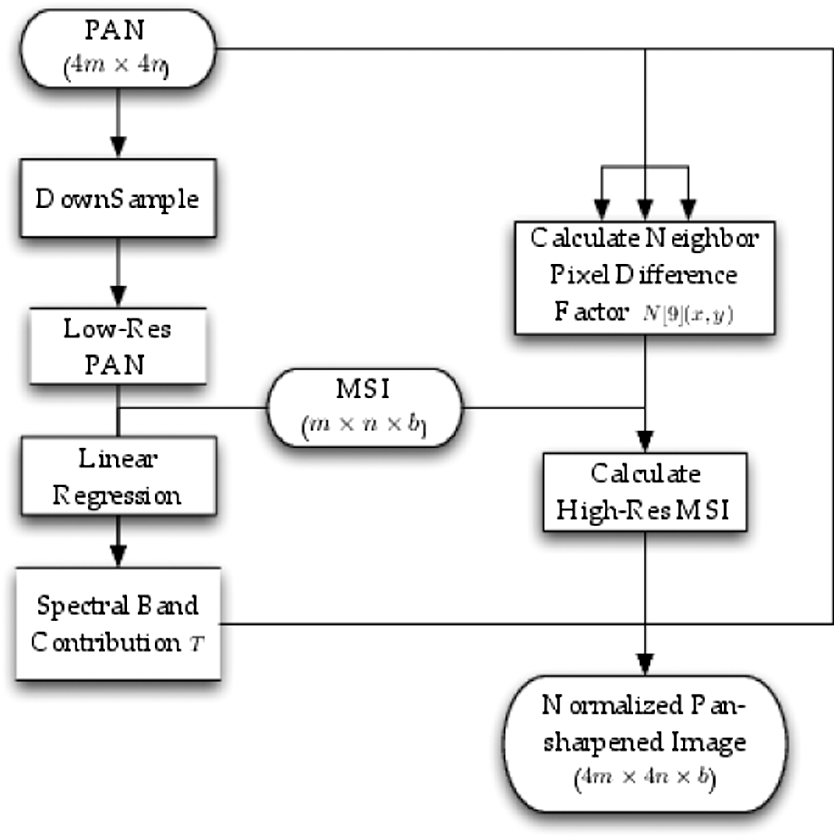
1.IntroductionModern space-borne imaging sensors deliver high-spectral resolution multispectral [multispectral spectral image (MSI)] as well as corresponding high-spatial resolution panchromatic images. While one can choose between the two sets of images based on the application, the tradeoff between spectral and spatial resolutions has existed for decades. Recently, several applications, such as feature extraction, image segmentation, change detection, and land-cover classification, require both spatial and spectral images for detection of fine features in suburban or urban scenes. For example, in building detection, a typical residential 43-ft wide house occupies fewer than 7 pixels on one side (at 2-m resolution in the MSI), which makes it very difficult for detection algorithms to discern salient line or edge features. While the current instruments are not capable of providing both spatial and spectral high-resolution images either by design or by observational constraints, pan-sharpening can well serve as a tool to fuse the MSI and panchromatic images. The literature shows a large collection of pan-sharpening methods developed,1–7 and recent reviews can be found in Refs. 89.–10. The existing methods can be roughly categorized into three groups: component substitution (CS) method,11–13 relative spectral contribution (RSC) method,14,15 and multiresolution (MR) method.16–19 More detailed categorizations are surveyed in Refs. 8–10. The CS method substitutes a high-resolution image for the selected band after spectral transformation. The RSC methods increase the spatial details through arithmetical calculations with the panchromatic image. The MR methods, based on wavelet decompositions and Laplacian pyramids, inject high-frequency components to each band of the MSI. Various methods have been proposed based on this framework to reduce spatial and spectral distortions such as context-based decision injection,16 mean-square-error minimization,18 and the introduction of sensor spectral response.20 However, these approaches enhance the image by adding details to each multispectral band weighted by certain coefficients separately, which is by nature a band-by-band process. Furthermore, they assume a correlation between the PAN and each MS band. Such an assumption may not hold for some spectral bands such as the near infrared band (NIR-2) for WorldView-2 images, which has no spectral overlap with the PAN band.21 Among the existing methods, some of them have been shown to produce very high-quality fused imagery such as Gram–Schmidt method,22 generalized minimum mean-square-error (gMMSE) method,18 and University of New Brunswick (UNB) sharpening method.13 The Gram–Schmidt method is a multivariate statistics-based approach. It is patented by Kodak and widely used in many commercial image-processing packages. The gMMSE method is an optimized, MR analysis-based approach that uses general Laplacian pyramid. The gMMSE method injects higher frequency resolution from the PAN to the MSI and minimizes the root mean squared errors by optimizing fusion parameters through enhancing a degraded version of the MSI and the PAN. The authors of gMMSE claim to produce very satisfactory results that outperform the winner of the IEEE Data Fusion Contest of 2006.23 The UNB method is a proprietary algorithm and can be classified as a CS-based statistical approach.23 The method has been shown to produce a pan sharpened image of very high spatial quality.24 In this article, a novel pan-sharpening method is proposed which uses the pixel spectrum as its smallest unit of operation and generates resolution-enhanced spectral images using a mixture model. The underlying assumption of our approach is that each new spectrum in the high-resolution fused image is a weighted combination of the immediate neighboring superpixel spectra in the low-resolution spectral image. The weights are controlled by a diffusion model inferred from the panchromatic image that relates the similarity of the pixel of interest to the neighboring superpixels. The per-pixel-spectrum operation nature is different from the existing algorithms, which mostly rely on a band-by-band processing. The results show that our algorithm is capable of preserving very sharp spatial features indiscernible from the multispectral images while preserving spectral information from multispectral images. This is particularly important for applications (such as land-cover classification) that rely on accurate spectral information beyond traditional visual inspection. In addition, our approach is fairly straightforward and highly parallel. It can be implemented using OpenMP and compute unified device architecture (CUDA) parallel processing techniques, which significantly reduces the processing time to a satisfactory timeframe. This article is organized as follows. Section 2 introduces the algorithm for our nearest-neighbor diffusion-based pan-sharpening method. The results of our method are shown in Sec. 3 together with a discussion of comparison with state-of-the-art algorithms. Finally, we provide a discussion and future work in Sec. 4. 2.MethodThe pan-sharpening algorithm follows the flowchart shown in Fig. 1. The algorithm works in two branches. In the left branch of Fig. 1, a spectral band photometric contribution vector is obtained through linear regression. The vector is of size , where is the number of MSI bands. It relates the contribution of the digital counts of each multispectral band to the panchromatic image. We assume where is the digital count of pixel in the downsampled PAN, is the ’th value in vector , is the digital count of corresponding pixel in the ’th band of MSI, and accounts for regression error. This assumption is valid, since the spectral response function of each single band in MSI does not overlap much with each other and that the ensemble of all MSI bands can cover the spectral range of the PAN in general. In practice, if certain MSI bands do not overlap with the PAN spectral bandwidth, for these bands should be zero or very close to zero. Since PAN and MSI are not of the same spatial size, to obtain , we need to downsample the PAN to fit the size of the MSI and then perform the linear regression. The vector is useful in the following steps to normalize the spectral values. can also be obtained from the sensor spectral radiance responses.21In the other branch of the flowchart, the difference factors from neighboring superpixels are acquired for each pixels from the PAN at the original resolution. The factors are calculated from where defines the diffusion region for each of the nine neighboring superpixels as shown in Fig. 2, and denotes the position of a pixel in the high-resolution coordinate. The fundamental idea of the difference factor is to reflect the difference of the pixel of interest in the PAN to each of its neighboring superpixels. The difference factors estimate the similarity of the pixel of interest to its nine superpixels by comparing a summation of difference. A zero indicates that the ’th superpixel (counted in a row-major fashion) is the same as pixel and that a strong diffusion should happen; on the other hand, a high value suggests that is very different from the ’th superpixel; thus there should be a very restricted diffusion. It is worth mentioning that the integration areas in Fig. 2 include not only the superpixel itself, but also a few connecting pixels from the pixel of interest to the superpixel. These pixels are introduced to account for cases when a strong edge is located on the connecting pixels but not inside the superpixels, which should indicate a signal of a weak diffusion. The summation over the connected pixels will avoid such unwarranted diffusion. In the ideal case, the difference factor should be calculated as a summation of the shortest geodesic distance from the point of interest to each pixel in the superpixels, but this will require sophisticated optimization techniques such as ant colony optimization;25,26 Eq. (2) poses as a valid approximation to this ideal case, since the diffusion areas are fairly small. In addition, the estimation can significantly reduce the computation time. It is worth mentioning that the integration regions are not only suitable for resolution scale, but also applicable to any integer resolution scale as well. The general rule for mapping the integration regions is to cover the ’th superpixel as well as the center subpixels leading to that superpixel. Although there is no rigorous physical evidence to support such mapping scheme, it is consistent with our intuition and has been empirically tested to perform very well in various scenarios.Fig. 2Illustrations for calculating the difference factors. The integration regions (shaded pixels) for the pixel of interest (blue) are shown for the nine nearest-neighboring superpixels (denoted by the grids enclosed in the thick borders). 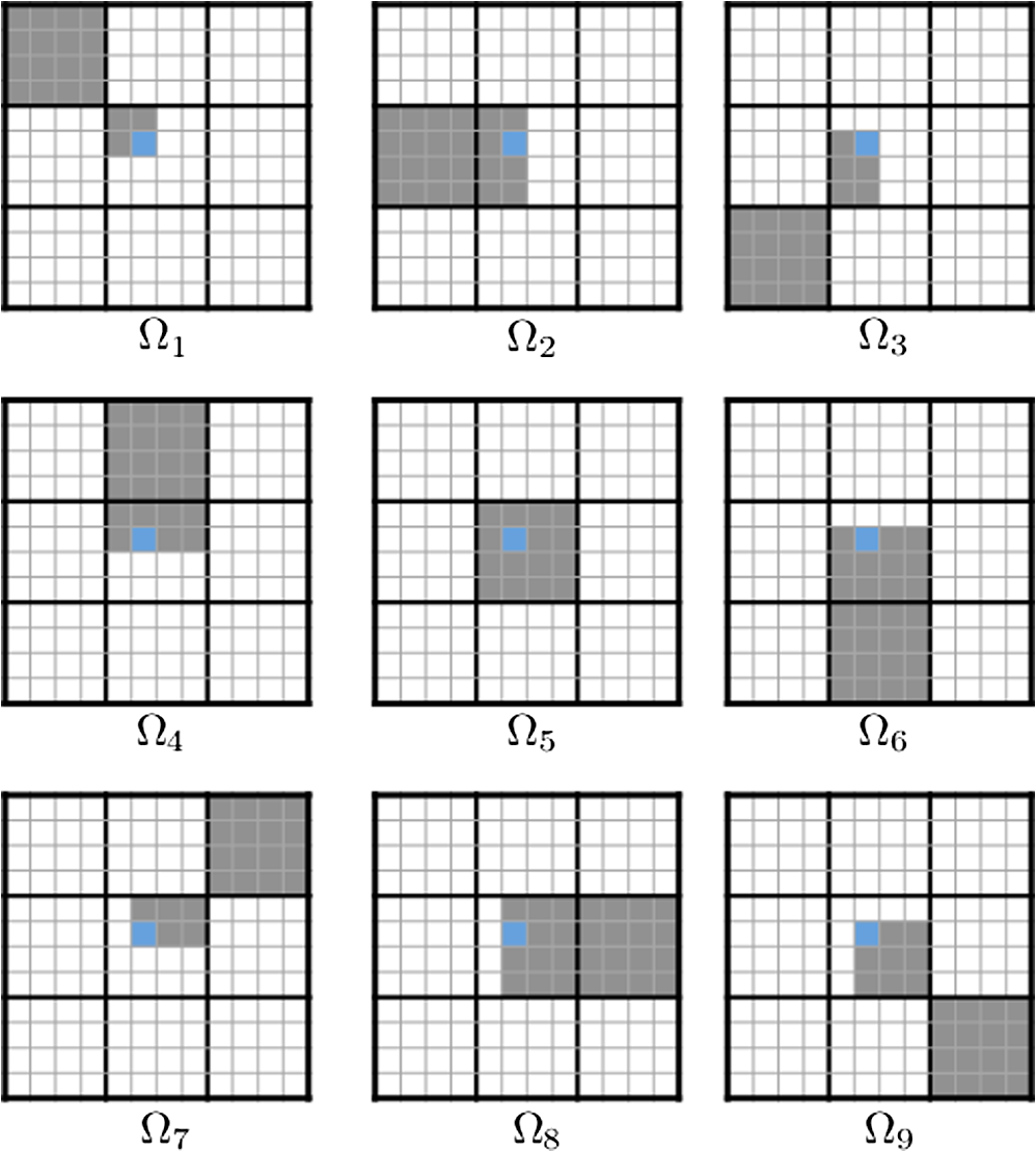 provides a similarity metric between pixel to its neighboring superpixels. It is then possible to generate the new spectrum simulating the problem of anisotropic diffusion27 as where is the spectrum vector of neighboring superpixels corresponding to pixel , and is in accordance with diffusion regions illustrated in Fig. 2. and are the center pixel locations of the nine neighboring superpixels . and are the intensity (range) and spatial smoothness factors that control the sensitivity of the diffusion, respectively. Equation (3) relates diffusion factors to a multiplication of pixel value similarity and spatial closeness. Inside the summation, gives a similarity measure between pixel and its neighboring superpixels, whereas provides a spatial closeness measure of pixel to the center of the neighboring superpixels. is a normalization factor calculated as so that where is obtained from the linear regression by Eq. (1). The pan-sharpened image will resemble the PAN, in which it preserves the gradient information from the PAN. The algorithm also uses a linear mixture model as shown in Eq. (3), so that a spectrum in the MSI is the smallest element of operation. The linear mixture model reduces color distortion and preserves spectral integrity.3.ResultsOur algorithm has been implemented to work with no sensor dependency. In this article, we tested our algorithm on a number of WorldView-2, GeoEye-1, and USGS EO-1 sensor images. These scenes are summarized in Table 1. The spatial smoothness factor is set to 2.5 for spatial ratio and 1.9 for spatial ratio. The intensity factor is set adaptively using local similarity, so that where is the difference factor of the nine neighbors given by Eq. (2). A discussion for the proper choice of and is provided in Sec. 6.Table 1Description of the dataset used in this article.28–31
3.1.Spatial AnalysisThe first test scene is a WorldView-2 image of a parking area in Rochester, New York, captured from June 2009 shown in Fig. 3. The scene is very complex, in which it comprises abundant objects (roads, vegetation, houses, and cars) and a great number of them are fairly small. We performed the fusion technique described in Sec. 2. The spectral band contribution vector is fitted from linear regression using all the pixels across the entire scene and is shown in Table 2. In this step, the PAN image is downsampled to match the spatial size of the MSI; thus the regression can be carried out using all the pixels in the downsampled PAN and the MSI. The error is calculated as the root mean squared error over the mean value of the PAN. Since is obtained through linear regression, it may not exactly reflect the contribution of each multispectral band to the panchromatic band; but the values in Table 2 show that the digital counts in PAN are mostly contributed from the blue to the red edge bands, which is consistent with the spectral radiance response of the WorldView-2 sensor.21 Although we see a slight negative contribution from the Coastal band, the value is fairly small and does not appear to have any effect on our final results. Fig. 3Parking area scene. Panchromatic image is shown in (a), the RGB bands are shown in (b), and the color-IR in (c) with nearest-neighbor interpolation. 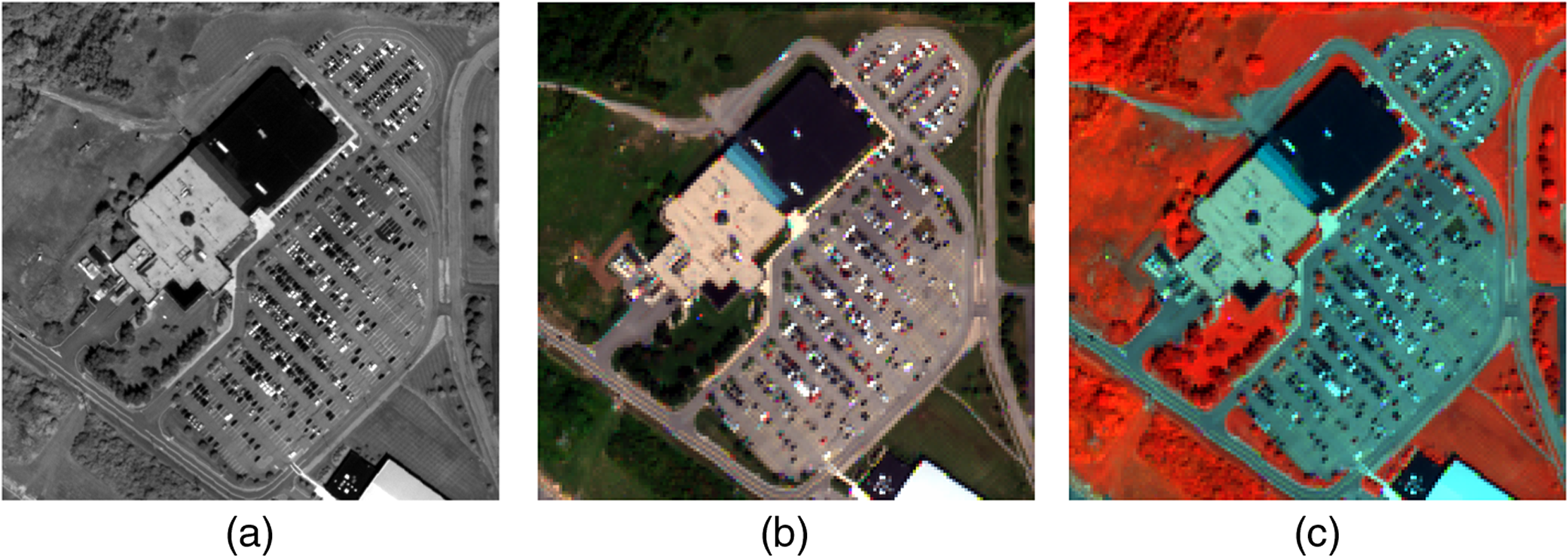 Table 2The spectral band contribution vector for the parking area scene.
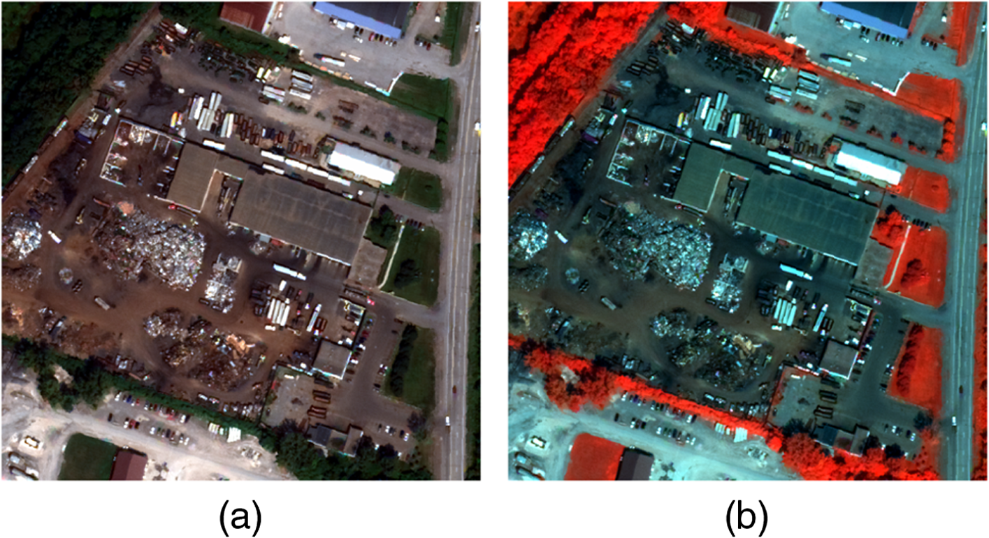
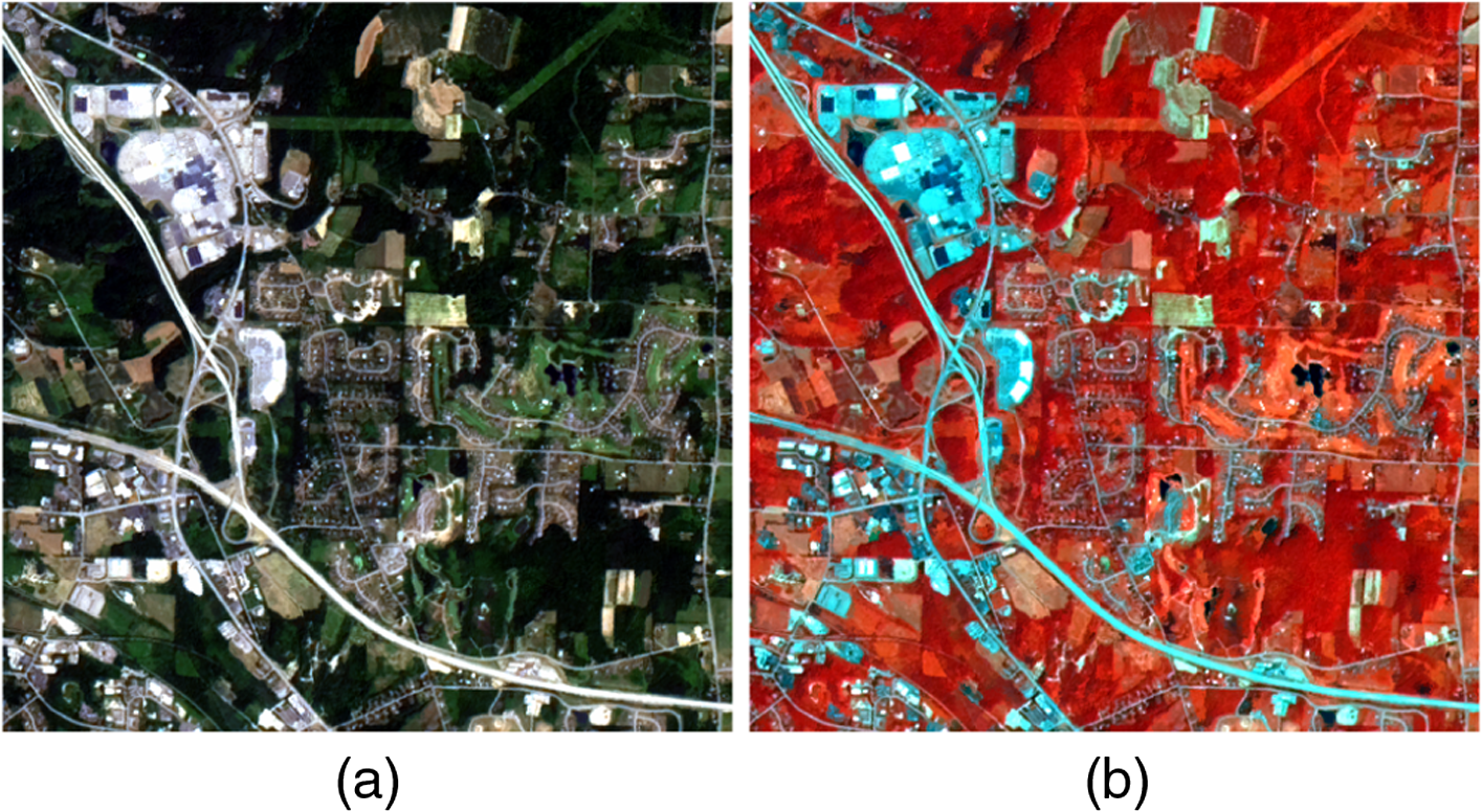
The synthesized image of our diffusion-based pan-sharpening approach is shown in Fig. 4, where the RGB bands and the color-IR bands are displayed and their histograms are matched with the images shown in Fig. 3 for visual comparison. The pan-sharpened images show good spatial and color quality. The algorithm preserves the strong edges well in both the PAN and the MSI. One can clearly see the cars and the parking lane marks as well as the edges of the buildings. The RGB colors in the MSI are well maintained for the uniform areas such as the building rooftops and the parking spots. The color-IR image also indicates that our method works not only for RGB, but also for other bands as well. Fig. 4The pan-sharpened image [RGB bands (a) and color-IR (b)] of the parking area scene. The image histograms are matched with the MSI in Fig. 3. 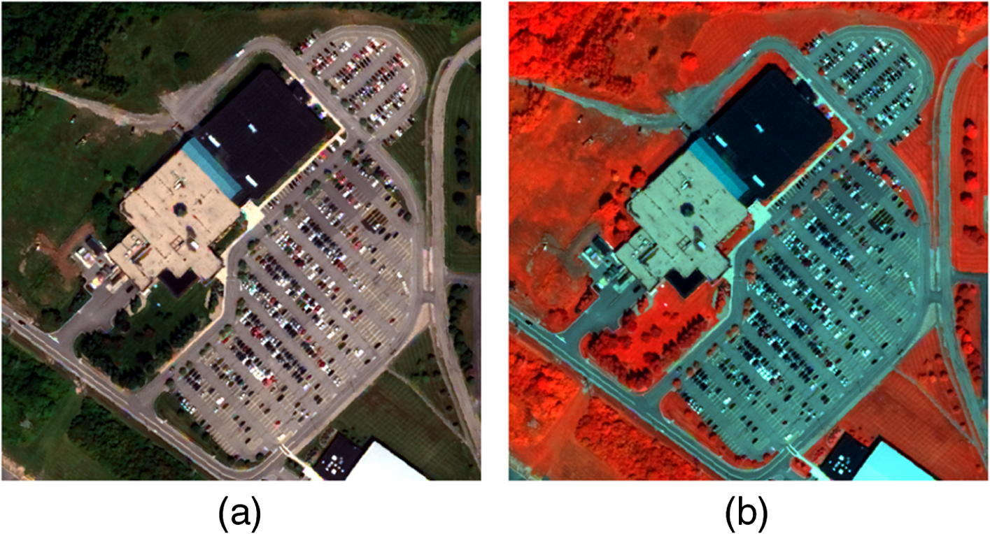 The second test scene is a recycling site also from the WorldView-2 sensor. The PAN, RGB, and color-IR from the MSI are shown in Fig. 5. This site possesses a lot of fine spatial details. The pan-sharpening result is shown in Fig. 6. Similar to the results of the parking site scene, the image preserves well the spatial details with very accurate spectral/color information. Fig. 5Recycling site scene from WorldView-2 Imagery. (a) Panchromatic image, (b) original MSI RGB bands, and (c) original MSI color-IR bands. 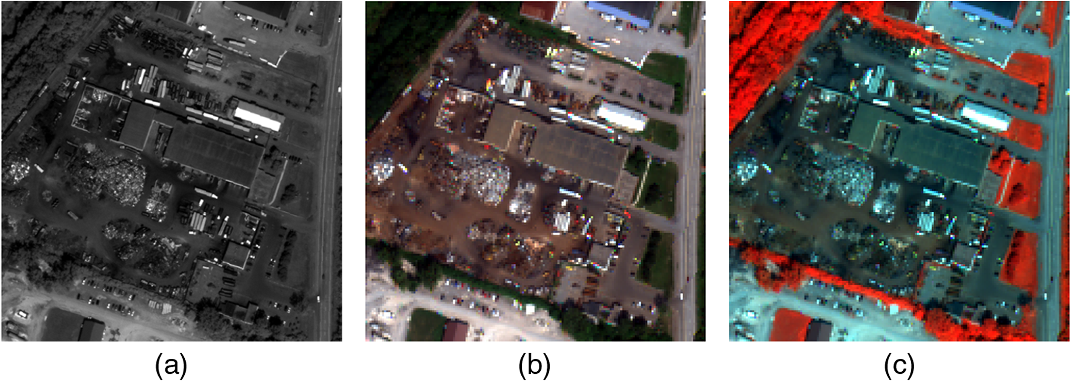 We also tested our algorithm on a GeoEye-1 sensor image of Rome, Italy, shown in Fig. 7. The imagery is composed of four bands covering visible and near-infrared. This scene contains rich structural details in the Colosseum and the building complexes. The pan-sharpened image is shown in Fig. 8. The spectral band contribution vector, obtained through linear regression, shows that the PAN band correlates mostly with the green and red bands, next highest with near-infrared and least with the blue band; this is reasonable considering that the PAN band covers from visible to near-IR wavelengths from 450 to 900 nm. The fused image shows that our algorithm also works well for complex urban GeoEye-1 sensor imagery. The method can successfully recover missing structural elements in the MSI from the PAN; on the other hand, the color-IR image indicates that the algorithm also properly preserves the signals in the NIR-2. Fig. 7Geoeye image of the Rome scene. (a) Panchromatic image, (b) original MSI RGB bands, and (c) original MSI color-IR bands. 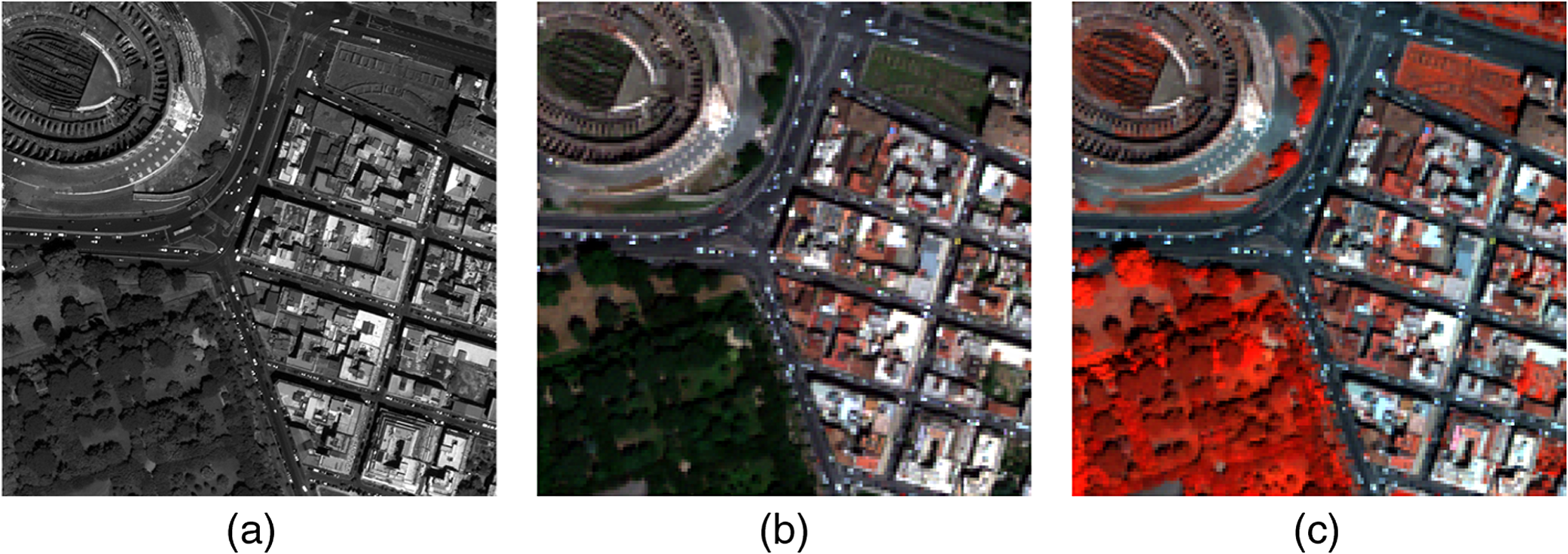 In an effort to evaluate the performance of our methods on lower resolution imagery, we tested our algorithm on the USGS EO-1 dataset scene of Victor, New York, shown in Fig. 9. The EO-1 multispectral dataset contains nine spectral bands with 30-m spatial resolution for the spectral image and 10-m resolution for the PAN band. Although the spatial resolution ratio between the PAN band and the multispectral bands is , we can still follow the similar pattern in Fig. 2 to calculate local difference factors. The resultant pan-sharpened image shown in Fig. 10 indicates that our algorithm also works well on lower resolution imagery. 3.2.Spectral AnalysisIn addition to visually observing the four complex scenes shown in the previous section, we also compared our results with several existing state-of-the-art pan-sharpening methods. These methods include Gram–Schmidt method,22 gMMSE method,18 and UNB sharpening method.13 These methods have been shown to produce high-quality fusion imagery, and brief descriptions of them can be found in the Sec. 1. The Gram–Schmidt method is integrated in ENVI; the authors of gMMSE have published a standalone package on their website, and the UNB method is distributed in the FuzeGo package that works on a trial license. Because these algorithms are available, a comparison is possible. The visual comparison of these algorithms can be made in Fig. 11 on a residential area from WorldView-2 image. It can be seen that all of these pan-sharpening approaches produce acceptable results. However, the edges in the Gram–Schmidt pan-sharpened image appear blurred. The gMMSE method produces better results, but the edges do not resemble the same level of sharpness in the PAN band. One possible reason is that both of these methods rely on a bicubic interpolation (or an alternative) as their basis for further processing, which leads to overly smooth edges if not correctly compensated. In comparison, both the UNB and our method produce images of very sharp contrast. Fig. 11Comparison of the various algorithms on the residential area scene. Panchromatic image and the RGB bands of the original images are shown in the upper left and upper middle. The marked pixels are used for spectra study, see Fig. 12 for details. The RGB bands of Gram-schmidt method, gMMSE, UNB and our method are shown in sequentially. 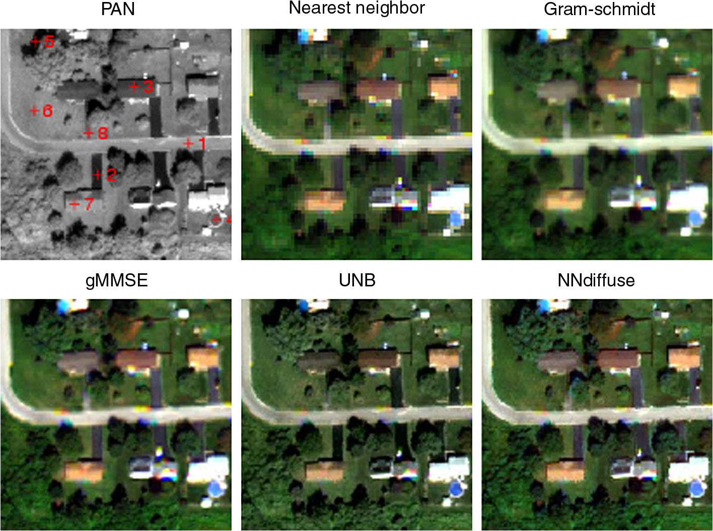 3.2.1.Pixel spectra evaluationThe spectral fidelity is another factor for evaluation of pan-sharpening algorithms. In this effort, we sample a number of signature pixels in relatively uniform areas to assess the spectral difference. These pixels are marked in the PAN image in Fig. 11. These pixels cover a large set of materials in the scene and are uniform around their neighborhood. We use the spectra from the original MSI image as ground truth for comparison with a reasonable assumption that the spectra around such uniform areas are most likely unchanged. The spectra resulting from the pan-sharpening algorithms are shown in Fig. 12, and the spectral difference expressed in spectral angle difference and Euclidean distance difference are shown in Table 3. It can be seen that both the gMMSE and our method can well preserve the spectra of these uniform pixels, whereas the spectra from Gram–Schmidt and UNB methods are very different from the truth. The majority of the error in our method comes from slight spectral bleeding from regions with weak edges. For example, the rooftop edge between pixel #7 and the grass is very weak in the PAN band; due to the fact that our algorithm is based on the difference distribution on the PAN, it allows a small amount of diffusion from the grass spectrum. The result is a slight increased digital count in the infrared band of the pan-sharpened pixel spectrum. In general, our method is seen to produce very small error by comparison. The spectral distortion by the UNB method can also be reflected by observing the color RGB images in Fig. 11; for example, the asphalt pavement is much darker in the UNB pan-sharpened image than in the original MSI image, and the color of the house rooftops is shifted. While the spectra in the visible regions are intact, the Gram–Schmidt method also suffers from severe spectral distortion in the near-infrared region. The Gram–Schmidt method assumes a statistical correlation between the PAN and each MSI band; however, the PAN band for the WorldView-2 imagery does not cover the NIR-2. The lack of correlation or even existence of anti-correlation results in the distortion of spectra in the infrared bands. One can also observe such spectral distortion in the NIR-2 from the images fused by both gMMSE and UNB; while our algorithm performs very well on most of the infrared regions, as shown in Fig. 12. In fact, most of the existing algorithms produce pan-sharpened images based on the band-to-band correlation, whereas our method treats the pixel spectra as the smallest element of operation which leads to relatively smaller spectral distortion even for the noncorrelated or low-correlated bands. In addition, our method operates locally and the results are always identical with no dependence on the size of the scene with given , , and . In comparison, most of the existing pan-sharpening algorithms rely, to a certain degree, on the global statistics of the scene, which may lead to somewhat different results depending on the scene content. Fig. 12Spectral comparison between the various approaches in the residential area scene. The spectra of the truth and produced from the various methods are shown. Figs. (a) to (h) correspond to the spectra of the pixels marked in PAN image of Fig. 11. 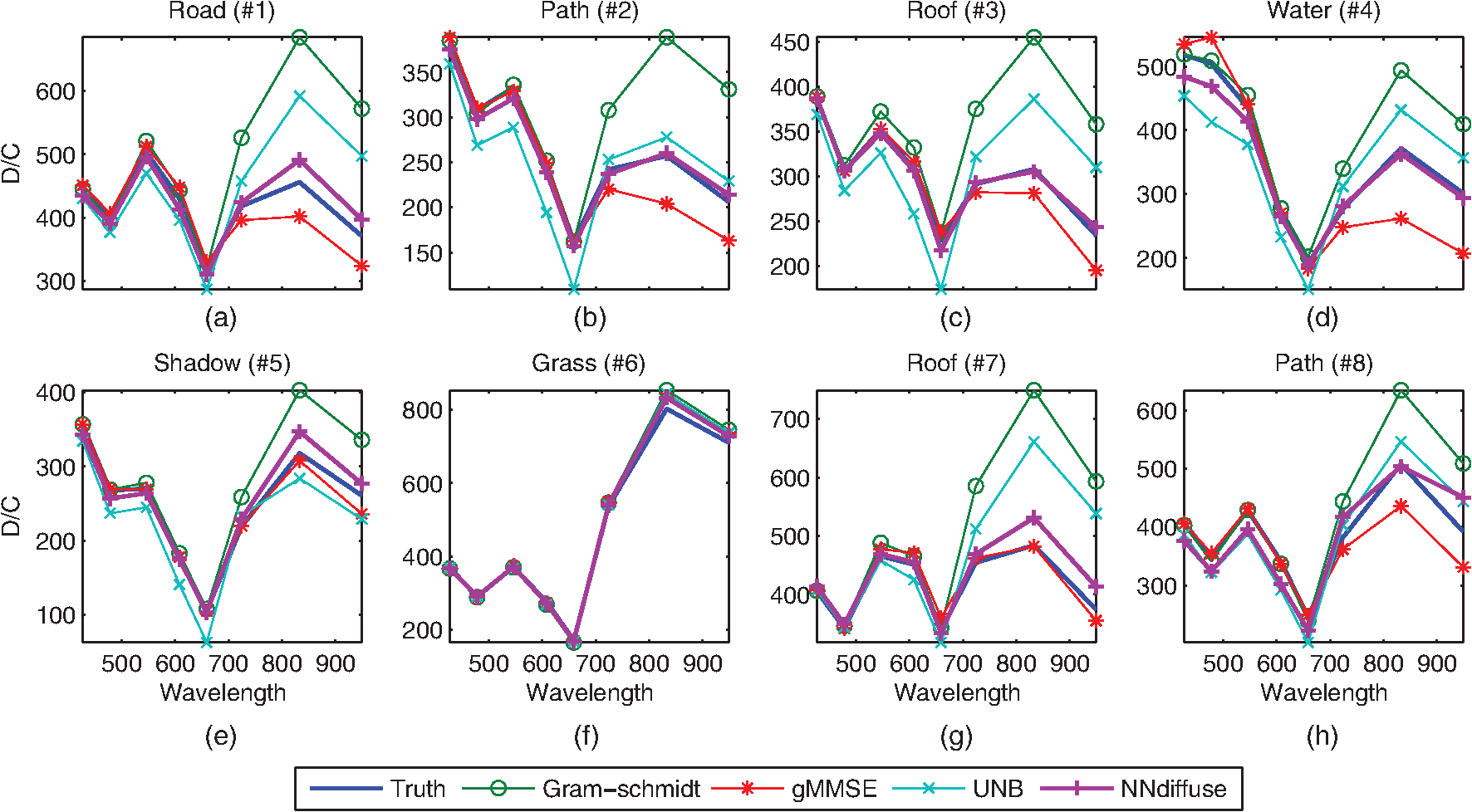 Table 3Spectral differences of sampled pixels in Fig. 12.
Note: Best (smallest) values are shown in bold. 3.2.2.Statistical comparisonAnother popular evaluation technique degrades the PAN and MSI images and uses the original MSI as the ground truth for comparison; the metrics include spectral angle mapper (SAM), spectral Euclidean distance (EUD), and erreur relative globale adimensionnelle de synthese ( ERGAS).32 SAM between two spectral vectors and is defined as where indicates the inner product. SAM basically computes a normalized correlation between two vectors. EUD is defined as and ERGAS is defined as where is the total number of bands, is the scale ratio, is the root-mean-square error between the ’th fused band and the reference band, and is the mean of the ’th band. ERGAS is a measure of global radiometric distortion of the fused images, and smaller ERGAS indicates better fusion results. We tested different algorithms on a degraded recycling site scene, and the metrics are shown in Table 4. The results are consistent with the above comparisons: our method and the gMMSE method preserve the overall spectra better than the Gram–Schmidt and the UNB methods. In addition to the global metric, cumulative error histograms of SAM and EUD are plotted in Fig. 13. While the global metric is capable of reflecting the fusion performance, the error histogram can better reflect the error distribution. Higher percentile in the lower error range indicates better fusion results. By observing the histogram, our method is able to produce much higher percentage of low SAM error (below 0.05) than the other methods; as for the EUD error, our method and gMMSE method have similar error distribution and perform better than the other two methods in the lower error range. The comparison reveals that our method is performing on the same level as the leading algorithms on statistical spectral fidelity with a slight advantage. It is worth mentioning that these evaluation metrics assume that the statistical signature and fusion performances are invariant to scale change; however, it has been suggested in recent literature18,24,33,34 that such an evaluation scheme is not practical especially for high-resolution data particularly in highly detailed urban areas where pan-sharpening is most needed. Thus, such comparison is only provided as one factor for evaluation.Table 4Comparison of the accuracy statistics for the degraded WorldView-2 recycling site scene.
Note: Best (smallest) values are shown in bold. Fig. 13Comparison of error histogram for the degraded WorldView-2 recycling site scene. (a) Error histogram w.r.t SAM, (b) Error histogram w.r.t to spectral EUD.  In this section, we performed a comprehensive comparison of different pan-sharpening algorithms through visual comparison, spectral comparison, and global statistics. Visual comparison indicates both UNB and our nearest-neighbor diffusion algorithm are more capable of enhancing the spatial sharpness than the other two methods; on the other hand, spectral accuracy is better reserved by both gMMSE and our algorithm through spectral and global statistics comparisons. Our method has shown to significantly suppress spectral angle distortion in comparison with the other methods. The comprehensive comparisons carried out in this section suggest that our nearest-neighbor diffusion-based approach can produce higher quality pan-sharpened spectral images than some state-of-the-art existing algorithms. 4.Discussion and Future WorkIn this article, we have shown our nearest-neighbor diffusion-based pan-sharpening method to have superior performance both in spatial/spectral quality and in computational time. The novelty of our approach lies in its per-spectra operation and the utilization of a diffusion model to solve the multispectral fusion problem. Our method operates locally and does not rely on global optimization and thus will produce identical results regardless of the scene size or scene contents. The parallel nature of our algorithm allows fast processing on multicore devices and achieves significant reduction of processing time. Our method relies on two external parameters: intensity smoothness factor and spatial smoothness factor that control the smoothness of the diffusion. Smaller values of restricts diffusion and thus produces sharper images but also introduces more noise, whereas larger values of will produce smoother contents with less noise. The proper choice of can be determined based on the application of the pan-sharpened image. is suggested to be tuned to a smaller value if it is for visual observation and inspection, while applications like classification and segmentation can use a larger to enhance strong structural features and to suppress noise artifacts. In addition, the scene contrast and complexity can also affect the choice of . Scenes with high contrast in PAN will need less diffusion sensitivity thus entail higher , and the same is true for complex scenes to reduce the influence of possible noise. In practice, is set to dynamically adjust to local similarity, as shown in Eq. (5), and is set to a value that will mostly resemble a bicubic interpolation kernel, which roughly gives . It is necessary to point out that the choice of and does not appear to have much impact on the visual results but will produce better numerical results compared with our previous findings.35 General readers may be interested in the execution speed of our algorithm, and we have implemented the algorithm in C/C++ to examine this. Our algorithm performs intensive localized operations. It is natural to extend our algorithm to work in parallel by taking advantage of the multicore architectures in modern day central processing unit (CPUs) and graphics processing unit (GPUs). We used OpenMP to accelerate our algorithm on the CPU. On the GPU, the algorithm is implemented using the CUDA architecture. Empirical analysis on an image set made up of a panchromatic image and a multispectral image showed an increase in processing speed of one order of magnitude on the OpenMP CPU and two orders of magnitude on the GPU. More analysis is required to fully characterize the computational speed-up potential of this algorithm. The proposed algorithm works well for urban scenes especially for objects with sharp edges observable in the PAN, but it may occasionally suffer from spectral bleeding at lower contrast PAN edges. In these cases, our algorithm may benefit by using IHS or UNB pan-sharpened images as a prior to produce difference factor , since these two methods have been known to preserve very high-spatial details. Furthermore, the difference factors can incorporate not only difference in the PAN, but also spectral difference from the MSI.36 In our method, we normalized the final spectra by stipulating pixel radiometric integrity (); however, other constraints can also be incorporated to obtain more accurate results, such as the spectra radiometric integrity calculated by In addition, our algorithm always assumes positive diffusion weights due to the exponent, and the implication is that only spectral summation, but no subtraction, is considered. In practice, spectral subtraction is needed to produce subpixel spectral accuracy; thus, adjusting diffusion weights to incorporate negative diffusion can also be designed to improve spectral and spatial accuracies. AcknowledgmentsThe authors are grateful to DigitalGlobe and USGS for generously providing the WorldView-2, GeoEye-1 and EO-1 imagery. The author (WS) would like to thank Dr. Sangmook Lee from Corning Incorporated for his useful suggestions in programming with CUDA and Dr. John R. Schott for providing valuable resources for algorithm improvement. This work is supported by Department of Energy Grant Number DE-NA0000444. ReferencesG. D. RobinsonH. N. GrossJ. R. Schott,
“Evaluation of two applications of spectral mixing models to image fusion,”
Remote Sens. Environ., 71
(3), 272
–281
(2000). http://dx.doi.org/10.1016/S0034-4257(99)00074-7 RSEEA7 0034-4257 Google Scholar
T.-M. Tuet al.,
“An adjustable pan-sharpening approach for ikonos/quickbird/geoeye-1/worldview-2 imagery,”
IEEE J. Sel. Top. Appl. Earth Obs. Remote Sens., 5
(1), 125
–134
(2012). http://dx.doi.org/10.1109/JSTARS.2011.2181827 1939-1404 Google Scholar
K. KotwalS. Chaudhuri,
“An optimization-based approach to fusion of hyperspectral images,”
IEEE J. Sel. Top. Appl. Earth Obs. Remote Sens., 5
(2), 501
–509
(2012). http://dx.doi.org/10.1109/JSTARS.2012.2187274 1939-1404 Google Scholar
A. Shiet al.,
“Multispectral and panchromatic image fusion based on improved bilateral filter,”
J. Appl. Remote Sens., 5
(1), 053542
(2011). http://dx.doi.org/10.1117/1.3616010 1931-3195 Google Scholar
A. MahyariM. Yazdi,
“Panchromatic and multispectral image fusion based on maximization of both spectral and spatial similarities,”
IEEE Trans. Geosci. Remote Sens., 49
(6), 1976
–1985
(2011). http://dx.doi.org/10.1109/TGRS.2010.2103944 IGRSD2 0196-2892 Google Scholar
K. KotwalS. Chaudhuri,
“Visualization of hyperspectral images using bilateral filtering,”
IEEE Trans. Geosci. Remote Sens., 48
(5), 2308
–2316
(2010). http://dx.doi.org/10.1109/TGRS.2009.2037950 IGRSD2 0196-2892 Google Scholar
J. LeeC. Lee,
“Fast and efficient panchromatic sharpening,”
IEEE Trans. Geosci. Remote Sens., 48
(1), 155
–163
(2010). http://dx.doi.org/10.1109/TGRS.2009.2028613 IGRSD2 0196-2892 Google Scholar
I. Amroet al.,
“A survey of classical methods and new trends in pansharpening of multispectral images,”
EURASIP J. Adv. Signal Process., 2011
(1), 1
–22
(2011). http://dx.doi.org/10.1186/1687-6180-2011-79 1687-6180 Google Scholar
Z. Wanget al.,
“A comparative analysis of image fusion methods,”
IEEE Trans. Geosci. Remote Sens., 43
(6), 1391
–1402
(2005). http://dx.doi.org/10.1109/TGRS.2005.846874 IGRSD2 0196-2892 Google Scholar
M. Gonzalez-Audicanaet al.,
“Comparison between mallat’s and the ‘à trous’ discrete wavelet transform based algorithms for the fusion of multispectral and panchromatic images,”
Int. J. Remote Sens., 26
(3), 595
–614
(2005). http://dx.doi.org/10.1080/01431160512331314056 IJSEDK 0143-1161 Google Scholar
V. Shettigara,
“A generalized component substitution technique for spatial enhancement of multispectral images using a higher resolution data set,”
Photogramm. Eng. Remote Sens., 58
(5), 561
–567
(1992). PGMEA9 0099-1112 Google Scholar
J. Schott, Remote Sensing: the Image Chain Approach, Oxford University Press, USA
(2007). Google Scholar
Y. Zhang,
“A new automatic approach for effectively fusing LANDSAT 7 as well as ikonos images,”
in 2002 IEEE International Geoscience and Remote Sensing Symposium, IGARSS’02,
2429
–2431
(2002). Google Scholar
D. Pradines,
“Improving spot images size and multispectral resolution,”
Proc. SPIE, 660 78
–102
(1986). http://dx.doi.org/10.1117/12.938572 PSISDG 0277-786X Google Scholar
J. C. Price,
“Combining panchromatic and multispectral imagery from dual resolution satellite instruments,”
Remote sens. Environ., 21
(2), 119
–128
(1987). http://dx.doi.org/10.1016/0034-4257(87)90049-6 RSEEA7 0034-4257 Google Scholar
B. Aiazziet al.,
“Context-driven fusion of high spatial and spectral resolution images based on oversampled multiresolution analysis,”
IEEE Trans. Geosci. Remote Sens., 40
(10), 2300
–2312
(2002). http://dx.doi.org/10.1109/TGRS.2002.803623 IGRSD2 0196-2892 Google Scholar
A. GarzelliF. Nencini,
“Interband structure modeling for pan-sharpening of very high-resolution multispectral images,”
Inform. Fusion, 6
(3), 213
–224
(2005). http://dx.doi.org/10.1016/j.inffus.2004.06.008 1566-2535 Google Scholar
A. GarzelliF. NenciniL. Capobianco,
“Optimal MMSE pan sharpening of very high resolution multispectral images,”
IEEE Trans. Geosci. Remote Sens., 46
(1), 228
–236
(2008). http://dx.doi.org/10.1109/TGRS.2007.907604 IGRSD2 0196-2892 Google Scholar
J. Nunezet al.,
“Multiresolution-based image fusion with additive wavelet decomposition,”
IEEE Trans. Geosci. Remote Sens., 37
(3), 1204
–1211
(1999). http://dx.doi.org/10.1109/36.763274 IGRSD2 0196-2892 Google Scholar
X. Otazuet al.,
“Introduction of sensor spectral response into image fusion methods. application to wavelet-based methods,”
IEEE Trans. Geosci. Remote Sens., 43
(10), 2376
–2385
(2005). http://dx.doi.org/10.1109/TGRS.2005.856106 IGRSD2 0196-2892 Google Scholar
J. R. Jensen, Remote Sensing of the Environment: An Earth Resource Perspective 2/e, Pearson Education, Delhi, India
(2009). Google Scholar
L. Alparoneet al.,
“Comparison of pansharpening algorithms: outcome of the 2006 GRS-S data-fusion contest,”
IEEE Trans. Geosci. Remote Sens., 45
(10), 3012
–3021
(2007). http://dx.doi.org/10.1109/TGRS.2007.904923 IGRSD2 0196-2892 Google Scholar
Y. ZhangR. Mishra,
“A review and comparison of commercially available pan-sharpening techniques for high resolution satellite image fusion,”
in 2012 IEEE International Geoscience and Remote Sensing Symposium (IGARSS),
182
–185
(2012). Google Scholar
A. Colorniet al.,
“Distributed optimization by ant colonies,”
in Proceedings of the first European conference on artificial life,
134
–142
(1991). Google Scholar
L. AshokD. W. Messinger,
“A spectral image clustering algorithm based on ant colony optimization,”
Proc. SPIE, 8390 83901P
(2012). http://dx.doi.org/10.1117/12.919082 PSISDG 0277-786X Google Scholar
P. PeronaJ. Malik,
“Scale-space and edge detection using anisotropic diffusion,”
IEEE Trans. Pattern Anal. Mach. Intell., 12
(7), 629
–639
(1990). http://dx.doi.org/10.1109/34.56205 ITPIDJ 0162-8828 Google Scholar
U.S. Geological Survey, “Sensors—advanced land imager (ali),”
(2011) http://eo1.usgs.gov/sensors/ali December ). 2011). Google Scholar
U.S. Geological Survey, “Sensors—hyperion,”
(2011) http://eo1.usgs.gov/sensors/hyperion December ). 2011). Google Scholar
Digital Globe, “Worldview-2 spacecraft data sheet—digitalglobe,”
http://www.digitalglobe.com/downloads/WorldView2DSWV2Web.pdf March ). Google Scholar
Digital Globe, “Geoeye-1 data sheet,”
http://www.digitalglobe.com/sites/default/files/DG_GeoEye1_DS.pdf June ). Google Scholar
L. Waldet al.,
“Fusion of satellite images of different spatial resolutions: assessing the quality of resulting images,”
Photogramm. Eng. Remote Sens., 63
(6), 691
–699
(1997). PGMEA9 0099-1112 Google Scholar
S. KlonusM. Ehlers,
“Performance of evaluation methods in image fusion,”
in 12th International Conference on, Information Fusion, 2009, FUSION ‘09,
1409
–1416
(2009). Google Scholar
Y. Kimet al.,
“Improved additive-wavelet image fusion,”
IEEE Geosci. Remote Sens. Lett., 8
(2), 263
–267
(2011). http://dx.doi.org/10.1109/LGRS.2010.2067192 IGRSBY 1545-598X Google Scholar
W. SunB. ChenD. W. Messinger,
“Pan-sharpening of spectral image with anisotropic diffusion for fine feature extraction using GPU,”
Proc. SPIE, 8743 87431H
(2013). http://dx.doi.org/10.1117/12.2015084 PSISDG 0277-786X Google Scholar
B. ChenA. VodacekN. Cahill,
“A novel adaptive scheme for evaluating spectral similarity in high-resolution urban scenes,”
IEEE J. Sel. Top. Appl. Earth Obs. Remote Sens., 6
(3), 1376
–1385
(2013). http://dx.doi.org/10.1109/JSTARS.2013.2254702 1939-1404 Google Scholar
BiographyWeihua Sun is a PhD student at the Center for Imaging Science at Rochester Institute of Technology (RIT). His research interests are imaging processing, machine learning, and algorithm development on multispectral and hyperspectral images. Currently, his work is focused on feature extraction from aerial images to aid scene development. He also has a MS and BS degrees in physics from Nanjing University, where his research area was design, simulation, and fabrication of optical metamaterials. Bin Chen received his BS degree in optical information science and the MS degree in optical engineering from Nanjing University of Science and Technology, Nanjing, China, in 2006 and 2008, respectively. He is currently pursuing the PhD degree in imaging science at Rochester Institute of Technology, Rochester, New York. His research interests include object recognition in high-resolution remote sensing images using hybrid algorithms and multisource data fusion. David W. Messinger received a bachelor’s degree in physics from Clarkson University and a PhD in physics from Rensselaer Polytechnic Institute. He is an associate research professor in the Chester F. Carlson Center for Imaging Science at the Rochester Institute of Technology, where he is the director of the digital imaging and remote sensing laboratory. His research focuses on remotely sensed spectral image exploitation using physics-based approaches and advanced mathematical techniques. |
||||||||||||||||||||||||||||||||||||||||||||||||||||||||||||||||||||||||||||||||||||||||||||||||||||||||||||||||||||||||||||||||||||||||||||||||||||||||||||||||||||||||