Polarization fields and wavefronts of two sheets for understanding polarization aberrations in optical imaging systems

José Sasián

doi:10.1117/1.OE.53.3.035102

17 March 2014 Polarization fields and wavefronts of two sheets for understanding polarization aberrations in optical imaging systems

José Sasián

Author Affiliations +

Optical Engineering, Vol. 53, Issue 3, 035102 (March 2014). https://doi.org/10.1117/1.OE.53.3.035102

Abstract

Polarization aberrations by highlighting the concepts of polarization aberration fields and of wavefronts of two sheets are explained. The fields have a vector character and are derived from the aberration function of plane symmetric systems. It is shown that in the presence of retardance, an incoming optical field is split into two fields and therefore one can speak of wavefronts of two sheets. Both concepts, polarization aberration fields and wavefronts of two sheets, ease the understanding of polarization aberrations.

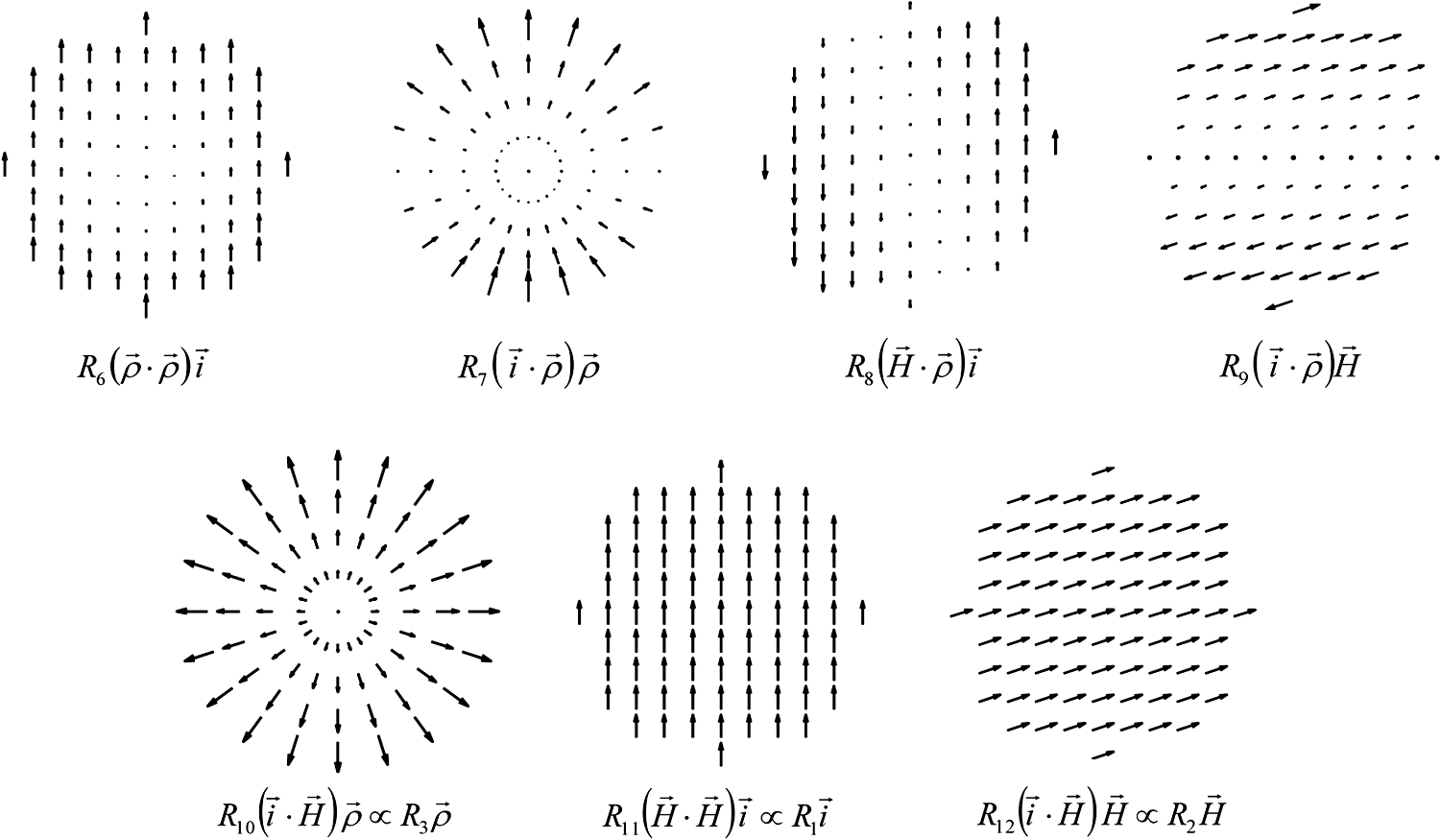
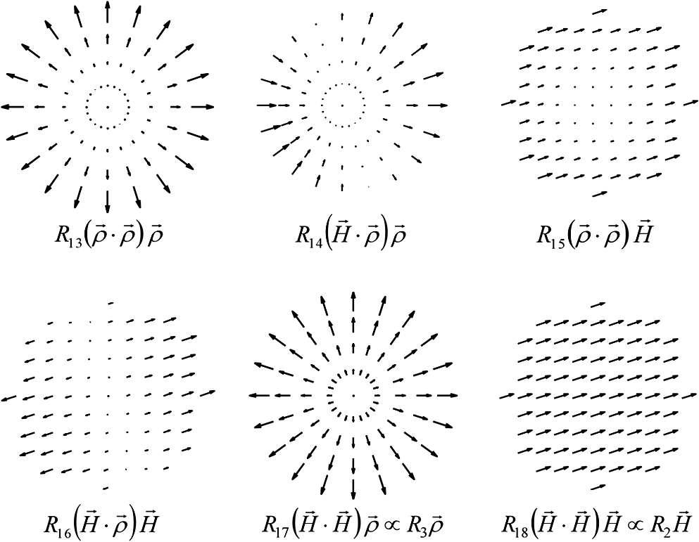
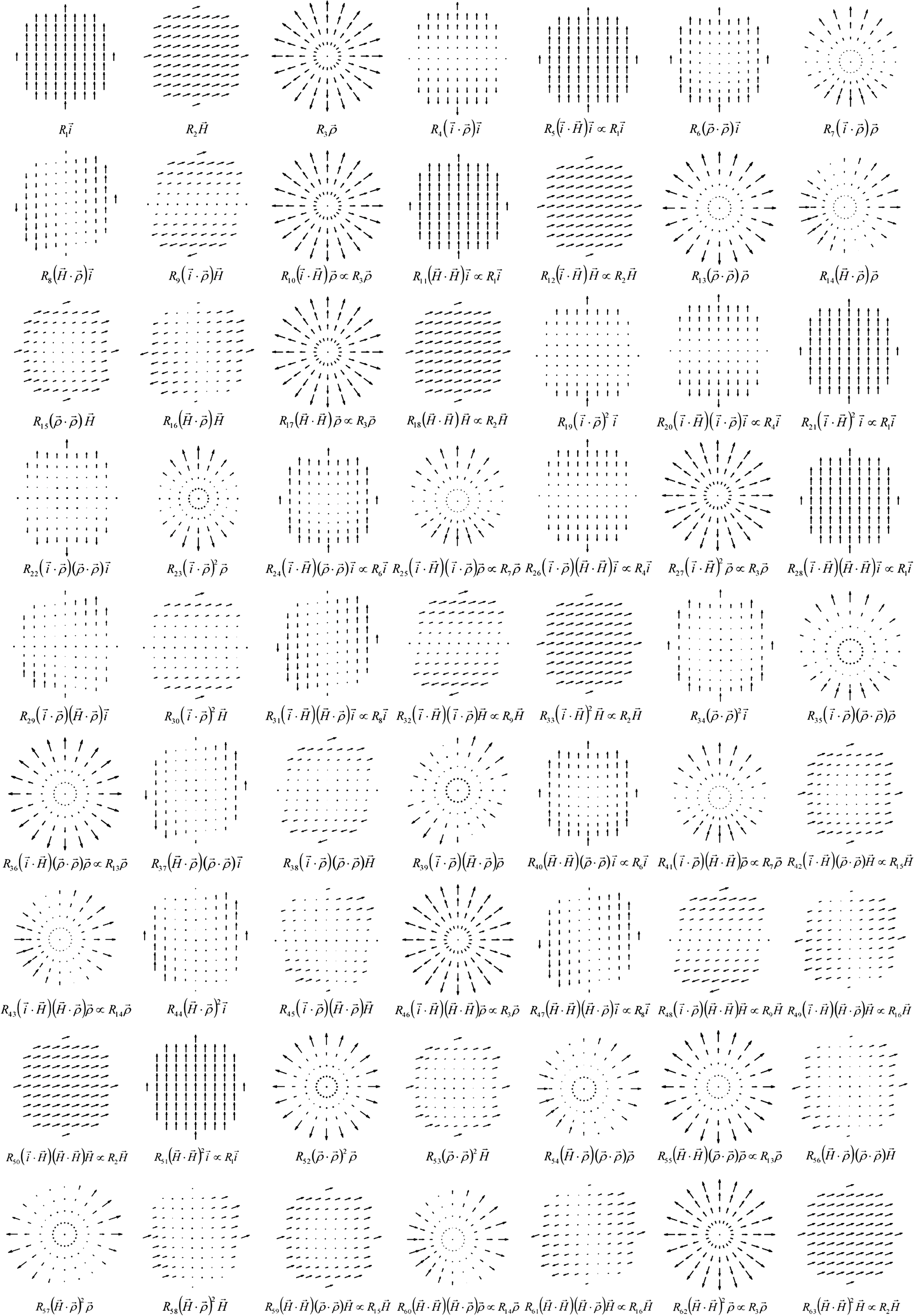
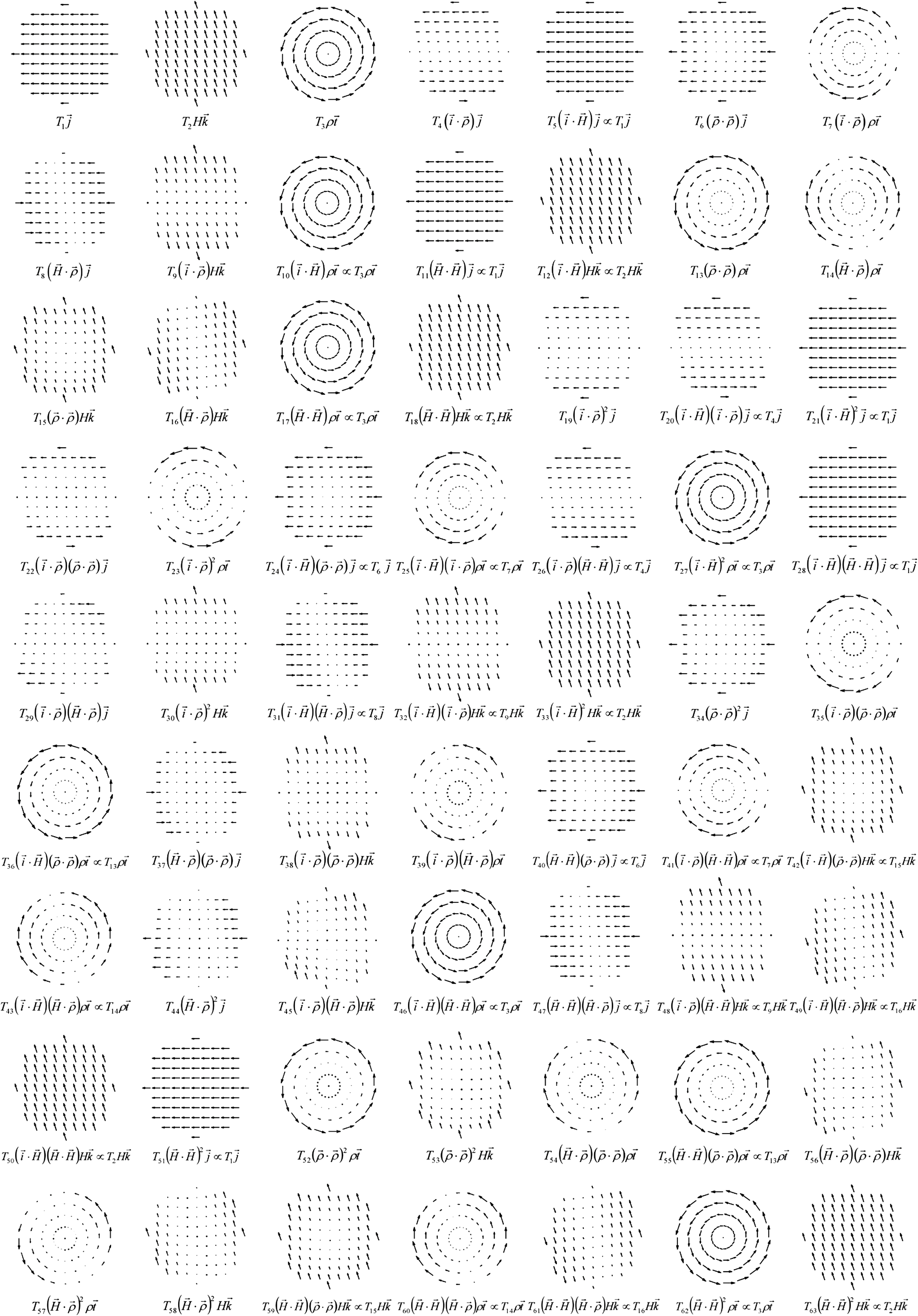
1. Introduction

The optical field originated from a point object changes as it interacts with an optical imaging system. The phase, amplitude, and polarization state of the optical field at the entrance pupil of the system can be adversely changed, that is aberrated, when it arrives at the exit pupil. The polarization effects of diattenuation and retardance are one reason for the optical field to change in an adverse manner for producing optimum imaging. Diattenuation refers to the difference in amplitude that the two polarization states may acquire upon refraction or reflection and retardance to the change in phase that those states can also acquire. Polarization issues in optical systems have been long known and some effects and their correction have been reported in the literature.¹^–⁸ The subject of polarization aberrations has been defined and studied previously⁹^,¹⁰ using a system’s Jones matrix, which depends on the field of view and the aperture of the system. This matrix is expanded, for example, in terms of the Pauli spin matrices to provide different terms that represent polarization aberrations.

This article provides an alternative way for understanding polarization aberrations by constructing a set of polarization fields.¹¹ These basic fields are useful not only for describing the optical field at the entrance pupil of the optical system but notably for describing the optical fields at the exit pupil as a superposition of basic fields. In this article, we provide equations and graphical displays for the first 63 polarization fields. We express the optical field at the entrance pupil plane of an axially symmetric optical system as

Eq. (1)

\vec{E} = \vec{A} (\vec{H}, \vec{ρ}) \exp [i \frac{2 π}{λ} Φ (\vec{H}, \vec{ρ})],

where the time dependence has been omitted,

\vec{A} (\vec{H}, \vec{ρ})

is the field amplitude in vector form, and

Φ (\vec{H}, \vec{ρ})

represents the optical phase; these depend on the field

\vec{H}

and aperture

\vec{ρ}

of the system.

We then show that in the presence of retardance the incoming optical field is split into two mutually orthogonal fields.

The surface of constant optical path is the wavefront and there exist two separated wavefronts, or a wavefront of two sheets, that produce two distinct images.

We develop and highlight the concepts of polarization fields and of wavefronts of two sheets for understanding polarization aberrations and imaging. These concepts ease the understanding of how the optical field propagates in an optical system and provide useful insight. Although the effects caused by diattenuation and retardance have been long known, there still exists a need for a clear theoretical foundation of the subject. This article aims at providing such a foundation while providing insight for optical engineering applications.

2. Construction of the Optical Fields

The first step is to define the optical field at the entrance pupil, and for this we construct the field amplitude $\vec{A} (\vec{H}, \vec{ρ})$ . Since we wish to construct fields that are smooth in their behavior with respect to the field and aperture of a system and that have symmetric properties, we use the aberration function of a plane symmetric system.¹² We establish the unit vector $\vec{i}$ in the field of view to define the direction of plane of symmetry. Since the aberration function is a scalar, it must depend on the dot products of the field vector $\vec{H}$ , the aperture vector $\vec{ρ}$ , and the symmetry vector $\vec{i}$ . This aberration function is written as

Eq. (2)

W (\vec{i}, \vec{H}, \vec{ρ}) = \sum_{k, m, n, p, q}^{\infty} W_{\underset{n, p, q}{\underset{2 m + n + q,}{2 k + n + p,}}} {(\vec{H} \cdot \vec{H})}^{k} {(\vec{ρ} \cdot \vec{ρ})}^{m} {(\vec{H} \cdot \vec{ρ})}^{n} {(\vec{i} \cdot \vec{H})}^{p} {(\vec{i} \cdot \vec{ρ})}^{q},

where

W_{2 k + n + p, 2 m + n + q, n, p, q}

is the coefficient of a particular aberration form defined by the integers

k

,

m

,

n

,

p

, and

q

. The lower indices in the coefficients indicate the algebraic powers of

H

,

ρ

,

\cos (ϕ)

,

\cos (χ)

, and

\cos (χ + ϕ)

in a given aberration term. The angle

χ

is between the vectors

\vec{i}

and

\vec{H}

, and the angle

ϕ

is between the vectors

\vec{H}

and

\vec{ρ}

, and the angle

χ + ϕ

is between the vectors

\vec{i}

and

\vec{ρ}

.

The fields, called here the ${\vec{R}}_{n}$ fields, must have a vector character; for constructing them we take the gradient of the aberration function for plane symmetric systems,

Eq. (3)

{\vec{R}}_{n} = {\vec{\nabla}}_{ρ} W (\vec{i}, \vec{H}, \vec{ρ}),

where for simplicity the lower index indicates a field number. We construct a complementary set of fields, called the

{\vec{T}}_{n}

fields, by rotating the

{\vec{R}}_{n}

fields by

π / 2

.

As shown in Fig. 1, we define the unit vector $\vec{r}$ parallel to $\vec{ρ}$ , the unit vector $\vec{t}$ perpendicular to $\vec{r}$ , the unit vector $\vec{h}$ parallel to $\vec{H}$ , the unit vector $\vec{k}$ perpendicular to $\vec{h}$ , and the unit vector $\vec{j}$ perpendicular to $\vec{i}$ . Vectors $\vec{i}$ and $\vec{j}$ are fixed and define the coordinate system. The vector $\vec{H} = H \vec{h}$ defines the field point, and the vector $\vec{ρ} = ρ \vec{r}$ defines the pupil point through which a given ray passes.

Fig. 1

Relation between unit vectors. Vectors $\vec{i}$ and $\vec{j}$ are fixed in orientation and define the coordinate system. The vectors $\vec{i}$ , $\vec{h}$ , and $\vec{r}$ are perpendicular to $\vec{j}$ , $\vec{k}$ , and $\vec{t}$ , respectively.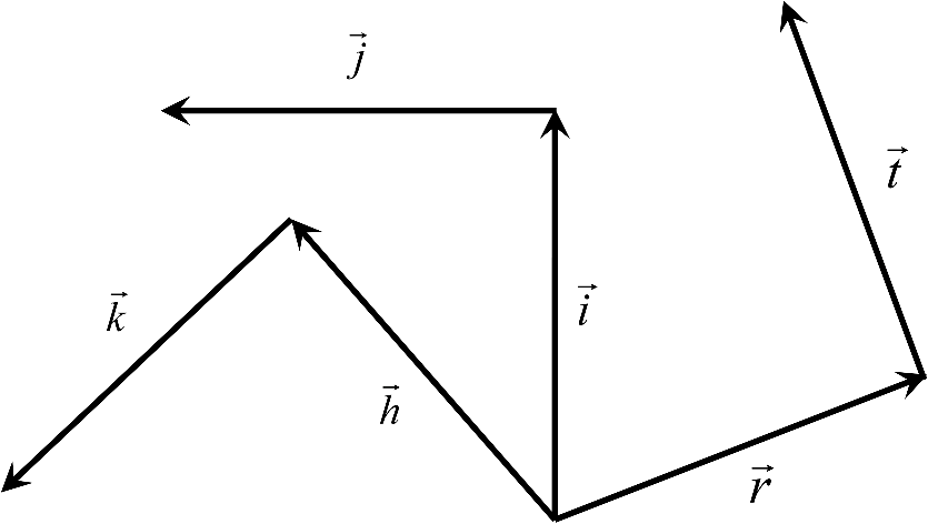

The first 63 ${\vec{R}}_{n}$ and ${\vec{T}}_{n}$ fields that result from taking the gradient of the aberration function for plane symmetric systems are given in Table 1. Piston terms have zero gradient and do not contribute to the fields. As a function of the symmetry, field, and aperture vectors, there are three fields of first order, fifteen fields of third order, and forty five fields of fifth order. The ${\vec{R}}_{n}$ and ${\vec{T}}_{n}$ fields are graphically shown in Appendices A and B, respectively; each field display is numbered and the functional dependence on the field, aperture, and coordinate vectors is also given next to each field. By construction, the ${\vec{R}}_{n}$ and ${\vec{T}}_{n}$ fields are orthogonal:

Eq. (4)

{\vec{R}}_{n} \cdot {\vec{T}}_{n} = 0,

Table 1

R→n and T→n fields.

Aberration term	${\vec{R}}_{n}$ field	${\vec{T}}_{n}$ field
First group
$W_{01001} (\vec{i} \cdot \vec{ρ})$	$R_{1} \vec{i}$	$T_{1} \vec{j}$
$W_{11100} (\vec{H} \cdot \vec{ρ})$	$R_{2} \vec{H}$	$T_{2} H \vec{k}$
$W_{02000} (\vec{ρ} \cdot \vec{ρ})$	$R_{3} \vec{ρ}$	$T_{3} ρ \vec{t}$
Second group
$W_{02002} {(\vec{i} \cdot \vec{ρ})}^{2}$	$R_{4} (\vec{i} \cdot \vec{ρ}) \vec{i}$	$T_{4} (\vec{i} \cdot \vec{ρ}) \vec{j}$
$W_{11011} (\vec{i} \cdot \vec{H}) (\vec{i} \cdot \vec{ρ})$	$R_{5} (\vec{i} \cdot \vec{H}) \vec{i}$	$T_{5} (\vec{i} \cdot \vec{H}) \vec{j}$
$W_{03001} (\vec{i} \cdot \vec{ρ}) (\vec{ρ} \cdot \vec{ρ})$	$R_{6} (\vec{ρ} \cdot \vec{ρ}) \vec{i}$	$T_{6} (\vec{ρ} \cdot \vec{ρ}) \vec{j}$
$W_{03001} (\vec{i} \cdot \vec{ρ}) (\vec{ρ} \cdot \vec{ρ})$	$R_{7} (\vec{i} \cdot \vec{ρ}) \vec{ρ}$	$T_{7} (\vec{i} \cdot \vec{ρ}) ρ \vec{t}$
$W_{12101} (\vec{i} \cdot \vec{ρ}) (\vec{H} \cdot \vec{ρ})$	$R_{8} (\vec{H} \cdot \vec{ρ}) \vec{i}$	$T_{8} (\vec{H} \cdot \vec{ρ}) \vec{j}$
$W_{12101} (\vec{i} \cdot \vec{ρ}) (\vec{H} \cdot \vec{ρ})$	$R_{9} (\vec{i} \cdot \vec{ρ}) \vec{H}$	$T_{9} (\vec{i} \cdot \vec{ρ}) H \vec{k}$
$W_{12010} (\vec{i} \cdot \vec{H}) (\vec{ρ} \cdot \vec{ρ})$	$R_{10} (\vec{i} \cdot \vec{H}) \vec{ρ}$	$T_{10} (\vec{i} \cdot \vec{H}) ρ \vec{t}$
$W_{21001} (\vec{i} \cdot \vec{ρ}) (\vec{H} \cdot \vec{H})$	$R_{11} (\vec{H} \cdot \vec{H}) \vec{i}$	$T_{11} (\vec{H} \cdot \vec{H}) \vec{j}$
$W_{21110} (\vec{i} \cdot \vec{H}) (\vec{H} \cdot \vec{ρ})$	$R_{12} (\vec{i} \cdot \vec{H}) \vec{H}$	$T_{12} (\vec{i} \cdot \vec{H}) H \vec{k}$
$W_{04000} {(\vec{ρ} \cdot \vec{ρ})}^{2}$	$R_{13} (\vec{ρ} \cdot \vec{ρ}) \vec{ρ}$	$T_{13} (\vec{ρ} \cdot \vec{ρ}) ρ \vec{t}$
$W_{13100} (\vec{H} \cdot \vec{ρ}) (\vec{ρ} \cdot \vec{ρ})$	$R_{14} (\vec{H} \cdot \vec{ρ}) \vec{ρ}$ $R_{15} (\vec{ρ} \cdot \vec{ρ}) \vec{H}$	$T_{14} (\vec{H} \cdot \vec{ρ}) ρ \vec{t}$ $T_{15} (\vec{ρ} \cdot \vec{ρ}) H \vec{k}$
$W_{22200} {(\vec{H} \cdot \vec{ρ})}^{2}$	$R_{16} (\vec{H} \cdot \vec{ρ}) \vec{H}$	$T_{16} (\vec{H} \cdot \vec{ρ}) H \vec{k}$
$W_{22000} (\vec{H} \cdot \vec{H}) (\vec{ρ} \cdot \vec{ρ})$	$R_{17} (\vec{H} \cdot \vec{H}) \vec{ρ}$	$T_{17} (\vec{H} \cdot \vec{H}) ρ \vec{t}$
$W_{31100} (\vec{H} \cdot \vec{H}) (\vec{H} \cdot \vec{ρ})$	$R_{18} (\vec{H} \cdot \vec{H}) \vec{H}$	$T_{18} (\vec{H} \cdot \vec{H}) H \vec{k}$
Third group
$W_{03003} {(\vec{i} \cdot \vec{ρ})}^{3}$	$R_{19} {(\vec{i} \cdot \vec{ρ})}^{2} \vec{i}$	$T_{19} {(\vec{i} \cdot \vec{ρ})}^{2} \vec{j}$
$W_{12012} (\vec{i} \cdot \vec{H}) {(\vec{i} \cdot \vec{ρ})}^{2}$	$R_{20} (\vec{i} \cdot \vec{H}) (\vec{i} \cdot \vec{ρ}) \vec{i}$	$T_{20} (\vec{i} \cdot \vec{H}) (\vec{i} \cdot \vec{ρ}) \vec{j}$
$W_{21021} {(\vec{i} \cdot \vec{H})}^{2} (\vec{i} \cdot \vec{ρ})$	$R_{21} {(\vec{i} \cdot \vec{H})}^{2} \vec{i}$	$T_{21} {(\vec{i} \cdot \vec{H})}^{2} \vec{j}$
$W_{04002} {(\vec{i} \cdot \vec{ρ})}^{2} (\vec{ρ} \cdot \vec{ρ})$	$R_{22} (\vec{i} \cdot \vec{ρ}) (\vec{ρ} \cdot \vec{ρ}) \vec{i}$ $R_{23} {(\vec{i} \cdot \vec{ρ})}^{2} \vec{ρ}$	$T_{22} (\vec{i} \cdot \vec{ρ}) (\vec{ρ} \cdot \vec{ρ}) \vec{j}$ $T_{23} {(\vec{i} \cdot \vec{ρ})}^{2} ρ \vec{t}$
$W_{13011} (\vec{i} \cdot \vec{H}) (\vec{i} \cdot \vec{ρ}) (\vec{ρ} \cdot \vec{ρ})$	$R_{24} (\vec{i} \cdot \vec{H}) (\vec{ρ} \cdot \vec{ρ}) \vec{i}$	$T_{24} (\vec{i} \cdot \vec{H}) (\vec{ρ} \cdot \vec{ρ}) \vec{j}$
	$R_{25} (\vec{i} \cdot \vec{H}) (\vec{i} \cdot \vec{ρ}) \vec{ρ}$	$T_{25} (\vec{i} \cdot \vec{H}) (\vec{i} \cdot \vec{ρ}) ρ \vec{t}$
$W_{22002} {(\vec{i} \cdot \vec{ρ})}^{2} (\vec{H} \cdot \vec{H})$	$R_{26} (\vec{i} \cdot \vec{ρ}) (\vec{H} \cdot \vec{H}) \vec{i}$	$T_{26} (\vec{i} \cdot \vec{ρ}) (\vec{H} \cdot \vec{H}) \vec{j}$
$W_{22020} {(\vec{i} \cdot \vec{H})}^{2} (\vec{ρ} \cdot \vec{ρ})$	$R_{27} {(\vec{i} \cdot \vec{H})}^{2} \vec{ρ}$	$T_{27} {(\vec{i} \cdot \vec{H})}^{2} ρ \vec{t}$
$W_{31011} (\vec{i} \cdot \vec{H}) (\vec{i} \cdot \vec{ρ}) (\vec{H} \cdot \vec{H})$	$R_{28} (\vec{i} \cdot \vec{H}) (\vec{H} \cdot \vec{H}) \vec{i}$	$T_{28} (\vec{i} \cdot \vec{H}) (\vec{H} \cdot \vec{H}) \vec{j}$
$W_{13102} {(\vec{i} \cdot \vec{ρ})}^{2} (\vec{H} \cdot \vec{ρ})$	$R_{29} (\vec{i} \cdot \vec{ρ}) (\vec{H} \cdot \vec{ρ}) \vec{i}$ $R_{30} {(\vec{i} \cdot \vec{ρ})}^{2} \vec{H}$	$T_{29} (\vec{i} \cdot \vec{ρ}) (\vec{H} \cdot \vec{ρ}) \vec{j}$ $T_{30} {(\vec{i} \cdot \vec{ρ})}^{2} H \vec{k}$
$W_{22111} (\vec{i} \cdot \vec{H}) (\vec{i} \cdot \vec{ρ}) (\vec{H} \cdot \vec{ρ})$	$R_{31} (\vec{i} \cdot \vec{H}) (\vec{H} \cdot \vec{ρ}) \vec{i}$ $R_{32} (\vec{i} \cdot \vec{H}) (\vec{i} \cdot \vec{ρ}) \vec{H}$	$T_{31} (\vec{i} \cdot \vec{H}) (\vec{H} \cdot \vec{ρ}) \vec{j}$ $T_{32} (\vec{i} \cdot \vec{H}) (\vec{i} \cdot \vec{ρ}) H \vec{k}$
$W_{31120} {(\vec{i} \cdot \vec{H})}^{2} (\vec{H} \cdot \vec{ρ})$	$R_{33} {(\vec{i} \cdot \vec{H})}^{2} \vec{H}$	$T_{33} {(\vec{i} \cdot \vec{H})}^{2} H \vec{k}$
$W_{05001} (\vec{i} \cdot \vec{ρ}) {(\vec{ρ} \cdot \vec{ρ})}^{2}$	$R_{34} {(\vec{ρ} \cdot \vec{ρ})}^{2} \vec{i}$ $R_{35} (\vec{i} \cdot \vec{ρ}) (\vec{ρ} \cdot \vec{ρ}) \vec{ρ}$	$T_{34} {(\vec{ρ} \cdot \vec{ρ})}^{2} \vec{j}$ $T_{35} (\vec{i} \cdot \vec{ρ}) (\vec{ρ} \cdot \vec{ρ}) ρ \vec{t}$
$W_{14010} (\vec{i} \cdot \vec{H}) {(\vec{ρ} \cdot \vec{ρ})}^{2}$	$R_{36} (\vec{i} \cdot \vec{H}) (\vec{ρ} \cdot \vec{ρ}) \vec{ρ}$	$T_{36} (\vec{i} \cdot \vec{H}) (\vec{ρ} \cdot \vec{ρ}) ρ \vec{t}$
$W_{14101} (\vec{i} \cdot \vec{ρ}) (\vec{H} \cdot \vec{ρ}) (\vec{ρ} \cdot \vec{ρ})$	$R_{37} (\vec{H} \cdot \vec{ρ}) (\vec{ρ} \cdot \vec{ρ}) \vec{i}$	$T_{37} (\vec{H} \cdot \vec{ρ}) (\vec{ρ} \cdot \vec{ρ}) \vec{j}$
	$R_{38} (\vec{i} \cdot \vec{ρ}) (\vec{ρ} \cdot \vec{ρ}) \vec{H}$	$T_{38} (\vec{i} \cdot \vec{ρ}) (\vec{ρ} \cdot \vec{ρ}) H \vec{k}$
	$R_{39} (\vec{i} \cdot \vec{ρ}) (\vec{H} \cdot \vec{ρ}) \vec{ρ}$	$T_{39} (\vec{i} \cdot \vec{ρ}) (\vec{H} \cdot \vec{ρ}) ρ \vec{t}$
$W_{23001} (\vec{i} \cdot \vec{ρ}) (\vec{H} \cdot \vec{H}) (\vec{ρ} \cdot \vec{ρ})$	$R_{40} (\vec{H} \cdot \vec{H}) (\vec{ρ} \cdot \vec{ρ}) \vec{i}$	$T_{40} (\vec{H} \cdot \vec{H}) (\vec{ρ} \cdot \vec{ρ}) \vec{j}$
	$R_{41} (\vec{i} \cdot \vec{ρ}) (\vec{H} \cdot \vec{H}) \vec{ρ}$	$T_{41} (\vec{i} \cdot \vec{ρ}) (\vec{H} \cdot \vec{H}) ρ \vec{t}$
$W_{23110} (\vec{i} \cdot \vec{H}) (\vec{H} \cdot \vec{ρ}) (\vec{ρ} \cdot \vec{ρ})$	$R_{42} (\vec{i} \cdot \vec{H}) (\vec{ρ} \cdot \vec{ρ}) \vec{H}$	$T_{42} (\vec{i} \cdot \vec{H}) (\vec{ρ} \cdot \vec{ρ}) H \vec{k}$
	$R_{43} (\vec{i} \cdot \vec{H}) (\vec{H} \cdot \vec{ρ}) \vec{ρ}$	$T_{43} (\vec{i} \cdot \vec{H}) (\vec{H} \cdot \vec{ρ}) ρ \vec{t}$
$W_{23201} (\vec{i} \cdot \vec{ρ}) {(\vec{H} \cdot \vec{ρ})}^{2}$	$R_{44} {(\vec{H} \cdot \vec{ρ})}^{2} \vec{i}$	$T_{44} {(\vec{H} \cdot \vec{ρ})}^{2} \vec{j}$
	$R_{45} (\vec{i} \cdot \vec{ρ}) (\vec{H} \cdot \vec{ρ}) \vec{H}$	$T_{45} (\vec{i} \cdot \vec{ρ}) (\vec{H} \cdot \vec{ρ}) H \vec{k}$
$W_{32010} (\vec{i} \cdot \vec{H}) (\vec{H} \cdot \vec{H}) (\vec{ρ} \cdot \vec{ρ})$	$R_{46} (\vec{i} \cdot \vec{H}) (\vec{H} \cdot \vec{H}) \vec{ρ}$	$T_{46} (\vec{i} \cdot \vec{H}) (\vec{H} \cdot \vec{H}) ρ \vec{t}$
$W_{32101} (\vec{i} \cdot \vec{ρ}) (\vec{H} \cdot \vec{H}) (\vec{H} \cdot \vec{ρ})$	$R_{47} (\vec{H} \cdot \vec{H}) (\vec{H} \cdot \vec{ρ}) \vec{i}$	$T_{47} (\vec{H} \cdot \vec{H}) (\vec{H} \cdot \vec{ρ}) \vec{j}$
	$R_{48} (\vec{i} \cdot \vec{ρ}) (\vec{H} \cdot \vec{H}) \vec{H}$	$T_{48} (\vec{i} \cdot \vec{ρ}) (\vec{H} \cdot \vec{H}) H \vec{k}$
$W_{32210} (\vec{i} \cdot \vec{H}) {(\vec{H} \cdot \vec{ρ})}^{2}$	$R_{49} (\vec{i} \cdot \vec{H}) (\vec{H} \cdot \vec{ρ}) \vec{H}$	$T_{49} (\vec{i} \cdot \vec{H}) (\vec{H} \cdot \vec{ρ}) H \vec{k}$
$W_{41110} (\vec{i} \cdot \vec{H}) (\vec{H} \cdot \vec{H}) (\vec{H} \cdot \vec{ρ})$	$R_{50} (\vec{i} \cdot \vec{H}) (\vec{H} \cdot \vec{H}) \vec{H}$	$T_{50} (\vec{i} \cdot \vec{H}) (\vec{H} \cdot \vec{H}) H \vec{k}$
$W_{41001} (\vec{i} \cdot \vec{ρ}) {(\vec{H} \cdot \vec{H})}^{2}$	$R_{51} {(\vec{H} \cdot \vec{H})}^{2} \vec{i}$	$T_{51} {(\vec{H} \cdot \vec{H})}^{2} \vec{j}$
$W_{06000} {(\vec{ρ} \cdot \vec{ρ})}^{3}$	$R_{52} {(\vec{ρ} \cdot \vec{ρ})}^{2} \vec{ρ}$	$T_{52} {(\vec{ρ} \cdot \vec{ρ})}^{2} ρ \vec{t}$
$W_{15100} (\vec{H} \cdot \vec{ρ}) {(\vec{ρ} \cdot \vec{ρ})}^{2}$	$R_{53} {(\vec{ρ} \cdot \vec{ρ})}^{2} \vec{H}$	$T_{53} {(\vec{ρ} \cdot \vec{ρ})}^{2} H \vec{k}$
	$R_{54} (\vec{H} \cdot \vec{ρ}) (\vec{ρ} \cdot \vec{ρ}) \vec{ρ}$	$T_{54} (\vec{H} \cdot \vec{ρ}) (\vec{ρ} \cdot \vec{ρ}) ρ \vec{t}$
$W_{24000} (\vec{H} \cdot \vec{H}) {(\vec{ρ} \cdot \vec{ρ})}^{2}$	$R_{55} (\vec{H} \cdot \vec{H}) (\vec{ρ} \cdot \vec{ρ}) \vec{ρ}$	$T_{55} (\vec{H} \cdot \vec{H}) (\vec{ρ} \cdot \vec{ρ}) ρ \vec{t}$
$W_{24200} {(\vec{H} \cdot \vec{ρ})}^{2} (\vec{ρ} \cdot \vec{ρ})$	$R_{56} (\vec{H} \cdot \vec{ρ}) (\vec{ρ} \cdot \vec{ρ}) \vec{H}$	$T_{56} (\vec{H} \cdot \vec{ρ}) (\vec{ρ} \cdot \vec{ρ}) H \vec{k}$
	$R_{57} {(\vec{H} \cdot \vec{ρ})}^{2} \vec{ρ}$	$T_{57} {(\vec{H} \cdot \vec{ρ})}^{2} ρ \vec{t}$
$W_{33300} {(\vec{H} \cdot \vec{ρ})}^{3}$	$R_{58} {(\vec{H} \cdot \vec{ρ})}^{2} \vec{H}$	$T_{58} {(\vec{H} \cdot \vec{ρ})}^{2} H \vec{k}$
$W_{33100} (\vec{H} \cdot \vec{H}) (\vec{H} \cdot \vec{ρ}) (\vec{ρ} \cdot \vec{ρ})$	$R_{59} (\vec{H} \cdot \vec{H}) (\vec{ρ} \cdot \vec{ρ}) \vec{H}$	$T_{59} (\vec{H} \cdot \vec{H}) (\vec{ρ} \cdot \vec{ρ}) H \vec{k}$
	$R_{60} (\vec{H} \cdot \vec{H}) (\vec{H} \cdot \vec{ρ}) \vec{ρ}$	$T_{60} (\vec{H} \cdot \vec{H}) (\vec{H} \cdot \vec{ρ}) ρ \vec{t}$
$W_{42200} (\vec{H} \cdot \vec{H}) {(\vec{H} \cdot \vec{ρ})}^{2}$	$R_{61} (\vec{H} \cdot \vec{H}) (\vec{H} \cdot \vec{ρ}) \vec{H}$	$T_{61} (\vec{H} \cdot \vec{H}) (\vec{H} \cdot \vec{ρ}) H \vec{k}$
$W_{42000} {(\vec{H} \cdot \vec{H})}^{2} (\vec{ρ} \cdot \vec{ρ})$	$R_{62} {(\vec{H} \cdot \vec{H})}^{2} \vec{ρ}$	$T_{62} {(\vec{H} \cdot \vec{H})}^{2} ρ \vec{t}$
$W_{51100} {(\vec{H} \cdot \vec{H})}^{2} (\vec{H} \cdot \vec{ρ})$	$R_{63} {(\vec{H} \cdot \vec{H})}^{2} \vec{H}$	$T_{63} {(\vec{H} \cdot \vec{H})}^{2} H \vec{k}$

A different route to obtain the ${\vec{T}}_{n}$ fields is as follows.¹³ The components of ${\vec{R}}_{n}$ are on the pupil plane. Let the unit vectors $\vec{x}$ , $\vec{y}$ , and $\vec{z}$ define a Cartesian coordinate system with $\vec{z}$ parallel to the optical axis. Then, we can express the ${\vec{T}}_{n}$ fields as

Eq. (5)

{\vec{T}}_{n} = curl [W (\vec{i}, \vec{H}, \vec{ρ}) \vec{z}] = \vec{x} \frac{\partial W (\vec{i}, \vec{H}, \vec{ρ})}{\partial y} - \vec{y} \frac{\partial W (\vec{i}, \vec{H}, \vec{ρ})}{\partial x} .

Since

Eq. (6)

{\vec{R}}_{n} = \vec{\nabla} W (\vec{i}, \vec{H}, \vec{ρ}) = \vec{x} \frac{\partial W (\vec{i}, \vec{H}, \vec{ρ})}{\partial x} + \vec{y} \frac{\partial W (\vec{i}, \vec{H}, \vec{ρ})}{\partial y} .

We have that

{\vec{R}}_{n} \cdot {\vec{T}}_{n} = 0

as

{\vec{T}}_{n}

results by rotation of

{\vec{R}}_{n}

by

π / 2

; this is

{\vec{T}}_{n} = \vec{j} {\vec{R}}_{n}

.

Furthermore, since the curl of ${\vec{R}}_{n}$ is zero then the ${\vec{R}}_{n}$ fields are irrotational; and since the divergence of ${\vec{T}}_{n}$ is zero then the ${\vec{T}}_{n}$ fields are solenoidal. A given vector field that is continuous as well as its derivatives can be resolved into an irrotational part and a solenoidal part. Thus, the ${\vec{R}}_{n}$ and ${\vec{T}}_{n}$ are an adequate basis to express the amplitude $\vec{A}$ of an optical field. For completeness purposes, we have presented the first 63 ${\vec{R}}_{n}$ and ${\vec{T}}_{n}$ fields. In practice, however, one would be mostly concerned with the low-order fields; high-order fields represent higher-order amplitude polarization aberrations.

3. Optical Field Changes of Second Order

In this section, we determine the optical field changes to second order of approximation as a function of the field and aperture of an optical system. These changes relate to the field amplitude and to the field phase. Assume an optical system where the stop aperture is located at the center of curvature of a spherical surface. Therefore, the entrance and exit pupils coincide with the stop location. At the entrance pupil, we have the optical field $\vec{E}$

Eq. (7)

\vec{E} = \vec{A} (\vec{H}, \vec{ρ}) \exp [i \frac{2 π}{λ} Φ (\vec{H}, \vec{ρ})],

where

\vec{A} (\vec{H}, \vec{ρ})

, or simply

\vec{A}

, is the field amplitude and

Φ (\vec{H}, \vec{ρ})

is the optical phase, which depends on the field and aperture of the system.

When light is refracted by the surface the polarization state may be changed. For the $s$ polarization state, the surface may change the field amplitude by the factor $t_{s}$ and introduce a phase change $(2 π / λ) δ A^{2} (\vec{ρ} \cdot \vec{ρ})$ . For the $p$ polarization state, the surface may change the field amplitude by the factor $t_{p}$ and introduce a phase change $(2 π / λ) (δ + Δ δ) A^{2} (\vec{ρ} \cdot \vec{ρ})$ . The coefficients $δ$ and $Δ δ$ describe phase changes or retardance, and the parameter $A = n i$ where $i$ is the first-order marginal ray angle (slope) of incidence on the surface. According to the Fresnel equations, an uncoated refracting surface does not contribute retardance; however, if the surface has an optical coating then retardance takes place. Retardance is also introduced from light reflection on a metal. The retardance is usually a fraction of a wavelength and to be significant it requires large angles of incidence. In high-numerical-aperture, multilens systems, the cumulative effects of retardance need to be taken into account. The coefficients $δ$ and $Δ δ$ can analytically be calculated for simple structures but they can be obtained from phase changes data provided by an optical thin films program.

From the Fresnel equations, the amplitude coefficients $t_{s}$ and $t_{p}$ upon light refraction can be derived and to second order of approximation these are

Eq. (8)

t_{s} = T + T t A^{2} (\vec{ρ} \cdot \vec{ρ}),

Eq. (9)

t_{p} = T + T (t + Δ t) A^{2} (\vec{ρ} \cdot \vec{ρ}),

where

Eq. (10)

T = \frac{2 n}{n^{'} + n},

Eq. (11)

t = - \frac{1}{2} (\frac{n^{'} - n}{n^{2} n^{'}}),

Eq. (12)

Δ t = \frac{1}{2} {(\frac{n^{'} - n}{n n^{'}})}^{2} .

The optical field is described at the entrance pupil plane located at the surface’s center of curvature, and to second order of approximation, the unit vector $\vec{r}$ is in the plane of incidence of a ray specified by $\vec{H}$ and $\vec{ρ}$ , and the unit vector $\vec{t}$ is perpendicular to the plane of incidence of the ray.

After light refraction the field ${\vec{E}}^{'}$ at the exit pupil can be written as if both amplitude and phase changes occur simultaneously

Eq. (13)

{\vec{E}}^{'} = \exp [i \frac{2 π}{λ} δ A^{2} (\vec{ρ} \cdot \vec{ρ})] {t_{s} (\vec{E} \cdot \vec{t}) \vec{t} + \exp [i \frac{2 π}{λ} Δ δ A^{2} (\vec{ρ} \cdot \vec{ρ})] t_{p} (\vec{E} \cdot \vec{r}) \vec{r}},

or as if amplitude and phase changes occur sequentially. For simplicity, we take the later route.

When there is no retardance $Δ δ = 0$ between the two polarization states, the optical field ${\vec{E}}^{'}$ can be written as

Eq. (14)

{\vec{E}}^{'} = \exp [i \frac{2 π}{λ} δ A^{2} (\vec{ρ} \cdot \vec{ρ})] [t_{s} (\vec{E} \cdot \vec{t}) \vec{t} + t_{p} (\vec{E} \cdot \vec{r}) \vec{r}] = \exp [i \frac{2 π}{λ} δ A^{2} (\vec{ρ} \cdot \vec{ρ})] {[T + T t A^{2} (\vec{ρ} \cdot \vec{ρ})] (\vec{E} \cdot \vec{t}) \vec{t} + [T + T (t + Δ t) A^{2} (\vec{ρ} \cdot \vec{ρ})] (\vec{E} \cdot \vec{r}) \vec{r}} = \exp [i \frac{2 π}{λ} δ A^{2} (\vec{ρ} \cdot \vec{ρ})] [T \vec{E} + T t A^{2} (\vec{ρ} \cdot \vec{ρ}) \vec{E} + T Δ t A^{2} (\vec{E} \cdot \vec{ρ}) \vec{ρ}] .

When the retardance $Δ δ$ is introduced the optical field ${\vec{E}}^{*}$ becomes

Eq. (15)

{\vec{E}}^{*} = \exp {i \frac{2 π}{λ} [\frac{1}{2} Δ δ A^{2} (\vec{ρ} \cdot \vec{ρ})]} \times {\begin{cases} ({\vec{E}}^{'} \cdot \vec{t}) \vec{t} \exp [- i \frac{2 π}{λ} \frac{1}{2} Δ δ A^{2} (\vec{ρ} \cdot \vec{ρ})] + \\ ({\vec{E}}^{'} \cdot \vec{r}) \vec{r} \exp [i \frac{2 π}{λ} \frac{1}{2} Δ δ A^{2} (\vec{ρ} \cdot \vec{ρ})] \end{cases}} .

We define the unit vector $\vec{a}$ parallel to ${\vec{E}}^{'}$ and the unit vector $\vec{b}$ perpendicular to ${\vec{E}}^{'}$ . Then, we write ${\vec{E}}^{'} = | {\vec{E}}^{'} | \vec{a}$ and define a field ${\vec{E}}^{' ⊥} = | {\vec{E}}^{'} | \vec{b}$ perpendicular to the field ${\vec{E}}^{'}$ .

The unit vectors $\vec{r}$ and $\vec{t}$ can be decomposed in a component parallel to $\vec{a}$ and a component parallel to $\vec{b}$ , where we have $| \vec{a} | = 1$ , $| \vec{b} | = 1$ , and $\vec{a} \cdot \vec{b} = 0$ . The decomposition is

Eq. (16)

\vec{r} = (\vec{a} \cdot \vec{r}) \vec{a} + (\vec{b} \cdot \vec{r}) \vec{b} \vec{t} = (\vec{a} \cdot \vec{t}) \vec{a} + (\vec{b} \cdot \vec{t}) \vec{b} .

We also can write the relationships

Eq. (17)

({\vec{E}}^{'} \cdot \vec{r}) \vec{r} = {(\vec{a} \cdot \vec{r})}^{2} {\vec{E}}^{'} + (\vec{a} \cdot \vec{r}) (\vec{b} \cdot \vec{r}) {\vec{E}}^{' ⊥} ({\vec{E}}^{'} \cdot \vec{t}) \vec{t} = {(\vec{a} \cdot \vec{t})}^{2} {\vec{E}}^{'} + (\vec{a} \cdot \vec{t}) (\vec{b} \cdot \vec{t}) {\vec{E}}^{' ⊥} .

The optical field at the exit pupil then becomes

Eq. (18)

{\vec{E}}^{*} = \exp {i \frac{2 π}{λ} [\frac{1}{2} Δ δ A^{2} (\vec{ρ} \cdot \vec{ρ})]} \times {\begin{cases} [{(\vec{a} \cdot \vec{t})}^{2} {\vec{E}}^{'} + (\vec{a} \cdot \vec{t}) (\vec{b} \cdot \vec{t}) {\vec{E}}^{' ⊥}] \exp [- i \frac{2 π}{λ} \frac{1}{2} Δ δ A^{2} (\vec{ρ} \cdot \vec{ρ})] + \\ [{(\vec{a} \cdot \vec{r})}^{2} {\vec{E}}^{'} + (\vec{a} \cdot \vec{r}) (\vec{b} \cdot \vec{r}) {\vec{E}}^{' ⊥}] \exp [i \frac{2 π}{λ} \frac{1}{2} Δ δ A^{2} (\vec{ρ} \cdot \vec{ρ})] \end{cases}} .

The field ${\vec{E}}^{*}$ can be separated into a component ${\vec{E}}^{o}$ parallel and a component ${\vec{E}}^{e}$ perpendicular to the field ${\vec{E}}^{'}$ . These field components ${\vec{E}}^{o}$ and ${\vec{E}}^{e}$ can be written (see Appendix C) as

Eq. (19)

{\vec{E}}^{o} = {\vec{E}}^{'} \exp {i \frac{2 π}{λ} [\frac{1}{2} Δ δ A^{2} (\vec{ρ} \cdot \vec{ρ})]} \sqrt{(\cos^{2} {\frac{2 π}{λ} \frac{1}{2} [Δ δ A^{2} (\vec{ρ} \cdot \vec{ρ})]} + \sin^{2} {\frac{2 π}{λ} \frac{1}{2} [Δ δ A^{2} (\vec{ρ} \cdot \vec{ρ})]} {[{(\vec{a} \cdot \vec{r})}^{2} - {(\vec{a} \cdot \vec{t})}^{2}]}^{2})} \exp [i \times arct (Tan {\frac{2 π}{λ} \frac{1}{2} [Δ δ A^{2} (\vec{ρ} \cdot \vec{ρ})]} [{(\vec{a} \cdot \vec{r})}^{2} - {(\vec{a} \cdot \vec{t})}^{2}])] ≅ {\vec{E}}^{'} \exp {i \frac{2 π}{λ} [Δ δ A^{2} {(\vec{a} \cdot \vec{ρ})}^{2}]}

and

Eq. (20)

{\vec{E}}^{e} = {\vec{E}}^{' ⊥} \exp {i \frac{2 π}{λ} [\frac{1}{2} Δ δ A^{2} (\vec{ρ} \cdot \vec{ρ})] + i \frac{π}{2}} [2 (\vec{a} \cdot \vec{r}) (\vec{b} \cdot \vec{r})] [\sin \frac{2 π}{λ} \frac{1}{2} Δ δ A^{2} (\vec{ρ} \cdot \vec{ρ})] ≅ {\vec{E}}^{' ⊥} \exp {i \frac{2 π}{λ} [\frac{1}{2} Δ δ A^{2} (\vec{ρ} \cdot \vec{ρ})] + i \frac{π}{2}} \times [\frac{2 π}{λ} Δ δ A^{2} (\vec{a} \cdot \vec{ρ}) (\vec{b} \cdot \vec{ρ})] .

We note that ${| {\vec{E}}^{o} |}^{2} + {| {\vec{E}}^{e} |}^{2} = {| {\vec{E}}^{'} |}^{2}$ and thus the energy in the ${\vec{E}}^{'}$ field is conserved and shared by the ${\vec{E}}^{o}$ and ${\vec{E}}^{e}$ fields.

The superscripts $o$ and $e$ are used to avoid confusion with the usage of parallel and perpendicular as they often refer to the plane of light incidence.

In this decomposition, each field component, ${\vec{E}}^{o}$ and ${\vec{E}}^{e}$ , has amplitude and phase and is perpendicular to the other over the entire pupil. Thus, the incoming optical field is split into two fields. Furthermore, for a given optical path length OPL from an object point, a wavefront can be defined for the ${\vec{E}}^{o}$ field. Similarly, for the same OPL a distinct and separated wavefront can be defined for the ${\vec{E}}^{e}$ field. Therefore, in the presence of retardance, we can speak of the concept of a wavefront of two sheets, one sheet belonging to the ${\vec{E}}^{o}$ field component, the other sheet belonging to the ${\vec{E}}^{e}$ field component. Given the wavefront of two sheets then two distinct images of the source point can be expected. Retardance, and therefore wavefront splitting, can be introduced by a thin film coating on a lens, by reflection on metal, or by a birefringent material. For example, by placing a $z$ -cut, uniaxial crystal in an optical system with its optical axis aligned with the system’s optical axis, one can introduce retardance due to the crystal birefringence.

4. Optical Field upon Stop Shifting

Now, we consider the optical field when the aperture stop is not located at the center of curvature of the spherical surface. For this we perform stop shifting, which is achieved by replacing in the fields ${\vec{E}}^{o}$ and ${\vec{E}}^{e}$ the aperture vector $\vec{ρ}$ with the shift vector ${\vec{ρ}}_{shift} = \vec{ρ} + (\bar{A} / A) \vec{H}$ and by term expansion.¹¹ The factor $\bar{A} = n \bar{i}$ where $\bar{i}$ is the first-order chief ray angle of incidence on the surface, and the factor $A = n i$ where $i$ is the first-order marginal angle of incidence. We only retain second-order terms as a function of the field vector $\vec{H}$ and the aperture vector $\vec{ρ}$ .

By substitution of the shift vector ${\vec{ρ}}_{shift}$ in ${\vec{E}}^{o}$ the field is obtained for a general stop location

Eq. (21)

{\vec{E}}^{o} (\vec{H}, \vec{ρ}) = T \exp {i \frac{2 π}{λ} δ [A^{2} (\vec{ρ} \cdot \vec{ρ}) + 2 \bar{A} A (\vec{H} \cdot \vec{ρ}) + {\bar{A}}^{2} (\vec{H} \cdot \vec{H})]} (\begin{array}{l} \vec{E} + t [A^{2} (\vec{ρ} \cdot \vec{ρ}) + 2 \bar{A} A (\vec{H} \cdot \vec{ρ}) + {\bar{A}}^{2} (\vec{H} \cdot \vec{H})] \vec{E} + \\ Δ t {[A^{2} (\vec{E} \cdot \vec{ρ}) \vec{ρ} + \bar{A} A (\vec{E} \cdot \vec{H}) \vec{ρ}] + [\bar{A} A (\vec{E} \cdot \vec{ρ}) \vec{H} + {\bar{A}}^{2} (\vec{E} \cdot \vec{H}) \vec{H}]} \end{array}) \exp (i \frac{2 π}{λ} {Δ δ [A^{2} {(\vec{a} \cdot \vec{ρ})}^{2} + 2 \bar{A} A (\vec{a} \cdot \vec{ρ}) (\vec{a} \cdot \vec{H}) + {\bar{A}}^{2} {(\vec{a} \cdot \vec{H})}^{2}]}) .

Similarly, for the ${\vec{E}}^{e}$ field component after neglecting fourth-order terms we can write

Eq. (22)

{\vec{E}}^{e} (\vec{H}, \vec{ρ}) = T \exp (i \frac{2 π}{λ} {(δ + \frac{1}{2} Δ δ) [A^{2} (\vec{ρ} \cdot \vec{ρ}) + 2 \bar{A} A (\vec{H} \cdot \vec{ρ}) + {\bar{A}}^{2} (\vec{H} \cdot \vec{H}) + \frac{λ}{4}]}) {\vec{E}}^{⊥} {\frac{2 π}{λ} Δ δ [\begin{array}{l} A (\vec{a} \cdot \vec{ρ}) (\vec{b} \cdot \vec{ρ}) + \bar{A} A (\vec{a} \cdot \vec{H}) (\vec{b} \cdot \vec{ρ}) + \\ A \bar{A} (\vec{a} \cdot \vec{ρ}) (\vec{b} \cdot \vec{H}) + {\bar{A}}^{2} (\vec{a} \cdot \vec{H}) (\vec{b} \cdot \vec{H}) \end{array}]},

where

{\vec{E}}^{⊥}

is the optical field

\vec{E}

rotated 90 deg. In both of these expressions, the field

\vec{E}

is at the entrance pupil after stop shifting. The field

\vec{E}

is either already known or is obtained by substitution of the shift

{\vec{ρ}}_{shift}

vector in the field at the plane of the surface center of curvature.

5. Polarization Aberration Coefficients

We now determine the coefficients that define the optical field for an optical system of several surfaces. We assume that to second order the individual surface coefficients add to form the coefficients for the entire optical system. The transmission from two surfaces is the product of the individual surface transmissions. However, when the amplitude factors have zero- and second-order terms, the second-order terms of the product are the sums of the second-order terms of the factors (weighted by the zero-order terms). Regarding phase, it follows from the fact that optical paths add, that we can add second-order phase terms. However, we neglect some extrinsic¹⁴ second-order terms that might be present due to the interaction between second-order terms due to light refraction and second-order terms due to polarization retardance. These extrinsic terms depend on the product of the gradient of second-order aberrations. Since second-order effects from retardance are small then the extrinsic contributions are expected to be comparatively negligible. Effectively, phase contributions due to pure refraction or reflection are accurately accounted by the first-order ray trace. However, when the phase is changed due to polarization retardance, then the standard first-order ray trace based on the surface optical powers will not fully account for first-order ray paths. There will be a small error which would be accounted for with extrinsic terms. One way to avoid first-order errors is to include the second-order phase contributions, optical power, from retardance in the first-order ray trace.

Table 2 presents a summary of second-order polarization aberration coefficients for a system of $q$ surfaces. These coefficients are the sums of individual surface coefficients for amplitude and phase terms. Their calculation requires the ray tracing of a marginal and a chief first-order (paraxial) rays. The factor $\bar{A} = n \bar{i}$ is the first-order chief ray refraction invariant, and the factor $A = n i$ is the first-order marginal ray refraction invariant. Those rays have paraxial angles (slopes) of incidence $\bar{i}$ and $i$ at a given system surface. Coefficients similar to the presented in Table 2 have been previously introduced by Chipman.¹⁵

Table 2

Polarization aberration coefficients for a system of q surfaces.

$P_{1} = T_{q} \sum_{j = 1}^{q} {(t A^{2})}_{j}$	$δ_{1} = \sum_{j = 1}^{q} {(δ A^{2})}_{j}$
$P_{2} = 2 T_{q} \sum_{j = 1}^{q} {(t A \bar{A})}_{j}$	$δ_{2} = 2 \sum_{j = 1}^{q} {(δ A \bar{A})}_{j}$
$P_{3} = T_{q} \sum_{j = 1}^{q} {(t {\bar{A}}^{2})}_{j}$	$δ_{3} = \sum_{j = 1}^{q} {(δ {\bar{A}}^{2})}_{j}$
$P_{4} = T_{q} \sum_{j = 1}^{q} {(Δ t A^{2})}_{j}$	$Δ δ_{1} = \sum_{j = 1}^{q} {(Δ δ A^{2})}_{j}$
$P_{5} = T_{q} \sum_{j = 1}^{q} {(Δ t A \bar{A})}_{j}$	$Δ δ_{2} = \sum_{j = 1}^{q} {(Δ δ A \bar{A})}_{j}$
$P_{6} = T_{q} \sum_{j = 1}^{q} {(Δ t {\bar{A}}^{2})}_{j}$	$Δ δ_{3} = \sum_{j = 1}^{q} {(Δ δ {\bar{A}}^{2})}_{j}$
$t_{j} = - \frac{1}{2} {(\frac{n^{'} - n}{n^{2} n^{'}})}_{j}$	$Δ t_{j} = \frac{1}{2} {(\frac{n^{'} - n}{n n^{'}})}_{j}^{2}$
$T_{j} = \prod_{k = 1}^{j} {(\frac{2 n}{n + n^{'}})}_{k}$	$A = n i \bar{A} = n \bar{i}$

To express the optical field at the exit pupil, we also define the retardance functions $δ (\vec{H}, \vec{ρ})$ , $Δ δ_{a} (\vec{H}, \vec{ρ})$ , $Δ δ_{b} (\vec{H}, \vec{ρ})$ , $Δ δ_{c} (\vec{H}, \vec{ρ})$ as

Eq. (23)

δ (\vec{H}, \vec{ρ}) = δ_{1} (\vec{ρ} \cdot \vec{ρ}) + δ_{2} (\vec{H} \cdot \vec{ρ}) + δ_{3} (\vec{H} \cdot \vec{H})

Eq. (24)

Δ δ_{a} (\vec{H}, \vec{ρ}) = Δ δ_{1} (\vec{ρ} \cdot \vec{ρ}) + Δ δ_{2} (\vec{H} \cdot \vec{ρ}) + Δ δ_{3} (\vec{H} \cdot \vec{H})

Eq. (25)

Δ δ_{b} (\vec{H}, \vec{ρ}) = Δ δ_{1} {(\vec{a} \cdot \vec{ρ})}^{2} + Δ δ_{2} (\vec{a} \cdot \vec{H}) (\vec{a} \cdot \vec{ρ}) + Δ δ_{3} {(\vec{a} \cdot \vec{H})}^{2}

Eq. (26)

Δ δ_{c} (\vec{H}, \vec{ρ}) = Δ δ_{1} (\vec{a} \cdot \vec{ρ}) (\vec{b} \cdot \vec{ρ}) + Δ δ_{2} (\vec{a} \cdot \vec{ρ}) (\vec{b} \cdot \vec{H}) + Δ δ_{2} (\vec{a} \cdot \vec{H}) (\vec{b} \cdot \vec{ρ}) + Δ δ_{3} (\vec{a} \cdot \vec{H}) (\vec{b} \cdot \vec{H}) .

6. Optical Field at the Exit Pupil

In this section, we present expressions for the optical field at the exit pupil to second order of approximation. In the absence of retardance $Δ δ = 0$ and using the polarization aberration coefficients in Table 2, we can write the optical field ${\vec{E}}^{o}$ at the exit pupil of an optical system as

Eq. (27)

{\vec{E}}^{o} = {\vec{A}}^{'} (\vec{H}, \vec{ρ}) \exp {i \frac{2 π}{λ} [Φ (\vec{H}, \vec{ρ}) + δ (\vec{H}, \vec{ρ})]},

where the amplitude function

{\vec{A}}^{'} (\vec{H}, \vec{ρ})

is

Eq. (28)

{\vec{A}}^{'} (\vec{H}, \vec{ρ}) = {\begin{cases} T_{q} \vec{A} + P_{1} (\vec{ρ} \cdot \vec{ρ}) \vec{A} + P_{2} (\vec{H} \cdot \vec{ρ}) \vec{A} + P_{3} (\vec{H} \cdot \vec{H}) \vec{A} \\ P_{4} (\vec{A} \cdot \vec{ρ}) \vec{ρ} + P_{5} [(\vec{A} \cdot \vec{H}) \vec{ρ} + (\vec{A} \cdot \vec{ρ}) \vec{H}] + P_{6} (\vec{A} \cdot \vec{H}) \vec{H} \end{cases}},

and the retardance function

δ (\vec{H}, \vec{ρ})

is

Eq. (29)

δ (\vec{H}, \vec{ρ}) = δ_{1} (\vec{ρ} \cdot \vec{ρ}) + δ_{2} (\vec{H} \cdot \vec{ρ}) + δ_{3} (\vec{H} \cdot \vec{H}) .

The terms in the amplitude function ${\vec{A}}^{'} (\vec{H}, \vec{ρ})$ represent changes to the field amplitude and orientation. The field amplitude ${\vec{A}}^{'} (\vec{H}, \vec{ρ})$ at the exit pupil depends on the field amplitude $\vec{A} = \vec{A} (\vec{H}, \vec{ρ})$ at the entrance pupil. If we have a uniform field amplitude $\vec{A} = \vec{i}$ , a linearly polarized field, then the field amplitude ${\vec{A}}^{'} (\vec{H}, \vec{ρ})$ involves the ${\vec{R}}_{n}$ fields ${\vec{R}}_{6}$ through ${\vec{R}}_{12}$ . These seven ${\vec{R}}_{n}$ fields are often the amplitude changes that take place and are shown in Fig. 2. If we have a radial field amplitude $\vec{A} = \vec{r}$ , then the field amplitude ${\vec{A}}^{'} (\vec{H}, \vec{ρ})$ involves the ${\vec{R}}_{n}$ fields ${\vec{R}}_{13}$ through ${\vec{R}}_{18}$ , which are shown in Fig. 3.

Fig. 2

Graphical display of the ${\vec{R}}_{6}$ to ${\vec{R}}_{12}$ fields.

Fig. 3

Graphical display of the ${\vec{R}}_{13}$ to ${\vec{R}}_{18}$ fields.

The terms in retardance function $δ (\vec{H}, \vec{ρ})$ represent change of focus, change of magnification, and piston aberrations. Therefore, in the presence of retardance $δ \neq 0$ , the first-order properties of the system change.

In the absence of retardance, $Δ δ = 0$ , the ${\vec{E}}^{e}$ field component is absent too.

When there is retardance, $Δ δ \neq 0$ , the ${\vec{E}}^{o}$ field component can be written as

Eq. (30)

{\vec{E}}^{o} = {\vec{A}}^{'} (\vec{H}, \vec{ρ}) \exp {i \frac{2 π}{λ} [Φ (\vec{H}, \vec{ρ}) + δ (\vec{H}, \vec{ρ}) + Δ δ_{b} (\vec{H}, \vec{ρ})]} .

In this case, the field phase includes three more terms according to the retardance function

Eq. (31)

Δ δ_{b} (\vec{H}, \vec{ρ}) = Δ δ_{1} {(\vec{a} \cdot \vec{ρ})}^{2} + Δ δ_{2} (\vec{a} \cdot \vec{H}) (\vec{a} \cdot \vec{ρ}) + Δ δ_{3} {(\vec{a} \cdot \vec{H})}^{2} .

When $\vec{a} = \vec{i}$ these terms are astigmatism, anamorphic magnification, and piston aberrations.

Furthermore, when there is retardance, $Δ δ \neq 0$ , the ${\vec{E}}^{e}$ field component can be written as

Eq. (32)

{\vec{E}}^{e} (\vec{H}, \vec{ρ}) = \vec{A}'^{⊥} (\vec{H}, \vec{ρ}) [\frac{2 π}{λ} Δ δ_{c} (\vec{H}, \vec{ρ})] \times \exp {i \frac{2 π}{λ} [Φ (\vec{H}, \vec{ρ}) + δ (\vec{H}, \vec{ρ}) + \frac{1}{2} Δ δ_{a} (\vec{H}, \vec{ρ}) + \frac{λ}{4}]},

where

{\vec{A}}^{' ⊥} (\vec{H}, \vec{ρ}) = | {\vec{A}}^{'} (\vec{H}, \vec{ρ}) | \vec{b}

. In this case, the

{\vec{E}}^{e}

field amplitude is strongly apodized by the function

Eq. (33)

Δ δ_{c} (\vec{H}, \vec{ρ}) = Δ δ_{1} (\vec{a} \cdot \vec{ρ}) (\vec{b} \cdot \vec{ρ}) + Δ δ_{2} (\vec{a} \cdot \vec{ρ}) (\vec{b} \cdot \vec{H}) + Δ δ_{2} (\vec{a} \cdot \vec{H}) (\vec{b} \cdot \vec{ρ}) + Δ δ_{3} (\vec{a} \cdot \vec{H}) (\vec{b} \cdot \vec{H}) .

The phase for the ${\vec{E}}^{e}$ field includes three more terms through the retardance function

Eq. (34)

Δ δ_{a} (\vec{H}, \vec{ρ}) = Δ δ_{1} (\vec{ρ} \cdot \vec{ρ}) + Δ δ_{2} (\vec{H} \cdot \vec{ρ}) + Δ δ_{3} (\vec{H} \cdot \vec{H}) .

These terms change the first-order properties of the system and represent change of focus, change of magnification, and piston aberrations.

7. Pupil and Image Plane Irradiances

In this section, we illustrate irradiance and the point spread function for the ${\vec{E}}^{o}$ and ${\vec{E}}^{e}$ fields when $\vec{a} = \vec{i}$ and $\vec{H} = 0$ . The rows in Fig. 4 shows three cases for different amounts of retardance $Δ δ = λ / 8$ , $Δ δ = λ / 4$ , and $Δ δ = λ / 2$ . For the field ${\vec{E}}^{o}$ , column A gives the irradiance at the exit pupil and column B gives the point spread function assuming no phase errors and that the astigmatism term $Δ δ_{1} {(\vec{a} \cdot \vec{ρ})}^{2}$ has been corrected. For the field ${\vec{E}}^{e}$ , column C gives the irradiance and column D gives the point spread function assuming no phase errors. Column E gives the incoherent sum of columns B and D.

Fig. 4

Three cases of retardance, $Δ δ = λ / 8$ , $Δ δ = λ / 4$ , and $Δ δ = λ / 2$ . For the field ${\vec{E}}^{o}$ column A gives the irradiance at the exit pupil and column B gives the point spread function assuming no phase errors. For the field ${\vec{E}}^{e}$ column C gives the irradiance and column D gives the point spread function assuming no phase errors. Column E gives the incoherent sum of columns B and D.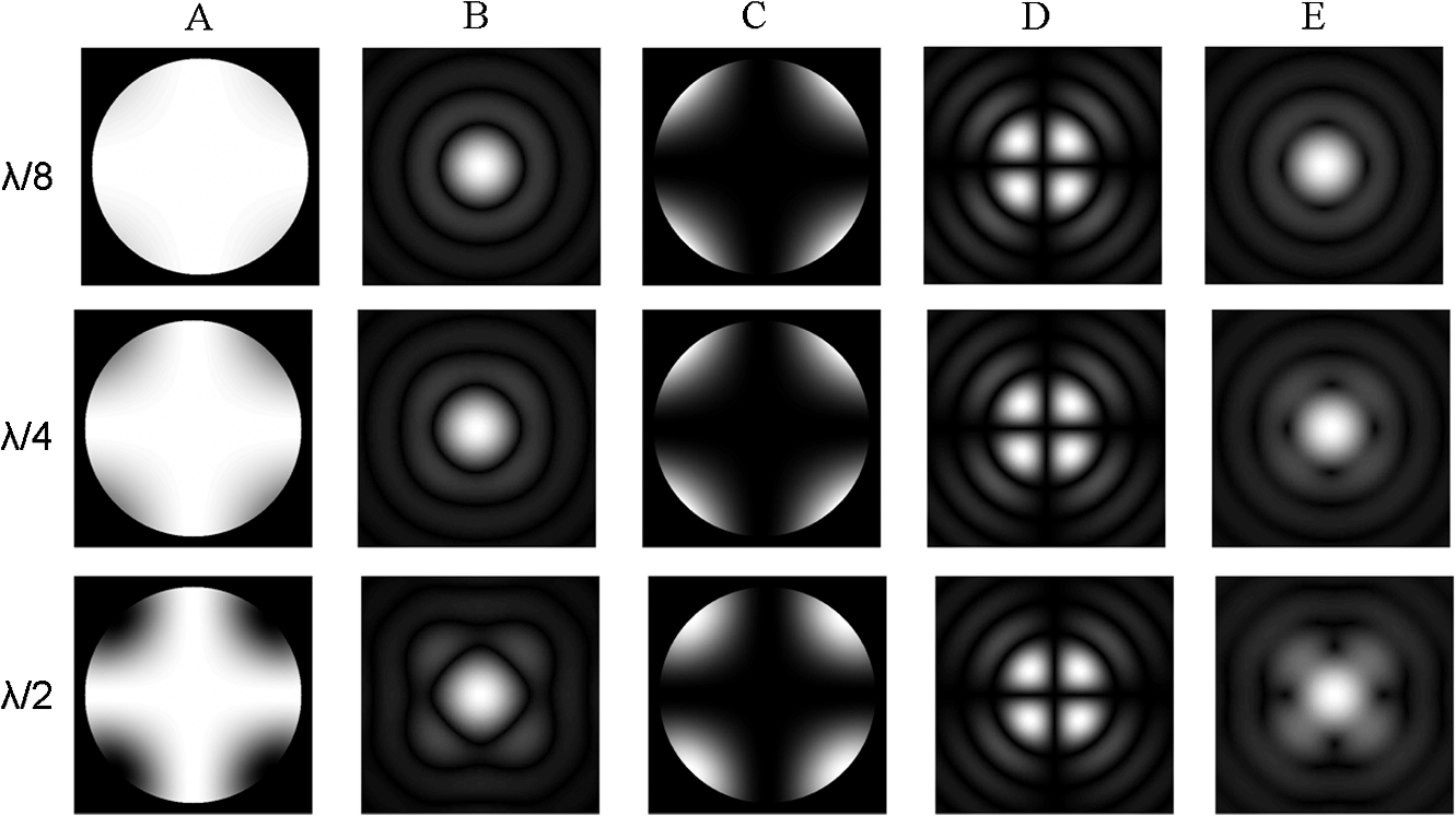

Note that the irradiance distribution for the ${\vec{E}}^{o}$ field at the exit pupil is reminiscent of the irradiance distribution under crossed polarizers of a lens that contributes diattenuation. However, in the former case, the pattern resembling a cross appears illuminated (see case A for $Δ δ = λ / 2$ ) and in the latter case the pattern appears dark.

A more realistic case is when the astigmatism term $Δ δ_{b} (\vec{H}, \vec{ρ}) = Δ δ_{1} {(\vec{a} \cdot \vec{ρ})}^{2}$ is present. Then, the irradiance patterns as calculated at the medial focus change as shown in Fig. 5. Note that for a retardance $Δ δ = λ / 4$ , there is a significant change in the point spread function as calculated at medial focus.

Fig. 5

Three cases of retardance, $Δ δ = λ / 8$ , $Δ δ = λ / 4$ , and $Δ δ = λ / 2$ . For the field ${\vec{E}}^{o}$ column A gives the irradiance at the exit pupil and column B gives the point spread function calculated at medial focus. For the field ${\vec{E}}^{e}$ column C gives the irradiance and column D gives the point spread function calculated at medial focus. Column E gives the incoherent sum of columns B and D.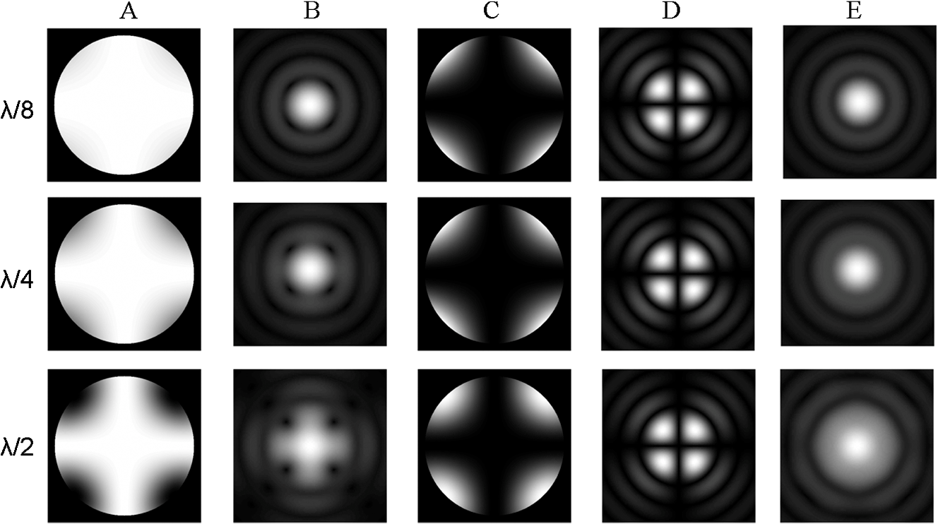

8. Elliptical Polarizaiton

In the presence of retardance, the state of polarization of a linearly polarized field changes to elliptical polarization. It is also of interest to determine the properties of the polarization ellipse.

Using the definitions,

Eq. (35)

\tan (α) = \frac{| {\vec{E}}^{e} |}{| {\vec{E}}^{o} |},

Eq. (36)

\tan (χ) = \mp \frac{b}{a} .

We write the relationships for the orientation and ellipticity of the polarization ellipse,

Eq. (37)

\tan (2 ψ) = \tan (2 α) \cos (\frac{2 π}{λ} Δ δ_{d}),

Eq. (38)

\sin (2 χ) = \sin (2 α) \sin (\frac{2 π}{λ} Δ δ_{d}),

where

ψ

is the angle that the major axis of the polarization ellipse makes with the

\vec{a}

direction, and the ellipticity

\tan (χ)

is the ratio of the minor

b

to major axis

a

of the polarization ellipse.

We can approximate the tangent of $α$ to second order by

Eq. (39)

\tan (α) = \frac{| {\vec{E}}^{e} |}{| {\vec{E}}^{o} |} ≅ \frac{2 π}{λ} Δ δ_{c} .

The retardance $Δ δ_{d}$ is given by

Eq. (40)

Δ δ_{d} = Δ δ_{b} (\vec{H}, \vec{ρ}) - \frac{1}{2} Δ δ_{a} (\vec{H} \cdot \vec{ρ}) - \frac{λ}{4} .

Then, we can write

Eq. (41)

\cos (\frac{2 π}{λ} Δ δ_{d}) = \sin {\frac{2 π}{λ} [Δ δ_{b} (\vec{H}, \vec{ρ}) - \frac{1}{2} Δ δ_{a} (\vec{H} \cdot \vec{ρ})]} ≅ \frac{2 π}{λ} [Δ δ_{b} (\vec{H}, \vec{ρ}) - \frac{1}{2} Δ δ_{a} (\vec{H} \cdot \vec{ρ})],

which is a second-order quantity. Similarly, the parameter

α

to second order is given by

Eq. (42)

α ≅ \frac{2 π}{λ} Δ δ_{c} (\vec{H}, \vec{ρ}) = \frac{2 π}{λ} [\begin{array}{l} Δ δ_{1} (\vec{a} \cdot \vec{ρ}) (\vec{b} \cdot \vec{ρ}) + Δ δ_{2} (\vec{a} \cdot \vec{ρ}) (\vec{b} \cdot \vec{H}) + \\ Δ δ_{2} (\vec{a} \cdot \vec{H}) (\vec{b} \cdot \vec{ρ}) + Δ δ_{3} (\vec{a} \cdot \vec{H}) (\vec{b} \cdot \vec{H}) \end{array}] .

Therefore, the angle $ψ$ is a fourth-order quantity implying that for a small amount of retardance $Δ δ$ the orientation of the polarization ellipse is not too different from the orientation of the field amplitude ${\vec{A}}^{'} (\vec{H}, \vec{ρ})$ .

For $\sin [(2 π / λ) Δ δ_{d}]$ , we can write to second order of approximation

Eq. (43)

\sin (\frac{2 π}{λ} Δ δ_{d}) ≅ 1 .

Then, the ellipticity for small amounts of retardance $Δ δ$ can be approximated to second order by

Eq. (44)

\tan (χ) = \frac{b}{a} ≅ \frac{2 π}{λ} [\begin{array}{l} Δ δ_{1} (\vec{a} \cdot \vec{ρ}) (\vec{b} \cdot \vec{ρ}) + Δ δ_{2} (\vec{a} \cdot \vec{ρ}) (\vec{b} \cdot \vec{H}) + \\ Δ δ_{2} (\vec{a} \cdot \vec{H}) (\vec{b} \cdot \vec{ρ}) + Δ δ_{3} (\vec{a} \cdot \vec{H}) (\vec{b} \cdot \vec{H}) \end{array}] .

For the zero field position $\vec{H} = 0$ , the ellipticity is maximum when the aperture vector $\vec{ρ}$ is at an angle of 45 deg with respect to the vector $\vec{a}$ , and at the edge of the aperture $| \vec{ρ} | = 1$ . In this case, we can write

Eq. (45)

\frac{b}{a} ≅ \frac{π}{λ} Δ δ_{1} .

For the case of having $Δ δ_{1} = λ / 10$ , the ellipticity is estimated to be 0.314. Figure 6 left shows a polarization pupil map for a refractive system with no coatings and therefore no retardance $Δ δ_{1} = 0$ . However, when the lens surfaces are coated, retardance is introduced and the polarization state changes to elliptical as shown with ellipses in Fig. 6 right.

Fig. 6

(a) Polarization pupil map showing the orientation and magnitude of the field at the exit pupil of a lens system. At the entrance pupil the field is uniform and linearly polarized. (b) When coatings are added to the surfaces retardance is introduced and the polarization state changes from linear to elliptical as shown by ellipses.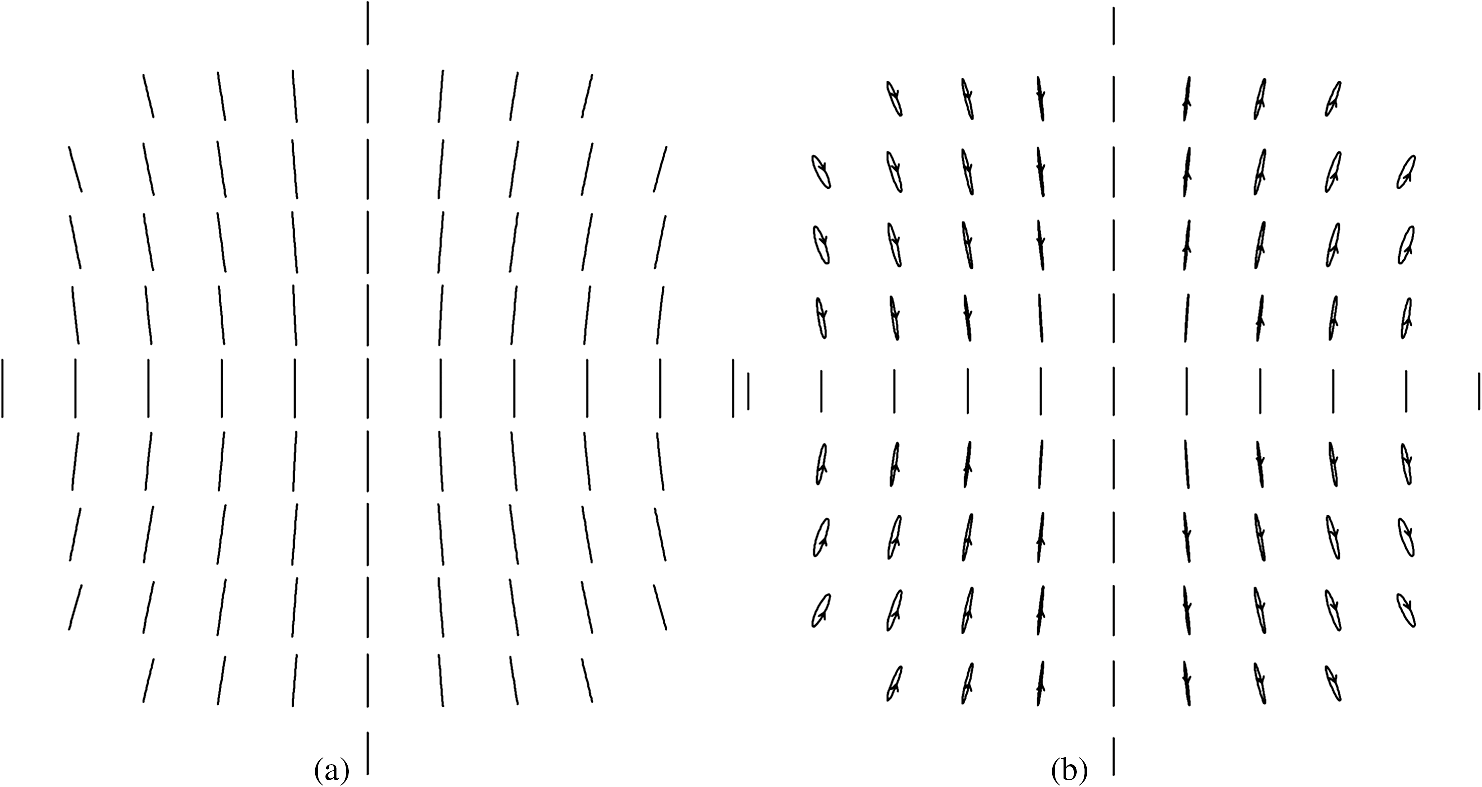

9. Summary

A useful way to understand polarization aberrations is by the concepts of polarization fields and of wavefronts of two sheets. In this article, we have constructed polarization fields requiring smoothness, symmetry properties, and physical plausibility. To this end, we have used the aberration function of a plane symmetrical system and have taken the gradient to pass from a scalar field to a vector field. We have thus defined the ${\vec{R}}_{n}$ and ${\vec{T}}_{n}$ fields as an adequate basis to describe polarization fields. These fields carry both aperture and field dependence. For completeness purposes, we have presented the first 63 ${\vec{R}}_{n}$ and ${\vec{T}}_{n}$ fields. However, given an axially symmetric system and a linear input polarization state, one would be mostly concerned with the seven third-order ${\vec{R}}_{n}$ fields ( ${\vec{R}}_{6}$ to ${\vec{R}}_{12}$ ). If the input polarization state is radial, then one would be mostly concerned with the six third-order ${\vec{R}}_{n}$ fields ( ${\vec{R}}_{13}$ to ${\vec{R}}_{18}$ ). Higher-order fields represent higher-order amplitude polarization aberrations.

For an axially symmetric system, we have expressed to second order the optical field at the exit pupil as a superposition of polarization field components. We also have provided the coefficients of these fields as a function of the system parameters and have used sums over the system surfaces to find the polarization aberration coefficients for the entire system. Data from a first-order marginal and chief ray is used to compute the polarization aberration coefficients.

In the absence of retardance $Δ δ = 0$ introduced by an optical surface, the field amplitude changes its orientation and magnitude. In addition, the first-order properties of the system change as the optical phase changes according to the function $δ (\vec{H}, \vec{ρ})$ , which represents change of focus, change of magnification, and piston aberrations.

In the presence of retardance $Δ δ \neq 0$ , the incoming optical field is split into two field components ${\vec{E}}^{o}$ and ${\vec{E}}^{e}$ . Each of these components is perpendicular to the other, and for a given optical path length, a wavefront of two sheets is defined. In addition, the phenomenon of elliptical polarization takes place. For small amounts of retardance, the orientation of the polarization ellipse is a fourth-order quantity and substantially coincides with the orientation of the transmitted field amplitude. The ellipticity is however a second-order quantity and is proportional to the amount of retardance.

The treatment presented in this article is based on previous work, and it is a refinement in that it provides analytically and graphically up to the first 63 ${\vec{R}}_{n}$ and ${\vec{T}}_{n}$ fields. Most importantly, this article highlights the occurrence of a wavefront of two sheets. In the treatment presented here. the phase calculation avoids a linear approximation to the exponential function and shows that the optical field is split into two mutually orthogonal components that would produce two distinct images. We also illustrate the amplitude apodization for the two mutually perpendicular fields and the point spread function due to both fields. Effectively, in the presence of retardance, an incoming beam is split into two beams and therefore accounting for the effects from each beam is of relevance.

The understanding of the classic aberrations of spherical, coma, astigmatism, field curvature, and distortion often presents difficulties. The case of understanding polarization aberrations can be more challenging. However, with the concepts of polarization fields and wavefront of two sheets, the understanding of polarization aberrations is eased, and simplicity and useful insights are gained. This article aims at providing a theoretical foundation to ease the understanding of polarization aberrations for optical engineering applications.

Appendices

Appendix A

Figure 7 shows a graphical display of the ${\vec{R}}_{1}$ to ${\vec{R}}_{63}$ fields.

Fig. 7

Graphical display of the ${\vec{R}}_{1}$ to ${\vec{R}}_{63}$ fields.

Appendix B

Figure 8 shows a graphical display of the ${\vec{T}}_{1}$ to ${\vec{T}}_{63}$ fields.

Fig. 8

Graphical display of the ${\vec{T}}_{1}$ to ${\vec{T}}_{63}$ fields.

Appendix C

This appendix provides some algebraic steps in obtaining the optical field. We start with the expression for the ${\vec{E}}^{*}$ field

Eq. (46)

{\vec{E}}^{*} = \exp {i \frac{2 π}{λ} [\frac{1}{2} Δ δ A^{2} (\vec{ρ} \cdot \vec{ρ})]} {\begin{cases} [{(\vec{a} \cdot \vec{t})}^{2} {\vec{E}}^{'} + (\vec{a} \cdot \vec{t}) (\vec{b} \cdot \vec{t}) {\vec{E}}^{' ⊥}] \exp [- i \frac{2 π}{λ} \frac{1}{2} Δ δ A^{2} (\vec{ρ} \cdot \vec{ρ})] + \\ [{(\vec{a} \cdot \vec{r})}^{2} {\vec{E}}^{'} + (\vec{a} \cdot \vec{r}) (\vec{b} \cdot \vec{r}) {\vec{E}}^{' ⊥}] \exp [i \frac{2 π}{λ} \frac{1}{2} Δ δ A^{2} (\vec{ρ} \cdot \vec{ρ})] \end{cases}} .

The field ${\vec{E}}^{o}$ is

Eq. (47)

{\vec{E}}^{o} = \exp {i \frac{2 π}{λ} [δ A^{2} (\vec{ρ} \cdot \vec{ρ}) + \frac{1}{2} Δ δ A^{2} (\vec{ρ} \cdot \vec{ρ})]} {\vec{E}}^{'} {\begin{cases} {(\vec{a} \cdot \vec{t})}^{2} \exp [- i \frac{2 π}{λ} \frac{1}{2} Δ δ A^{2} (\vec{ρ} \cdot \vec{ρ})] + \\ {(\vec{a} \cdot \vec{r})}^{2} \exp [i \frac{2 π}{λ} \frac{1}{2} Δ δ A^{2} (\vec{ρ} \cdot \vec{ρ})] \end{cases}} .

By expressing the exponential function with a cosine and a sine term, we can write

Eq. (48)

{\vec{E}}^{0} = \exp {i \frac{2 π}{λ} [δ A^{2} (\vec{ρ} \cdot \vec{ρ}) + \frac{1}{2} Δ δ A^{2} (\vec{ρ} \cdot \vec{ρ})]} [\begin{array}{l} [{(\vec{a} \cdot \vec{t})}^{2} {\vec{E}}^{'}] (\cos {- \frac{2 π}{λ} \frac{1}{2} [Δ δ A^{2} (\vec{ρ} \cdot \vec{ρ})]} - i \sin {\frac{2 π}{λ} \frac{1}{2} [Δ δ A^{2} (\vec{ρ} \cdot \vec{ρ})]}) + \\ [{(\vec{a} \cdot \vec{r})}^{2} {\vec{E}}^{'}] (\cos {\frac{2 π}{λ} \frac{1}{2} [Δ δ A^{2} (\vec{ρ} \cdot \vec{ρ})]} + i \sin {\frac{2 π}{λ} \frac{1}{2} [Δ δ A^{2} (\vec{ρ} \cdot \vec{ρ})]}) \end{array}] .

Or,

Eq. (49)

{\vec{E}}^{0} = \exp {i \frac{2 π}{λ} [δ A^{2} (\vec{ρ} \cdot \vec{ρ}) + \frac{1}{2} Δ δ A^{2} (\vec{ρ} \cdot \vec{ρ})]} {\vec{E}}^{'} (\cos {\frac{2 π}{λ} \frac{1}{2} [Δ δ A^{2} (\vec{ρ} \cdot \vec{ρ})]} + i \sin {\frac{2 π}{λ} \frac{1}{2} [Δ δ A^{2} (\vec{ρ} \cdot \vec{ρ})]} [{(\vec{a} \cdot \vec{r})}^{2} - {(\vec{a} \cdot \vec{t})}^{2}]) .

By expressing the complex factor in terms of its argument and phase, we can write

Eq. (50)

{\vec{E}}^{0} = {\vec{E}}^{'} \exp {i \frac{2 π}{λ} [δ A^{2} (\vec{ρ} \cdot \vec{ρ}) + \frac{1}{2} Δ δ A^{2} (\vec{ρ} \cdot \vec{ρ})]} \sqrt{(\cos^{2} {\frac{2 π}{λ} \frac{1}{2} [Δ δ A^{2} (\vec{ρ} \cdot \vec{ρ})]} + \sin^{2} {\frac{2 π}{λ} \frac{1}{2} [Δ δ A^{2} (\vec{ρ} \cdot \vec{ρ})]} {[{(\vec{a} \cdot \vec{r})}^{2} - {(\vec{a} \cdot \vec{t})}^{2}]}^{2})} \exp [i \times arct (Tan {\frac{2 π}{λ} \frac{1}{2} [Δ δ A^{2} (\vec{ρ} \cdot \vec{ρ})]} [{(\vec{a} \cdot \vec{r})}^{2} - {(\vec{a} \cdot \vec{t})}^{2}])] .

We can simplify by writing the field ${\vec{E}}^{o}$ to second order of approximation as

Eq. (51)

{\vec{E}}^{o} ≅ {\vec{E}}^{'} \exp {i \frac{2 π}{λ} [δ A^{2} (\vec{ρ} \cdot \vec{ρ}) + \frac{1}{2} Δ δ A^{2} (\vec{ρ} \cdot \vec{ρ})]} \exp (i {\frac{2 π}{λ} \frac{1}{2} [Δ δ A^{2} (\vec{ρ} \cdot \vec{ρ})]} [{(\vec{a} \cdot \vec{r})}^{2} - {(\vec{a} \cdot \vec{t})}^{2}}) = {\vec{E}}^{'} \exp {i \frac{2 π}{λ} [δ A^{2} (\vec{ρ} \cdot \vec{ρ}) + \frac{1}{2} Δ δ A^{2} (\vec{ρ} \cdot \vec{ρ})]} \exp {i [\frac{2 π}{λ} \frac{1}{2} Δ δ A^{2} (\vec{ρ} \cdot \vec{ρ})] [{(\vec{a} \cdot \vec{r})}^{2} - {(\vec{a} \cdot \vec{t})}^{2}]} = {\vec{E}}^{'} \exp {i \frac{2 π}{λ} [δ A^{2} (\vec{ρ} \cdot \vec{ρ}) + \frac{1}{2} Δ δ A^{2} (\vec{ρ} \cdot \vec{ρ})]} \exp {i (\frac{2 π}{λ} \frac{1}{2} Δ δ A^{2}) [2 {(\vec{a} \cdot \vec{ρ})}^{2} - {(\vec{a} \cdot \vec{ρ})}^{2} - {(\vec{b} \cdot \vec{ρ})}^{2}]} = {\vec{E}}^{'} \exp {i \frac{2 π}{λ} [δ A^{2} (\vec{ρ} \cdot \vec{ρ}) + Δ δ A^{2} {(\vec{a} \cdot \vec{ρ})}^{2}]} .

Let us now consider the field ${\vec{E}}^{e}$ which is

Eq. (52)

{\vec{E}}^{e} = \exp {i \frac{2 π}{λ} [δ A^{2} (\vec{ρ} \cdot \vec{ρ}) + \frac{1}{2} Δ δ A^{2} (\vec{ρ} \cdot \vec{ρ})]} {\vec{E}}^{' ⊥} {\begin{cases} (\vec{a} \cdot \vec{t}) (\vec{b} \cdot \vec{t}) \exp [- i \frac{2 π}{λ} \frac{1}{2} Δ δ A^{2} (\vec{ρ} \cdot \vec{ρ})] + \\ (\vec{a} \cdot \vec{r}) (\vec{b} \cdot \vec{r}) \exp [i \frac{2 π}{λ} \frac{1}{2} Δ δ A^{2} (\vec{ρ} \cdot \vec{ρ})] \end{cases}} .

Using the cosine and sine functions, we can write

Eq. (53)

{\vec{E}}^{e} = {\vec{E}}^{' ⊥} \exp {i \frac{2 π}{λ} [δ A^{2} (\vec{ρ} \cdot \vec{ρ}) + \frac{1}{2} Δ δ A^{2} (\vec{ρ} \cdot \vec{ρ})]} (\begin{array}{l} (\vec{a} \cdot \vec{t}) (\vec{b} \cdot \vec{t}) {\cos [\frac{2 π}{λ} \frac{1}{2} Δ δ A^{2} (\vec{ρ} \cdot \vec{ρ})] - i \sin [\frac{2 π}{λ} \frac{1}{2} Δ δ A^{2} (\vec{ρ} \cdot \vec{ρ})]} + \\ (\vec{a} \cdot \vec{r}) (\vec{b} \cdot \vec{r}) {\cos [\frac{2 π}{λ} \frac{1}{2} Δ δ A^{2} (\vec{ρ} \cdot \vec{ρ})] + i \sin [\frac{2 π}{λ} \frac{1}{2} Δ δ A^{2} (\vec{ρ} \cdot \vec{ρ})]} \end{array}) .

The cosine terms cancel and we obtain

Eq. (54)

{\vec{E}}^{e} = {\vec{E}}^{' ⊥} \exp {i \frac{2 π}{λ} [δ A^{2} (\vec{ρ} \cdot \vec{ρ}) + \frac{1}{2} Δ δ A^{2} (\vec{ρ} \cdot \vec{ρ})]} \times [2 (\vec{a} \cdot \vec{r}) (\vec{b} \cdot \vec{r})] i \sin [\frac{2 π}{λ} \frac{1}{2} Δ δ A^{2} (\vec{ρ} \cdot \vec{ρ})] = {\vec{E}}^{' ⊥} \exp {i \frac{2 π}{λ} [δ A^{2} (\vec{ρ} \cdot \vec{ρ}) + \frac{1}{2} Δ δ A^{2} (\vec{ρ} \cdot \vec{ρ}) + \frac{λ}{4}]} \times [2 (\vec{a} \cdot \vec{r}) (\vec{b} \cdot \vec{r})] \sin [\frac{2 π}{λ} \frac{1}{2} Δ δ A^{2} (\vec{ρ} \cdot \vec{ρ})] ≅ {\vec{E}}^{' ⊥} \exp {i \frac{2 π}{λ} [δ A^{2} (\vec{ρ} \cdot \vec{ρ}) + \frac{1}{2} Δ δ A^{2} (\vec{ρ} \cdot \vec{ρ}) + \frac{λ}{4}]} \times [\frac{2 π}{λ} Δ δ A^{2} (\vec{a} \cdot \vec{ρ}) (\vec{b} \cdot \vec{ρ})],

which is the expression given above.

Acknowledgments

I would like to thank Chia-Ling Li for generating the figures presented in this article. We thank Cambridge University Press for kind permission to reproduce Fig. 1, Fig. 3, and Fig. 6 and some text in Sec. 2 and Sec. 8 that were first published in Introduction to Aberrations in Optical Imaging Systems, by José Sasián, Copyright © 2013 Jose Sasian.

References

1.

M. ShribakS. InouéR. Oldenbourg, “Polarization aberrations caused by differential transmission and phase shift in high-numerical-aperture lenses: theory, measurement, and rectification,” Opt. Eng., 41 (5), 943 –954 (2002). http://dx.doi.org/10.1117/1.1467669 OPEGAR 0091-3286 Google Scholar

2.

H. KubotaS. Inoue, “Diffraction images in the polarizing microscope,” J. Opt. Soc. Am., 49 (2), 191 –198 (1959). http://dx.doi.org/10.1364/JOSA.49.000191 JOSAAH 0030-3941 Google Scholar

3.

E.W. HansenJ. A. ConchelloR. D. Allen, “Restoring image quality in the polarizing microscope: analysis of the Allen video-enhanced contrast method,” J. Opt. Soc. Am. A, 5 (11), 1836 –1847 (1988). http://dx.doi.org/10.1364/JOSAA.5.001836 JOAOD6 0740-3232 Google Scholar

4.

D. J. ReileyR. A. Chipman, “Coating-induced wave-front aberrations: on-axis astigmatism and chromatic aberration in all-reflecting systems,” Appl. Opt., 33 (10), 2002 –2012 (1994). http://dx.doi.org/10.1364/AO.33.002002 APOPAI 0003-6935 Google Scholar

5.

C. Lianget al., “Multilayer-coating-induced aberrations in extreme-ultraviolet lithography optics,” Appl. Opt., 40 (1), 129 –135 (2001). http://dx.doi.org/10.1364/AO.40.000129 APOPAI 0003-6935 Google Scholar

6.

Y. Unno, “Point-spread function for a rotationally symmetric birefringent lens,” J. Opt. Soc. Am. A, 19 (4), 981 –991 (2002). http://dx.doi.org/10.1364/JOSAA.19.000781 JOAOD6 0740-3232 Google Scholar

7.

J. RuoffM. Totzeck, “Orientation Zernike polynomials: a useful way to describe polarization effects of optical imaging systems,” J. Micro Nanolith., 8 (3), 031404 (2009). http://dx.doi.org/10.1117/1.3173803 Google Scholar

8.

N. ClarkJ. B. Breckinridge, “Polarization compensation of Fresnel aberrations in telescopes,” Proc. SPIE, 8146 814600 (2011). http://dx.doi.org/10.1117/12.896638 PSISDG 0277-786X Google Scholar

9.

R. A. ChipmanL. J. Chipman, “Polarization aberration diagrams,” Opt. Eng., 28 (2), 100 –106 (1989). http://dx.doi.org/10.1117/12.7976915 OPEGAR 0091-3286 Google Scholar

10.

J. P. McGuireR. A. Chipman, “Polarization aberrations. 1. Rotationally symmetric optical systems,” Appl. Opt., 33 (22), 5080 –5100 (1994). http://dx.doi.org/10.1364/AO.33.005080 APOPAI 0003-6935 Google Scholar

11.

J. Sasián, Introduction to Aberrations in Optical Imaging Systems, 225 –245 Cambridge University Press, Cambridge (2013). Google Scholar

12.

J. Sasián, “How to approach the design of a bilateral symmetric optical system,” Opt. Eng., 33 (6), 2045 –2061 (1994). http://dx.doi.org/10.1117/12.169736 OPEGAR 0091-3286 Google Scholar

13.

C. ZhaoJ. H. Burge, “Orthonormal vector polynomials in a unit circle, Part II: completing the basis set,” Opt. Express, 16 (9), 6586 –6591 (2008). http://dx.doi.org/10.1364/OE.16.006586 OPEXFF 1094-4087 Google Scholar

14.

J. Sasian, “Extrinsic aberrations in optical imaging systems,” Adv. Opt. Tech., 2 (1), 75 –80 (2013). http://dx.doi.org/10.1515/aot-2012-0073 2192-8576 Google Scholar

15.

R. A. Chipman, “Polarization aberrations,” The University of Arizona, (1987). Google Scholar

Biography

Jose Sasian is a professor at the College of Optical Sciences, at the University of Arizona. His research interests are in light propagation, optical design, fabrication, and testing; lens systems, opto-mechanics, light in gemstones, lithography, visual optics, optics education, and art in optics and optics in art.

CC BY: © The Authors. Published by SPIE under a Creative Commons Attribution 4.0 Unported License. Distribution or reproduction of this work in whole or in part requires full attribution of the original publication, including its DOI.

Citation Download Citation

José Sasián "Polarization fields and wavefronts of two sheets for understanding polarization aberrations in optical imaging systems," Optical Engineering 53(3), 035102 (17 March 2014). https://doi.org/10.1117/1.OE.53.3.035102

Published: 17 March 2014

Access the abstract

JOURNAL ARTICLE
15 PAGES

DOWNLOAD PAPER SAVE TO MY LIBRARY