Signal reconstruction from partial information of discrete linear canonical transform

Feng Zhang; Yang Hu; Ran Tao; Yue Wang

doi:10.1117/1.OE.53.3.034105

20 March 2014 Signal reconstruction from partial information of discrete linear canonical transform

Feng Zhang, Yang Hu, Ran Tao, Yue Wang

Author Affiliations +

Optical Engineering, Vol. 53, Issue 3, 034105 (March 2014). https://doi.org/10.1117/1.OE.53.3.034105

Abstract

Signal reconstruction, especially for nonstationary signals, occurs in many applications such as optical astronomy, electron microscopy, and x-ray crystallography. As a potent tool to analyze the nonstationary signals, the linear canonical transform (LCT) describes the effect of quadratic phase systems on a wavefield and generalizes many optical transforms. The reconstruction of a finite discrete-time signal from the partial information of its discrete LCT and some known samples under some restrictions is presented. The partial information about its discrete LCT that we have assumed to be available is the discrete LCT phase alone or the discrete LCT magnitude alone. Besides, a reconstruction example is provided to verify the effectiveness of the proposed algorithm.

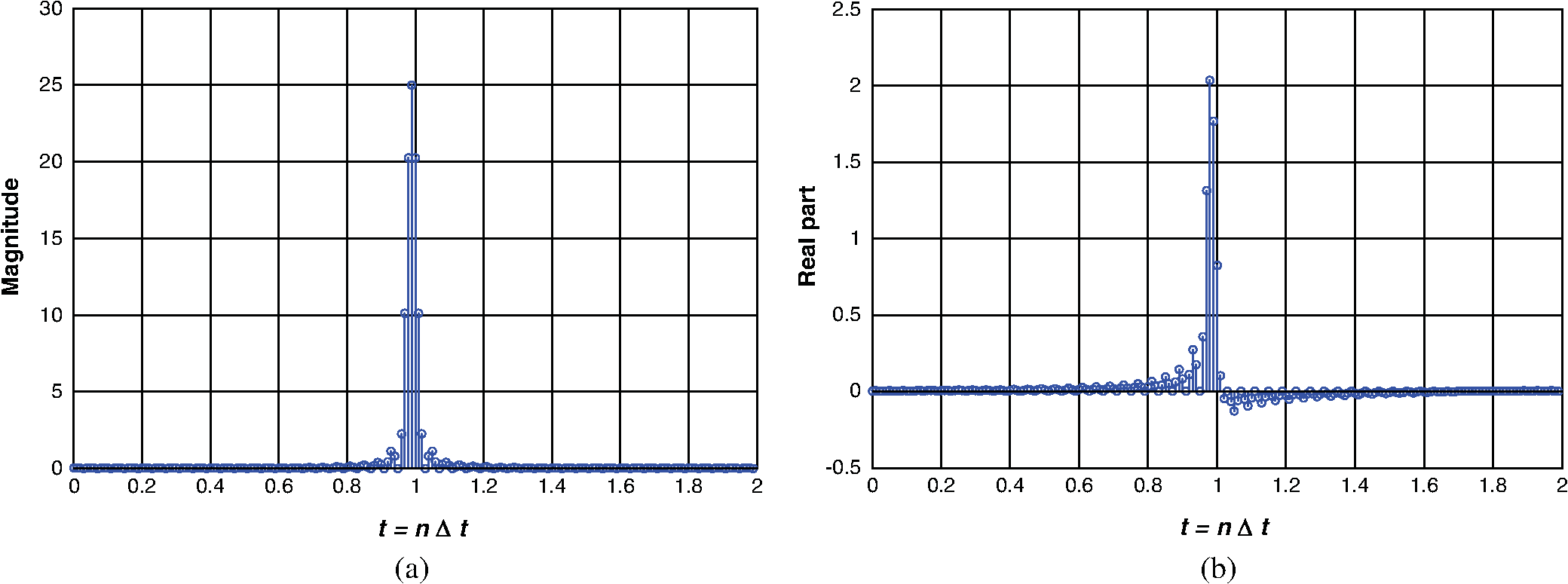
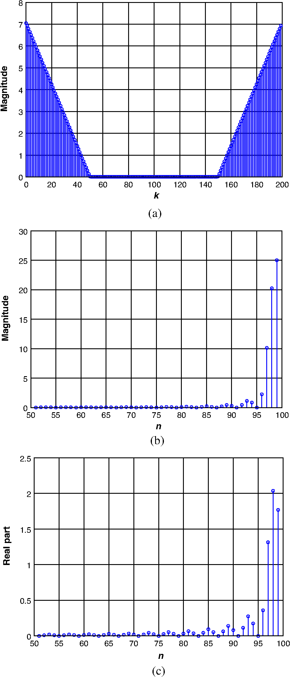
1. Introduction

Signal reconstruction, especially for nonstationary signals, plays an important role in optical signal processing and evokes considerable interest in these literatures.¹^,² In many applications, such as optical astronomy,³ electron microscopy, and x-ray crystallography,⁴ it is desired to reconstruct a complete sequence from incomplete information about the signal. The incomplete information that we have assumed to be available is usually the Fourier transform (FT) phase or the FT magnitude. Generally, a signal cannot be uniquely specified only from its FT magnitude or phase unless there is some additional information. Early works⁵^–⁷ on signal reconstruction have shown that a finite sequence can be uniquely specified by its FT magnitude with some samples under some restrictions. This reconstruction is based on an assumption that signals are band-limited in the Fourier domain. However, some nonstationary signals, such as chirp signals, are not band-limited in the Fourier domain. Applying the conventional reconstruction methods to signals nonband-limited in the Fourier domain may lead to wrong or at least suboptimal conclusions.

Since the FT is not suitable for analyzing and processing nonstationary signals, many useful tools have been introduced, such as short time FT, wavelet transform, and linear canonical transform (LCT). Among all these processing tools, the LCT, which is a linear integral transform with four parameters $(a, b, c, d)$ , has been proven to be a perfect tool in solving problems in quantum physics, optics, and nonstationary signal processing,⁸ because nonstationary signals are band-limited in the linear canonical domain. The well-known operations, such as the FT, the fractional Fourier transform (FRFT),⁸^,⁹ the Fresnel transform,¹⁰ and the scaling operation, are all special cases of the LCT. Besides, the definition and the implementation of the discrete LCT have been derived,¹¹^,¹² and have potential applications in areas of filter design, signal synthesis, phase retrieval, and pattern recognition.⁸^–¹³ Moreover, the one-dimensional (1-D) LCT is the fundamental of two-dimensional (2-D) LCT due to the separable property of 2-D LCT,¹⁴ and then we only consider the application of the 1-D LCT in first-order optical systems. Therefore, the reconstruction of nonstationary signals in the linear canonical domain is investigated in this paper.

In this paper, we present that a finite sequence can be completely reconstructed from its discrete LCT magnitude or phase and some samples under some loosen restrictions. Especially, our works are effective for nonstationary signals. The paper is organized as follows. In Sec. 2, the definitions of LCT and discrete LCT are introduced and the uniform sampling theorem for band-limited signals in the linear canonical domain is presented. In Sec. 3, the formulas to reconstruct a finite sequence from its discrete LCT magnitude or phase and some samples are derived when some conditions are known and the restrictions using in this algorithm are discussed. In addition, Sec. 4 illustrates an example. Finally, we make a conclusion in Sec. 5.

2. Preliminaries

2.1.

Linear Canonical Transform

The LCT of a continuous signal $x (t)$ with parameters $(a, b, c, d)$ is defined as⁸

Eq. (1)

X_{M} (u) = {\begin{cases} \sqrt{\frac{1}{j 2 π b}} \cdot \exp (j \frac{d}{2 b} u^{2}) \int_{- \infty}^{\infty} x (t) \exp (j \frac{a}{2 b} t^{2} - j \frac{1}{b} u t) d t, & b \neq 0 \\ \sqrt{d} e^{j \frac{c d}{2} u^{2}} x (d \cdot u), & b = 0 \end{cases},

where

M = [\begin{matrix} a & b; & c & d \end{matrix}]

is the parameter matrix and

\det (M) = a d - b c = 1

. Two successive LCTs with matrices

M_{1}

and

M_{2}

are another LCT with the matrix

M_{3} = M_{2} M_{1}

, and consequently the inverse LCT is given by the LCT with parameters (

d

,

- b

,

- c

,

a

). It is easy to verify that the LCT with parameter matrix

M = [\begin{matrix} \cos α & \sin α; & - \sin α & \cos α \end{matrix}]

reduces to the FRFT which, in specific case

α = π / 2

, becomes the FT.¹⁵^,¹⁶ The LCT also reduces to the Fresnel transform if

M = [\begin{matrix} 1 & b; & 0 & 1 \end{matrix}]

.¹⁷ The scaling operator can be viewed as a special case of the LCT with parameter matrix

M = [\begin{matrix} d^{- 1} & 0; & 0 & d \end{matrix}]

. It should be noted that when

b = 0

, the LCT of a signal is just a chirp multiplication which is of no particular interest, so we only consider the case of

b \neq 0

. Without loss of generality, we assume

b > 0

in this paper. For further details about the definitions and properties of the LCT, readers can refer to Refs. 8 9.10.11.12.13.14.15.16.–17.

2.2.

Uniform Sampling Theorem for Band-Limited Signal in the LCT Domain

A continuous signal $x (t)$ is band-limited to $Ω_{M}$ in the sense of the LCT with parameter matrix $M$ , which means that¹⁸

Eq. (2)

X_{M} (u) = 0 for | u | > Ω_{M},

where

Ω_{M}

is called the bandwidth of the signal

x (t)

in the linear canonical domain.

Lemma

Assume $x (t)$ to be band-limited to $Ω_{M}$ in the linear canonical domain with parameters $(a, b, c, d)$ , then the sampling theorem expansion for the continuous signal $x (t)$ can be expressed as¹⁹

Eq. (3)

x (t) = \exp (- j \frac{a}{2 b} t^{2}) \sum_{n = - \infty}^{+ \infty} x (n Δ t) \exp [j \frac{a}{2 b} {(n Δ t)}^{2}] sinc [\frac{Ω_{M} (t - n Δ t)}{b π}],

where

Δ t

is the sampling interval and the Nyquist rate of sampling theorem associated with the LCT is

Ω_{M} / (π b)

.

Equation (3) establishes the relationship between the signal samples and the original signals. That is to say, we can reconstruct the original signal from the uniform sampling points of the signal in the LCT domain provided that the sampling interval satisfies the uniform sampling conditions.

2.3.

Discrete Linear Canonical Transform

The uniformly sampled signal of the continuous signal $x (t)$ with sampling interval $Δ t$ is $x_{s} (t) = \sum_{n = - \infty}^{\infty} x (n Δ t) δ (t - n Δ t)$ . Here, the Dirac function $δ (t)$ is a generalized function depending on a real parameter $t$ such that it is zero for all values of the parameter except when the parameter is 0, and its integral over the parameter $t$ from $- \infty$ to $\infty$ is equal to 1. That is to say, $δ (t) = + \infty$ for $t = 0$ and $δ (t) = 0$ for $t \neq 0$ , and $\int_{- \infty}^{\infty} δ (t) d t = 1$ . Then, the LCT of the sampled signal $x_{s} (t)$ is

Eq. (4)

X_{s M} (u) = \sqrt{\frac{1}{j 2 π b}} \cdot \exp (j \frac{d}{2 b} u^{2}) \int_{- \infty}^{\infty} x_{s} (t) \exp (j \frac{a}{2 b} t^{2} - j \frac{1}{b} u t) d t = \sqrt{\frac{1}{j 2 π b}} \cdot \exp (j \frac{d}{2 b} u^{2}) \sum_{n = - \infty}^{\infty} x (n Δ t) \exp (j \frac{a}{2 b} n^{2} Δ t^{2} - j \frac{1}{b} u n Δ t) = \frac{1}{Δ t} \cdot \exp (j \frac{d}{2 b} u^{2}) \sum_{n = - \infty}^{\infty} X_{M} (u - n \frac{2 π b}{Δ t}) \exp [- j \frac{d}{2 b} {(u - n \frac{2 π b}{Δ t})}^{2}] .

Equation (4) shows that the LCT of the uniform sampled signal $x_{s} (t)$ replicates $X_{s M} (u)$ with a period of $2 π b / Δ t$ along with linear phase modulation. By sampling uniformly $N$ points in the replicated period $2 π b / Δ t$ in the linear canonical domain, the sampling interval $Δ u$ in the linear canonical domain is $Δ u = 2 π b / (N Δ t)$ . Then the discrete LCT of the discrete-time signal $x [n]$ can be defined as¹¹^,¹²

Eq. (5)

X_{M} [m] = \sqrt{1 / N} \cdot \exp (j \frac{d}{2 b} m^{2} Δ u^{2}) \sum_{n \in 〈 N 〉} x [n] \exp (j \frac{a}{2 b} n^{2} Δ t^{2} - j \frac{2 π}{N} m n) .

and the corresponding inverse transform is

Eq. (6)

x [n] = \sqrt{1 / N} \cdot \exp (- j \frac{a}{2 b} n^{2} Δ t^{2}) \sum_{m \in 〈 N 〉} X_{M} [m] \exp (- j \frac{d}{2 b} m^{2} Δ u^{2} + j \frac{2 π}{N} m n),

where

〈 N 〉

denotes the interval

[0, 1, \dots, N - 1]

without generality.

3. Reconstruction of Signals From the Partial Information Associated with the LCT

A discrete-time signal $x [n]$ can be easily reconstructed from the complete information about its discrete LCT. However, only partial information about its discrete LCT may be recorded or acquired in many practical applications. In broad terms, the partial information about its discrete LCT that we have assumed to be available is the discrete LCT phase alone or the discrete LCT magnitude alone. The attempt to reconstruct a signal exactly from its transform magnitude information is commonly referred to in the literature as the phase-retrieval problem.⁵^,²⁰ For example, the magnitude or the intensity of a diffraction pattern or an interference pattern in optical astronomy is recorded to reconstruct more complete information. Correspondingly, reconstruction from its transform phase alone is typically referred to as the magnitude-retrieval problem. Although both of these are of potential practical importance, the discrete LCT magnitude or phase alone is, in general, not sufficient to uniquely specify a discrete-time signal. So some additional information and restrictions need to be added to ensure adequate information for the reconstruction of a discrete-time signal. One way is to add some information to frequency domain, such as a bit of phase in the reconstruction of a sequence by its transform magnitude.²¹ The other way is to add some known samples in the time domain which can be obtained more easily than other ways.²² Therefore, the reconstruction of a discrete-time signal from its discrete LCT magnitude or phase and some known samples under some restrictions needs to be considered.

Suppose a continuous-time signal $x (t)$ , whose most energy is concentrated in a narrow time range $T$ , is band-limited to $Ω_{M}$ in the linear canonical domain with parameter $M = [\begin{matrix} a & b; & c & d \end{matrix}]$ . The signal is sampled uniformly by a sampling rate $f_{s} = 1 / Δ t$ in the time range $T$ , then we can obtain a sampled signal $x [n]$ where the number of samples is $N = T f_{s}$ . Without loss of generality, we suppose that the number of samples $N$ is even.

The discrete LCT of the sampled signal, $x [n]$ , for $n = 0, 1, 2, \dots, N - 1$ , is given by

Eq. (7)

X_{M} [m] = \sqrt{1 / N} \cdot \exp (j \frac{d}{2 b} m^{2} Δ u^{2}) \sum_{n = 0}^{N - 1} x [n] \exp (j \frac{a}{2 b} n^{2} Δ t^{2} - j \frac{2 π}{N} m n),

where

x [n] = x (n Δ t)

for all

n

. Since the magnitude of

X_{M} [m]

is only related to the magnitude of

\sum_{n = 0}^{N - 1} x [n] \exp (j \frac{a}{2 b} n^{2} Δ t^{2} - j \frac{2 π}{N} m n),

we can rewrite it as

\sum_{n = 0}^{N - 1} x [n] \exp (j \frac{a}{2 b} n^{2} Δ t^{2} - j \frac{2 π}{N} m n) = | \sum_{n = 0}^{N - 1} x [n] \exp (j \frac{a}{2 b} n^{2} Δ t^{2} - j \frac{2 π}{N} m n) | \exp (j θ [m]) .

Then, Eq. (7) becomes

Eq. (8)

X_{M} [m] = \sqrt{1 / N} \cdot \exp (j \frac{d}{2 b} m^{2} Δ u^{2}) | \sum_{n = 0}^{N - 1} x [n] \exp (j \frac{a}{2 b} n^{2} Δ t^{2} - j \frac{2 π}{N} m n) | \exp (j θ [m]) = \sqrt{1 / N} \cdot | \sum_{n = 0}^{N - 1} x [n] \exp (j \frac{a}{2 b} n^{2} Δ t^{2} - j \frac{2 π}{N} m n) | \exp [j (θ [m] + \frac{d}{2 b} m^{2} Δ u^{2})] = | X_{M} [m] | \exp (j θ_{M} [m]) .

Therefore, the magnitude of $X_{M} [m]$ can be defined as

Eq. (9)

| X_{M} [m] | = \sqrt{1 / N} \cdot | \sum_{n = 0}^{N - 1} x [n] \exp (j \frac{a}{2 b} n^{2} Δ t^{2} - j \frac{2 π}{N} m n) |

and the phase of

X_{M} [m]

can be expressed as

Eq. (10)

θ_{M} [m] = θ [m] + \frac{d}{2 b} m^{2} Δ u^{2} + 2 π D,

where

D

means an integer. For the special case when

m = 0

, it gives

X_{M} [0] = \sqrt{1 / N} \cdot \sum_{n = 0}^{N - 1} x [n] \exp (j \frac{a}{2 b} n^{2} Δ t^{2}) = | X_{M} [0] | .

By replacing

m

in Eq. (7) with

N - m

, the discrete LCT of

x [n]

is expressed as follows:

Eq. (11)

X_{M} [N - m] = \sqrt{1 / N} \cdot \exp [j \frac{d}{2 b} {(N - m)}^{2} Δ u^{2}] \sum_{n = 0}^{N - 1} x [n] \exp [j \frac{a}{2 b} n^{2} Δ t^{2} - j \frac{2 π}{N} (N - m) n] = \sqrt{1 / N} \cdot | \sum_{n = 0}^{N - 1} x [n] \exp [j \frac{a}{2 b} n^{2} Δ t^{2} - j \frac{2 π}{N} (N - m) n] | \exp [j (θ [N - m] + \frac{d}{2 b} {(N - m)}^{2} Δ u^{2})] = | X_{M} [N - m] | \exp (j θ_{M} [N - m]) .

The Parseval relation and energy-preserving property can be viewed as consequences of the fact that the LCT is based on a set of orthonormal basis functions.¹⁴^,²³ Due to the energy-preserving property of the LCT, the squared LCT magnitude is often called the linear canonical energy spectrum of the signal and can be interpreted as the distribution of the signal’s energy among the different chirps. From its discrete form, we can obtain the energy either from the finite sequence $x [n]$ or from the discrete LCT magnitude $| X_{M} [m] |$ . If we want to acquire the energy from the less samples of the discrete LCT magnitude, we can consider the even symmetry property of the discrete LCT magnitude, that is to say $| X_{M} [m] | = | X_{M} [N - m] |$ . By this way, the number of the discrete LCT magnitude in the computation of the energy can be reduced to $N / 2$ . From Eq. (9), we can deduce that this sequence $x [n] \exp [j (a / 2 b) n^{2} Δ t^{2}]$ should be real. So the choice of parameter matrix $M = [\begin{matrix} a & b; & c & d \end{matrix}]$ is associated with the continuous-time signal $x (t)$ . Note that the phase of

\sum_{n = 0}^{N - 1} x [n] \exp (j \frac{a}{2 b} n^{2} Δ t^{2} - j \frac{2 π}{N} m n)

has the odd symmetry property when the sequence

x [n] \exp [j (a / 2 b) n^{2} Δ t^{2}]

is real. Using this odd property, the phase of

X_{M} [N - m]

becomes

θ_{M} [N - m] = - θ [m] + \frac{d}{2 b} {(N - m)}^{2} Δ u^{2} + 2 π D^{'},

where

D^{'}

means an integer. Because of these properties, the sequence

x [n]

can be rewritten as

Eq. (12)

x [n] = \sqrt{1 / N} \cdot \exp (- j \frac{a}{2 b} n^{2} Δ t^{2}) \sum_{m = 0}^{N - 1} X_{M} [m] \exp (- j \frac{d}{2 b} m^{2} Δ u^{2} + j \frac{2 π}{N} m n) = \sqrt{1 / N} \cdot \exp (- j \frac{a}{2 b} n^{2} Δ t^{2}) {X_{M} [0] + {(- 1)}^{n} X_{M} [\frac{N}{2}] \exp [- j \frac{d}{2 b} \cdot {(\frac{N}{2})}^{2} Δ u^{2}] + \sum_{m = 1}^{\frac{N}{2} - 1} | X_{M} [m] | (\exp [j (θ_{M} [m] - \frac{d}{2 b} m^{2} Δ u^{2}) + j \frac{2 π}{N} m n] + \exp [j (θ_{M} [N - m] - \frac{d}{2 b} {(N - m)}^{2} Δ u^{2}) - j \frac{2 π}{N} m n])} = \sqrt{1 / N} \cdot \exp (- j \frac{a}{2 b} n^{2} Δ t^{2}) {2 \sum_{m = 1}^{\frac{N}{2} - 1} | X_{M} [m] | \cos (θ [m] + \frac{2 π}{N} m n) + X_{M} [0] + {(- 1)}^{n} | X_{M} [\frac{N}{2}] | \exp (j θ [\frac{N}{2}])} .

Based on the sampling theorem for band-limited signal in the linear canonical domain, the sampling rate should be greater or equal to the Nyquist rate. That is to say, the sampling rate $f_{s}$ should be satisfied $f_{s} \geq Ω_{M} / (π b)$ . When the sampling rate $f_{s}$ satisfies $f_{s} = Ω_{M} / (π b)$ , the number of samples becomes $N = T f_{s} = T Ω_{M} / (π b)$ . Due to the fact that $x (t)$ is band-limited to $Ω_{M}$ in the linear canonical domain, the discrete LCT $X_{M} [m]$ is nonzero only in the limited band $Ω_{M}$ with the replicated period $2 π b / Δ t$ in the linear canonical domain. For the case that $m = N / 2$ , we can obtain $X_{M} [N / 2] = 0$ . Then Eq. (12) can be rewritten as

Eq. (13)

x [n] = \sqrt{1 / (T f_{s})} \cdot \exp (- j \frac{a}{2 b} n^{2} Δ t^{2}) {2 \sum_{m = 1}^{⌈ T Ω_{M} / (2 π b) - 1 ⌉} | X_{M} [m] | \cos (θ [m] + \frac{2 π}{N} m n) + | X_{M} [0] |},

where the symbol

⌈ α ⌉

represents the smallest integer greater than or equal to

α

.

When the sampling rate $f_{s}$ satisfies $f_{s} > Ω_{M} / (π b)$ , the number of samples becomes $N = T f_{s}$ and $T f_{s} > T Ω_{M} / (π b)$ . According to the relationship between the continuous form and the discrete form of the LCT, we can deduce that there are $N + 1 - ⌈ T Ω_{M} / π b ⌉$ values of the discrete LCT magnitude equal to zeros which distribute at $m = ⌈ T Ω_{M} / (2 π b) ⌉$ , $⌈ T Ω_{M} / (2 π b) ⌉ + 1, \dots, N - ⌈ T Ω_{M} / (2 π b) ⌉$ . Since this products, Eq. (12) can be rewritten as

Eq. (14)

x [n] = \sqrt{1 / (T f_{s})} \cdot \exp (- j \frac{a}{2 b} n^{2} Δ t^{2}) {2 \sum_{m = 1}^{⌈ T Ω_{M} / (2 π b) - 1 ⌉} | X_{M} [m] | \cos (θ [m] + \frac{2 π}{N} m n) + | X_{M} [0] |} .

From Eq. (14) we can obtain that the whole sequence $x [n]$ can be uniquely reconstructed by the discrete LCT magnitude $| X_{M} [m] |$ and $M$ samples of $x [n]$ if $M$ samples of $θ [m]$ can be solved uniquely, where $M$ is $⌈ T Ω_{M} / (2 π b) - 1 ⌉$ .

Rewritten Eq. (14) in matrix form

Eq. (15)

x [n] = \sqrt{1 / (T f_{s})} \cdot \exp (- j \frac{a}{2 b} n^{2} Δ t^{2}) {\sum_{m = 0}^{⌈ T Ω_{M} / (2 π b) - 1 ⌉} 2 | X_{M} [m] | A [m, n]},

where

A [m, n] = 1 / 2

for

m = 0

otherwise

A [m, n] = \cos [θ [m] + (2 π / N) m n]

. Therefore, if

Rank (A) = M

, the whole sequence

x [n]

can be uniquely reconstructed by the discrete LCT phase

θ_{M} [m]

and

M

samples of

x [n]

, where

M

is

⌈ T Ω_{M} / (2 π b) ⌉

.

It should be pointed that the obtained reconstruction process can also be completed when the initial sample is not confined to the first sample of $x [n]$ and even if the known samples are not successive. In fact, the needed known samples for completing the reconstruction is related with the total samples, which is determined by the sampling rate $f_{s}$ . When the sampling rate satisfies $f_{s} = Ω_{M} / (π b)$ , the ratio $M / N$ is approximately equal to 0.5. In other words, the number of known samples is approximately equal to $N / 2$ . Therefore, these loosen restrictions extend the scope of application of the reconstruction method greatly.

4. Simulation Results and Discussion

In many practical cases, it is much easier to obtain the discrete LCT magnitude of a sequence than its discrete LCT phase. In addition, the sampling rate is often higher than the Nyquist rate. Therefore, it is necessary to verify the validity of the reconstruction algorithm by using the discrete LCT magnitude and some samples of a sequence. In this section, an example of the reconstruction algorithm described in our work is demonstrated.

The original continuous-time signal is a squared sinc function multiplied by a phase factor $\exp [- j (a / 2 b) t^{2}]$ ,

x (t) = \frac{Ω_{0}}{2 π} {sinc [\frac{Ω_{0}}{2 π} (t - T / 2)]}^{2} \exp (- j \frac{a}{2 b} t^{2}),

where

T = 2

and

Ω_{0} = 25 π

. For a function

\frac{Ω_{0}}{2 π} {sinc (\frac{Ω_{0}}{2 π} t)}^{2} \exp (- j \frac{a}{2 b} t^{2}),

its LCT with parameter

M = [\begin{matrix} a & b; & c & d \end{matrix}]

is a triangular function. Then according to the properties of the LCT, the LCT of

x (t)

is also a triangular function and its bandwidth in the linear canonical domain is

2 Ω_{0} / b

. So the Nyquist rate of sampling theorem associated with the LCT is

Ω_{M} = 2 Ω_{0} / (π b)

.

The discrete-time signal $x [n]$ is sampled from the continuous-time signal $x (t)$ with sampling interval $Δ t = 0.01$ , that is $x [n] = x (n Δ t)$ . Here, we select the parameter $M = [\begin{matrix} 3 & 1; & 0.5 & 0.5 \end{matrix}]$ . Note that the sampling rate $f_{s} = 1 / Δ t$ is higher than the Nyquist rate $2 Ω_{0} / (π b)$ . Since the most energy of the original signal is concentrated in the narrow time range $T$ , the discrete-time signal $x [n]$ is approximated as a finite sequence in the interval [0, 2], and thus can be numerically simulated in a computer. Besides, the number of samples is $N = 200$ in the time domain.

The magnitude and real part of discrete-time signal $x [n]$ which need to be reconstructed are shown in Figs. 1(a) and 1(b), respectively. We suppose that the discrete LCT magnitude of $x [n]$ and $M$ samples of $x [n]$ are known, which are used to the reconstruction of the uniformly sampled sequence. Here, the value of $M$ is $⌈ T Ω_{M} / (2 π b) - 1 ⌉ = 49$ . This known partial information is plotted in Fig. 2. Based on Eq. (14), we can reconstruct the whole sequence $x [n]$ by the discrete LCT magnitude of $x [n]$ and 49 samples of $x [n]$ . The discrete-time signal reconstructed by the proposed algorithm is shown in Fig. 3, where the magnitude and real part of the reconstructed discrete-time signal are plotted in Figs. 3(a) and 3(b), respectively. In order to compare the reconstructed discrete-time signal with the original discrete-time signal shown in Fig. 1 more explicitly, the reconstructed sequence and the original sequence are plotted in the same figure and can be distinguished by two commonly used types of symbols in Fig. 3. It is clear from Fig. 3 that the discrete-time signal reconstructed by the proposed algorithm is exactly equal to the original discrete-time signal shown in Fig. 1. Note that the number of known samples is less than $N / 2$ and the initial known sample is not confined to be the first sample of $x [n]$ . Therefore, the reconstruction of signals from the partial information associated with the LCT works fairly well in the case of the nonstationary input under some loosen restrictions.

Fig. 1

(a) The magnitude and (b) real part of the discrete-time signal.

Fig. 2

(a) The discrete LCT magnitude of $x [n]$ with parameter $M = [\begin{matrix} 3 & 1; & 0.5 & 0.5 \end{matrix}]$ . (b) The magnitude and (c) real part of some known samples.

Fig. 3

(a) The magnitude and (b) real part of the reconstructed discrete-time signal.

5. Conclusion

In this paper, the reconstruction of a finite discrete-time signal from its discrete LCT magnitude or phase and some known samples under some restrictions has been proposed. It has been shown that the number of known samples is related to the sampling frequency and can be less than half of the total number of the finite discrete-time signal when the sampling rate is larger than the Nyquist rate. Besides, simulation results have shown the better performance of the reconstruction algorithm for nonstationary signals even when the initial known sample is not the first sample of the discrete-time signal. The proposed algorithm will promote the applications of the reconstruction of nonstationary discrete-time signals in the linear canonical domain.

Acknowledgments

This work was supported in part by the National Natural Science Foundation of China under Grant Nos. 61201354 and 61331021, by the Beijing Higher Education Young Elite Teacher Project, and by the Basic Science Foundation of Beijing Institute of Technology under Grant No. 20120542005.

References

1.

Y. Zhao et al., “Three-dimensional reconstruction of in vivo blood vessels in human skin using phase-resolved optical Doppler tomography,” IEEE J. Sel. Top. Quantum Electron., 7 (6), 931 –935 (2001). http://dx.doi.org/10.1109/2944.983296 IJSQEN 1077-260X Google Scholar

2.

K. Nitta et al., “Image reconstruction for thin observation module by bound optics by using the iterative backprojection method,” Appl. Opt., 45 (13), 2893 –2900 (2006). http://dx.doi.org/10.1364/AO.45.002893 APOPAI 0003-6935 Google Scholar

3.

J. R. Fienup, “Space object imaging through the turbulent atmosphere,” Opt. Eng., 18 (5), 185529 (1979). http://dx.doi.org/10.1117/12.7972425 OPEGAR 0091-3286 Google Scholar

4.

R. J. Read, “Improved Fourier coefficients for maps using phases from partial structures with errors,” Acta Crystallogr., Sect. A: Found. Crystallogr., 42 (3), 140 –149 (1986). http://dx.doi.org/10.1107/S0108767386099622 ACACEQ 0108-7673 Google Scholar

5.

A. V. Oppenheim, J. S. Lim and S. R. Curtis, “Signal synthesis and reconstruction from partial Fourier-domain information,” J. Opt. Soc. Am., 73 (11), 1413 –1420 (1983). http://dx.doi.org/10.1364/JOSA.73.001413 JOSAAH 0030-3941 Google Scholar

6.

M. Hayes, “The reconstruction of a multidimensional sequence from the phase or magnitude of its Fourier transform,” IEEE Trans. Acoust. Speech Signal Process., 30 (2), 140 –154 (1982). http://dx.doi.org/10.1109/TASSP.1982.1163863 IETABA 0096-3518 Google Scholar

7.

S. Nawab, T. Quatieri and J. Lim, “Signal reconstruction from short-time Fourier transform magnitude,” IEEE Trans. Acoust. Speech Signal Process., 31 (4), 986 –998 (1983). http://dx.doi.org/10.1109/TASSP.1983.1164162 IETABA 0096-3518 Google Scholar

8.

H. M. Ozaktas, Z. Zalevsky and M. A. Kutay, The Fractional Fourier Transform with Applications in Optics and Signal Processing, Wiley, New York (2001). Google Scholar

9.

F. Zhang, R. Tao and Y. Wang, “Discrete fractional Fourier transform computation by adaptive method,” Opt. Eng., 52 (6), 068202 (2013). http://dx.doi.org/10.1117/1.OE.52.6.068202 OPEGAR 0091-3286 Google Scholar

10.

D. F. James and G. S. Agarwal, “The generalized Fresnel transform and its application to optics,” Opt. Commun., 126 (4), 207 –212 (1996). http://dx.doi.org/10.1016/0030-4018(95)00708-3 OPCOB8 0030-4018 Google Scholar

11.

S. C. Pei and J. J. Ding, “Closed-form discrete fractional and affine Fourier transforms,” IEEE Trans. Signal Process., 48 (5), 1338 –1353 (2000). http://dx.doi.org/10.1109/78.839981 ITPRED 1053-587X Google Scholar

12.

F. S. Oktem and H. M. Ozaktas, “Exact relation between continuous and discrete linear canonical transforms,” IEEE Signal Process. Lett., 16 (8), 727 –730 (2009). http://dx.doi.org/10.1109/LSP.2009.2023940 IESPEJ 1070-9908 Google Scholar

13.

S. C. Pei and J. J. Ding, “Eigenfunctions of linear canonical transform,” IEEE Trans. Signal Process., 50 (1), 11 –26 (2002). http://dx.doi.org/10.1109/78.972478 ITPRED 1053-587X Google Scholar

14.

T. Alieva and M. J. Bastiaans, “Alternative representation of the linear canonical integral transform,” Opt. Lett., 30 (24), 3302 –3304 (2005). http://dx.doi.org/10.1364/OL.30.003302 OPLEDP 0146-9592 Google Scholar

15.

L. B. Almeida, “The fractional Fourier transform and time-frequency representations,” IEEE Trans. Signal Process., 42 (11), 3084 –3091 (1994). http://dx.doi.org/10.1109/78.330368 ITPRED 1053-587X Google Scholar

16.

C. Candan and H. M. Ozaktas, “Sampling and series expansion theorems for fractional Fourier and other transforms,” Signal Process., 83 (11), 2455 –2457 (2003). http://dx.doi.org/10.1016/S0165-1684(03)00196-8 SPRODR 0165-1684 Google Scholar

17.

A. Papoulis, “Pulse compression, fiber communications, and diffraction: a unified approach,” J. Opt. Soc. Am. A, 11 (1), 3 –13 (1994). http://dx.doi.org/10.1364/JOSAA.11.000003 JOAOD6 0740-3232 Google Scholar

18.

A. Stern, “Sampling of linear canonical transformed signals,” Signal Process., 86 (7), 1421 –1425 (2006). http://dx.doi.org/10.1016/j.sigpro.2005.07.031 SPRODR 0165-1684 Google Scholar

19.

B. Z. Li, R. Tao and Y. Wang, “New sampling formulae related to linear canonical transform,” Signal Process., 87 (5), 983 –990 (2007). http://dx.doi.org/10.1016/j.sigpro.2006.09.008 SPRODR 0165-1684 Google Scholar

20.

L. Taylor, “The phase retrieval problem,” IEEE Trans. Antennas Propag., 29 (2), 386 –391 (1981). http://dx.doi.org/10.1109/TAP.1981.1142559 IETPAK 0018-926X Google Scholar

21.

P. Van Hove, M. Hayes and J. Lim, “Signal reconstruction from signed Fourier transform magnitude,” IEEE Trans. Acoust. Speech Signal Process., 31 (5), 1286 –1293 (1983). http://dx.doi.org/10.1109/TASSP.1983.1164178 IETABA 0096-3518 Google Scholar

22.

S. H. Nawab, T. F. Quatieri and J. S. Lim, “Signal reconstruction from short-time Fourier transform magnitude,” IEEE Trans. Acoust. Speech Signal Process., 31 (4), 986 –998 (1983). http://dx.doi.org/10.1109/TASSP.1983.1164162 IETABA 0096-3518 Google Scholar

23.

Q. Xiang and K. Y. Qin, “The linear canonical transform and its application to time-frequency signal analysis,” in Proc. IEEE. Int. Conf. Information Engineering and Computer Science 2009, 1 –4 (2009). Google Scholar

Biography

Feng Zhang received the BS and MS degrees in communication and information systems from Zhengzhou University, Zhengzhou, China, in 2003 and 2006, and a PhD degree in information and communication engineering from Beijing Institute of Technology, Beijing, China, in 2010, respectively. Currently, he is a lecturer with the Department of Electronic Engineering, Beijing Institute of Technology. His research interests include time-frequency analysis and radar signal processing.

Yang Hu received the BS degree in communication and information systems from Zhengzhou University, Zhengzhou, China, in 2012. He is currently working toward the MS degree in information and communication engineering at the Beijing Institute of Technology. His current research interests include time-frequency analysis, ABCD transforms and discrete optical signal processing.

Ran Tao received a PhD degree in electrical engineering from Harbin Institute of Technology, Harbin, in 1993. He has been a professor at Beijing Institute of Technology since 1999. His research interests include fractional Fourier transform with applications in radar and communication systems. He is the vice president of the Chinese Radar Industry Association, and a fellow of the Chinese Institute of Electronics.

Yue Wang received the BS degree in radar engineering from Xidian University, Shaanxi, China, in 1956. He was the president of the Beijing Institute of Technology (BIT), China, from 1993 to 1997. Currently, he is a professor with BIT. His research interests include information system theory and technology, and signal processing. He is a fellow of the Chinese Academy of Sciences and also a fellow of the Chinese Academy of Engineering.

CC BY: © The Authors. Published by SPIE under a Creative Commons Attribution 4.0 Unported License. Distribution or reproduction of this work in whole or in part requires full attribution of the original publication, including its DOI.

Citation Download Citation

Feng Zhang, Yang Hu, Ran Tao, and Yue Wang "Signal reconstruction from partial information of discrete linear canonical transform," Optical Engineering 53(3), 034105 (20 March 2014). https://doi.org/10.1117/1.OE.53.3.034105

Published: 20 March 2014

Access the abstract

JOURNAL ARTICLE
8 PAGES

DOWNLOAD PAPER SAVE TO MY LIBRARY

GET CITATION

CITATIONS

Cited by 7 scholarly publications.

Explore citations on Lens.org

KEYWORDS

Reconstruction algorithms

Fourier transforms

X-ray astronomy

Optical engineering

Astronomical imaging

Astronomy

Computer simulations

1.

Introduction

2.

Preliminaries

2.1.

Linear Canonical Transform

Eq. (1)

2.2.

Uniform Sampling Theorem for Band-Limited Signal in the LCT Domain

Eq. (2)

Lemma

Eq. (3)

2.3.

Discrete Linear Canonical Transform

Eq. (4)

Eq. (5)

Eq. (6)

3.

Reconstruction of Signals From the Partial Information Associated with the LCT

Eq. (7)

Eq. (8)

Eq. (9)

Eq. (10)

Eq. (11)

Eq. (12)

Eq. (13)

Eq. (14)

Eq. (15)

4.

Simulation Results and Discussion

Fig. 1

Fig. 2

Fig. 3

5.

Conclusion

Acknowledgments

References

Biography

Show All Keywords

Keywords/Phrases

Search In:

Publication Years