Curvelet-based method for orientation estimation of particles from optical images

Jouni A. Sampo; Jouni J. Takalo; Samuli Siltanen; Arttu Miettinen; Matti Lassas; Jussi Timonen

doi:10.1117/1.OE.53.3.033109

27 March 2014 Curvelet-based method for orientation estimation of particles from optical images

Jouni A. Sampo, Jouni J. Takalo, Samuli Siltanen, Arttu Miettinen, Matti Lassas, Jussi Timonen

Author Affiliations +

Optical Engineering, Vol. 53, Issue 3, 033109 (March 2014). https://doi.org/10.1117/1.OE.53.3.033109

Abstract

A method based on the curvelet transform is introduced to estimate the orientation distribution from two-dimensional images of small anisotropic particles. Orientation of fibers in paper is considered as a particular application of the method. Theoretical aspects of the suitability of this method are discussed and its efficiency is demonstrated with simulated and real images of fibrous systems. Comparison is made with two traditionally used methods of orientation analysis, and the new curvelet-based method is shown to perform better than these traditional methods.

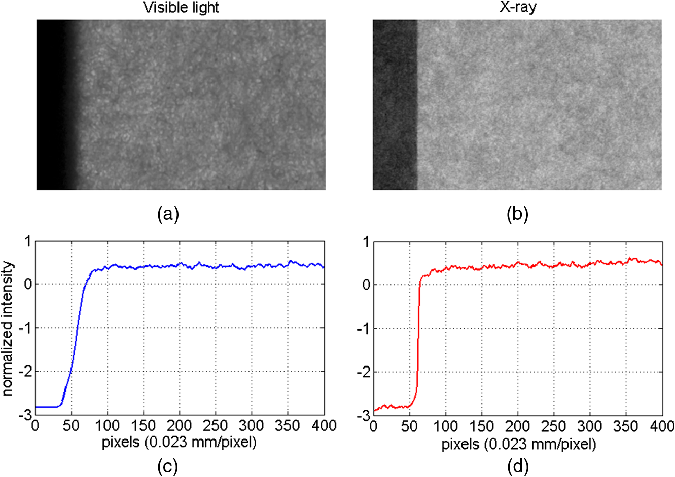
1. Introduction

Orientation analysis of complex patterns is usually done by applying the fast Fourier transform (FFT)¹ or gradient-based methods like the structure tensors (ST).²^–⁵ Relative strengths of different orientations are measured, e.g., by investigating the magnitudes of Fourier-transform coefficients usually in polar coordinates. However, during the last two decades, more sophisticated transforms, especially the wavelet transform,⁶ have become popular in many fields, where Fourier transforms have traditionally been applied. Moreover, during the last decade, transforms like the curvelet, contourlet, and shearlet transforms have been developed and have proven to be well suited for various applications.⁷^–¹⁰ The basis functions of these new transforms are tightly localized in the both space and frequency domains and have in addition a direction angle, i.e., an orientation parameter that makes them promising tools for orientation analysis.

We use in this work the orientation of fibers in paper as the basic application and framework. This choice was made because data to be analyzed in this application are common and challenging. Therefore, if the methods developed work well in this case they will probably work in many other (similar) applications such as, e.g., determination of the orientation of fibers or nanofibrils in reinforced composites.⁵^,¹¹ Furthermore, in paper-making industry it would be advantageous to have a good orientation analysis method for on-line measurements during the manufacturing process (paper webs move up to $2000 m / \min$ ).

This article is organized as follows. In Sec. 2, we discuss data typically related to the present application. In Sec. 3, the curvelet transform together with a few relevant theorems are first introduced and then the curvelet method for orientation distribution is described in Sec. 4. In Sec. 5, we apply this method to a numerically generated network of fibers with a known orientation distribution and to a newsprint and organic-fiber sample, and compare our results with those achieved by other, previously used methods for orientation analysis.

2. Optical Imaging of Fibers

In the paper-making process wood fibers, mineral fillers, and other additives together form the basic structure of paper. The properties of paper depend essentially on how fibers are distributed. For example, the so-called streakiness in its fiber orientation causes gloss variation in the high-quality printing papers.¹²^,¹³ Furthermore, different (average) orientations in different layers of paper affect its bending properties, and different orientations at its top and bottom surface make it curved.¹⁴ Even if the orientation would be similar, two sidedness in the anisotropy (the maximum to minimum ratio of the distribution) of the orientation may result into curliness of the paper sheet.¹⁵^,¹⁶ For these reasons, it would be important in the paper-making process to be able to measure, and to thereby facilitate at least the control of fiber orientation at the surface of the paper web.

Fibers in paper form a more or less random network with predominantly planar orientation of fibers. As an off-line measurement, it is possible to study also the three-dimensional fiber structure of paper with tomographic imaging,¹⁷ but this is slow and the sample needs to be very small. With CCD cameras large areas of paper (also the paper web in a running paper machine) can be imaged fast, but these images mostly reveal the planar orientation of fibers only. Fortunately, this planar information is often enough in practice and in an optimal case, determination of the planar fiber orientation would enable on-line adjustment of the paper-making process. As the camera technology keeps on developing rapidly, orientation analysis of the whole paper web is expected to become feasible fairly soon, i.e., prices of suitable cameras will be at an acceptable level for the fairly large numbers of cameras needed for an accurate enough imaging.

To make fibers more clearly visible in paper, bright-field images are preferred over reflection images. In Fig. 1, we show a bright-field image of paper, from which the orientation distribution should be determined. Notice that here fibers are clearly visible.

Fig. 1

A bright-field image of a paper sample. Sample size was about $3.4 \times 2.4 {mm}^{2}$ .

The light passing through paper is, however, strongly scattered by the abundant fiber–air interfaces (wet paper is more transparent due to a better match of the dielectric properties of water and fibers) and therefore in practice only the fibers that are close to the surface on the camera side (basically a couple layers of fibers) appear in the image (beyond that light rays “lose their memory”). We can demonstrate the “diffusive” passage of light across paper by partly eclipsing the light source with a metal tape. In an optical bright-field image of the paper, the edge of the tape appears much more blurred than in its similar image taken by x-rays (see Fig. 2). It is evident that from bright-field images only the (near-) surface orientation of fibers can be determined, which must be taken into account in practical applications. For example, orientation of fibers at and near the surface does not alone explain the strength of the paper, but is important, e.g., for its printing properties.

Fig. 2

Blurring of a sharp edge in the transmission of visible light (a) and x-rays (b) through paper. Normalized intensity of the transmission intensity of visible light (c) and x-rays (d).

3. Mathematical Methods

3.1.

Curvelet Transform

There exist different constructions of a continuous curvelet transform (CCT). We review here the one presented by Candès and Donoho,¹⁸^,¹⁹ since it displays most clearly the essential properties of this transform.

The CCT is defined in polar coordinates $(r, ω)$ of the frequency domain. Let $W$ be a non-negative, infinitely smooth real-valued function supported inside the interval ( $1 / 2$ , 2), called the “radial window.” Furthermore, let $V$ be a non-negative, infinitely smooth real-valued function supported in the interval $[- 1, 1]$ called the “angular window.” We assume the following admissibility conditions:

Eq. (1)

\int_{0}^{\infty} W {(r)}^{2} \frac{d r}{r} = 1 and \int_{- 1}^{1} V {(ω)}^{2} d ω = 1 .

We use in the following a positive parameter, $a$ , called the “scale.” At each scale $0 < a < a_{0}$ , the so-called “mother curvelet,” $γ_{a 00}$ is defined in the frequency domain by

Eq. (2)

{\hat{γ}}_{a 00} [r \cos (ω), r \sin (ω)] = a^{\frac{3}{4}} W (a r) V (ω / \sqrt{a}),

where

r \geq 0

and

ω \in [0, 2 π)

. Now,

{\hat{γ}}_{a 00}

is supported in the frequency domain as illustrated in Fig. 3. The spatial-domain mother curvelet,

γ_{a 00}

is determined from Eq. (2) by an inverse Fourier transform.

Fig. 3

Support of ${\hat{γ}}_{a b θ}$ in the frequency domain (a), and the area that contains most of the “energy” of $γ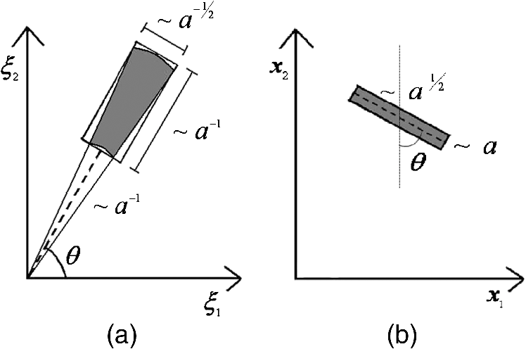_{a b θ}$ (b).

Now, a rotation parameter, $θ \in [0, 2 π)$ , and a translation parameter, $b \in R^{2}$ , are included so as to end up with a definition for the whole “curvelet,” $γ_{a b θ}$ :

Eq. (3)

γ_{a b θ} (x) = γ_{a 00} [R_{- θ} (x - b)], for x \in R^{2},

where

R_{θ}

is the matrix of a planar counter-clockwise rotation by angle

θ

. The curvelet transform,

Γ_{f} (a, b, θ)

of

f

, is then defined by

Eq. (4)

Γ_{f} (a, b, θ) := 〈 γ_{a b θ}, f 〉 = \int_{R^{2}} f (x) γ_{a b θ} (x) d x

for all

0 < a < a_{0}

,

b \in R^{2}

, and

θ \in [0, 2 π)

.

Notice that the curvelet transform has also an inverse transform, although we do not need it in our application.

Because of the compact support of ${\hat{γ}}_{a b θ}$ , the support of $γ_{a b θ}$ cannot be compact. However, $γ_{0 b θ} (x)$ and its derivatives decay rapidly when $x$ moves away from $b$ ,²⁰ i.e., $γ_{a b θ}$ is well localized around $b$ . Therefore, one would then expect that it would adapt well to short and thin objects like fibers.

As illustrated in Fig. 3 that rotation parameter $θ$ is the angle between the $x_{2}$ axis and the major axis (orientation) of $γ_{a b θ}$ . The “parabolic scaling law” of the aspect ratio of the area is also suitable for our purposes. If we take a piece of a smooth curve with a length of about $a$ , then the whole piece will fit into a rectangle with side lengths $a$ and $a^{1 / 2}$ . In our application, such a piece of curve corresponds to an edge of a fiber and therefore parabolic scaling gives, in some sense, the optimal size for the localizing window in every scale.

We can think of $γ_{a b θ}$ as a sensor that tries to detect a fiber with orientation angle $θ$ in the neighborhood of $b$ . If $f$ denotes now a two-dimensional (2-D) image (e.g., paper) by a CCD camera, then the inner product, $〈 f, γ_{a b θ} 〉$ , gives the response of sensor $γ_{a b θ}$ to that image. A small value of parameter $a$ means that we “zoom” into a part of a fiber, while its bigger values can embed the whole fiber. If there is no fiber with orientation angle $θ$ located at point $b$ the value of $| 〈 f, γ_{a b θ} 〉 |$ would be very small.

Let us point out that the parabolic scaling law is the main difference between the curvelets and wave packets (or the Fourier–Bros–Iagolnitze transform). The latter have an isotropic type of scaling for their essential localization and therefore, in the present application, the transform could depend on more than one fiber, which eventually could make its interpretation more difficult. However, a wave-packet transform can sometimes solve problems for which also curvelets apply,¹⁸^,²¹ so the possibility is not excluded that it would work here also. In a wider sense, curvelets are sometimes even classified as wave packets.

3.2.

Decay of the Transform

Let us define images of paper as real-valued functions, $f (x_{1}, x_{2})$ , of two variables, which are piecewise smooth with smooth areas separated by smooth curves. Functions $f$ or their derivatives may have jump discontinuities along those curves.

The curvelet transform (and its variants) can approximate these images with very few coefficients.⁸^–¹⁰ To explain this in more detail, let us denote by $S$ the part of a curve that separates domains of smoothness of $f$ . The above approximation capability stems from the fact that $| 〈 f, γ_{a b θ} 〉 |$ decays very fast when either the essential support of $γ_{a b θ}$ does not intersect $S$ or orientation angle $θ$ differs from the tangent direction of $S$ near point $b$ .

We can use the above decay property as a tool in the orientation analysis of fibers. In this section, we will present two theorems related to the decay rate of the curvelet transform, as a justification that this transform is a good candidate for analyzing fiber orientation. The theorems are not expressed in their most general forms, since we focus here on a particular application.

Theorem 3.1.

Assume that $b \in S$ . If curve $S$ is $C^{2}$ -smooth with a bounded second derivative inside $B (b, r)$ for some $r > 0$ and if $f$ is $C^{2} [B (b, r) ∖ S]$ smooth with bounded second-order derivatives, then there exists a constant $C < \infty$ such that, for all $a$ , $b$ , and $θ$ ,

Eq. (5)

| \int_{R^{2}} f (x) γ_{a b θ} (x) d x | \leq {\begin{cases} C a^{3 / 4}, & \hat{θ} < C a^{1 / 2} \\ C \frac{a^{9 / 4}}{{\hat{θ}}^{3}}, & \hat{θ} \geq C a^{1 / 2} \end{cases}

holds. Here,

\hat{θ}

is the angle between the tangent of

S

at

b

and the major orientation axis of

γ_{a b θ}

.

Theorem 3.1 states that $| 〈 f, γ_{a b θ} 〉 |$ decays fast, when the orientation of $γ_{a b θ} (x)$ departs from that of $S$ . This decay estimate is well known (presented in Do and Vetterli⁹ for contourlets). For curvelets a proof can be found in Sampo,²² where the more general Theorem 14 includes this case.

However, Theorem 3.1 is only concerned with discontinuities of $f$ on $S$ . Because of the blurring effect explained in Sec. 2, it might be interesting also to know what happens to the transform if $f$ is a bit smoother on $S$ . (Another practical example is an x-ray image of a solid ball; it is continuous but not continuously differentiable.) Some results for this problem has been reported in Sampo and Sumetkijakan.²⁰

Theorem 3.2.

Let us assume that $b \in S$ , $α > 0$ , and $β > 0$ . If for some $r > 0$ inside the ball $B (b, r)$ , curve $S$ is linear, $f$ is uniformly $C^{α} [B (b, r)]$ smooth and uniformly $C^{β} [B (b, r)]$ smooth in the direction of $S$ , then there exists a $C < \infty$ such that, for all $a$ , $b$ , and $θ$ ,

Eq. (6)

| \int_{R^{2}} f (x) γ_{a b θ} (x) d x | \leq {\begin{cases} C a^{3 / 4 + α}, & \hat{θ} < C a^{1 / 2} \\ C a^{3 / 4} {(\frac{a}{\hat{θ}})}^{β}, & \hat{θ} \geq C a^{1 / 2} \end{cases}

holds. Here,

\hat{θ}

is the angle between the tangent of

S

at

b

and the major axis of

γ_{a b θ}

.

Proof of Theorem 3.2

In what follows a generic constant $C$ is used, i.e., it can every time be chosen independently of the set of parameters $a$ , $b$ , $θ$ , $\hat{θ}$ . We also recall that $γ$ and its derivatives are rapidly decaying and $C^{\infty}$ smooth.

Let us first concentrate on angles $\hat{θ} \geq C a^{1 / 2}$ . If $P$ is a polynomial function in the direction of $S$ , then vanishing moments of $γ$ imply that

| \int_{R^{2}} f (x) γ_{a b θ} (x) d x | = | \int_{R^{2}} [f (x) - P (x)] γ_{a b θ} (x) d x | .

Moreover, because the rapid decay of $γ$ for all $N > 0$ , there exists a constant $C_{N}$ such that

| \int_{R^{2} ∖ B (b, r / 2)} [f (x) - P (x)] γ_{a b θ} (x) d x | \leq C_{N} a^{N} .

Therefore, we have to find a bound only for the integral

| \int_{B (b, r / 2)} [f (x) - P (x)] γ_{a b θ} (x) d x |

i.e., from now on we assume that

x \in B (b, r / 2)

.

Let $L_{y}$ be a line that is aligned with $S$ , and let $y$ be the intersection point of $L_{y}$ and the major axis of $γ_{a b θ}$ . It is then possible to define a $P (x)$ so that a slice of $P$ along $L_{y}$ is always polynomial and there exists a constant $C$ such that

| f (x) - P (x) | \leq C {| x - y |}^{β}

for all

x \in L_{y} \cap B (b, r / 2)

. In particular, constant

C

is independent of

y

. This is a direct consequence of the definition of Hölder regularity and the assumption that, in the direction of

S

, function

f

is

C^{β} [B (b, r / 2)]

smooth.

For simplicity, we first consider the integral over a small rectangle, $R$ [instead of $B (b, r / 2)$ ], centered in $b$ , oriented like $γ_{a b θ}$ and having side lengths of $a$ and $a^{1 / 2}$ . First, we notice that if $x \in L_{y} \cap R$ , then

| x - y | \leq a / \sin \hat{θ} \leq C a / \hat{θ} .

Therefore, there exists a $C < \infty$ such that

| \int_{R} [f (x) - P (x)] γ_{a b θ} (x) d x | \leq \int_{R} | f (x) - P (x) | | γ_{a b θ} (x) | d x \leq {C a}^{3 / 2} {(a / \hat{θ})}^{β} a^{- 3 / 4} = C a^{3 / 4} {(a / \hat{θ})}^{β} .

Take now a minimal collection of rectangles $R_{i}$ , with a similar size and orientation as $R$ , but differently centered, such that $R_{i} \cap R_{j} = \emptyset$ for $i \neq j$ and $B (b, r / 2) \subset \cup_{i} R_{i} \subset B (b, r)$ . Furthermore,

| \int_{R_{i}} [f (x) - P (x)] γ_{a b θ} (x) d x | \leq C a^{3 / 2} {(a / \hat{θ})}^{β} \frac{a^{- 3 / 4}}{1 + {| D_{1 / a} R_{- θ} (c_{i} - b) |}^{2 N}},

where

c_{i} \in R^{2}

is the center of

R_{i}

. Using this result, we finally find that

| \int_{B (b, r / 2)} [f (x) - P (x)] γ_{a b θ} (x) d x | \leq C \sum_{i} a^{3 / 2} {(a / \hat{θ})}^{β} \frac{a^{- 3 / 4}}{1 + {| D_{1 / a} R_{- θ} (c_{i} - b) |}^{2 N}} \leq C a^{3 / 4} {(a / \hat{θ})}^{β} .

Now, we can investigate what happens for angles $\hat{θ} \leq C a^{1 / 2}$ . Instead of considering slices in the direction of $S$ , we consider slices in the direction perpendicular to the major orientation axis of $γ_{a b θ}$ , i.e., in the direction of vector $R_{θ} {(1, 0)}^{⊤}$ . In this direction (like in any other direction) $f$ is always $C^{α}$ and if $x \in L_{y} \cap R$ then $| x - y | \leq a$ . The rest of the solution is exactly the same as in the case $\hat{θ} \geq C a^{1 / 2}$ . ∎

It is evident that if $β > 2 α$ the estimate for small angles is always bigger than that for large angles.

The above theorems were only concerned with the case $b \in S$ . They would be quite similar for $b$ close to $S$ . When the distance between $b$ and $S$ increases, $| Γ_{f} (a, b, θ) |$ decays rapidly (Theorem 15 in Sampo²²).

In this article, we consider only the curvelet transform, although the contourlet or shearlet transforms would probably work as well since they share most of the properties of the curvelet transform.

3.3.

Estimate for the Distribution of Particle Orientations

The theorems in the previous section already indicated that $| Γ_{f} (a, b, θ) |$ has a large value if $γ_{a b θ}$ is oriented parallel to a fiber and is in the same location.

The fact that a proper sampling of parameters $a$ , $b$ , and $θ$ leads to a tight frame for $L^{2} (R^{2})$ suggests that the values $| 〈 f, γ_{a b θ} 〉 |$ could be used as a measure for orientation strength. The tight-frame property means that, with a proper discretization of $a$ , $b$ , and $θ$ ,

Eq. (7)

{‖ f ‖}_{2}^{2} = \sum_{b} {| 〈 f, ϕ_{b} 〉 |}^{2} + \sum_{a, b, θ} {| 〈 f, γ_{a b θ} 〉 |}^{2}

for some functions

ϕ_{b}

. These functions are restricted to low frequencies and are therefore not interesting to us in the present application. Details of

ϕ_{b}

and discretizations of

a

,

b

, and

θ

can be found by Candès and Donoho.⁸ Moreover,

Eq. (8)

f = \sum_{b} 〈 f, ϕ_{b} 〉 ϕ_{b} + \sum_{a, b, θ} 〈 f, γ_{a b θ} 〉 γ_{a b θ} .

The definition of $γ_{a b θ}$ in Candès and Donoho⁸ is a bit more complicated than the one introduced above, but all the essential properties of $γ_{a b θ}$ are the same.

The idea of the orientation-strength estimator is the following. Equations (7) and (8) imply that ${| 〈 f, γ_{a b θ} 〉 |}^{2}$ measures how important the features related to a given value of parameter $θ$ are in $f$ . Theorem 3.2 relates these features to edges that are oriented similarly to those of $γ_{a b θ}$ .

Discretization of $θ$ limits the accuracy by which the orientation of fibers can be measured. However, in an orientation analysis, we do not have to restrict ourselves to any discretization of $θ$ , but we can argue instead as follows: We can compare the importance of orientation at $θ = 0$ with those for different rotated versions of $f (x)$ . Nothing limits the number of rotations we can use. We note that this kind of approach can be used in principle, in practice we still rotate $γ$ instead of $f$ , since that rotation has to be done only once but $f$ will change in each analysis.

If the size of the particles is known, it is natural to consider only some fixed scales. Especially, if there exist some features in bigger or smaller scales than the particle size, whose orientation distribution we are interested in the use of too big or too small scales $a$ in the final estimator may give rise to artifacts in the results, i.e., orientations of these noninteresting features are included in the distribution. This may happen for example if there are objects with similar sawlike edges in the image: If you zoom too much, you only see the tooths of an edge, but the orientation of the whole object may not be the same as the orientations of the edge tooths.

In the translation parameter $b$ , there is no need for restrictions. Finally, our estimate for the orientation distribution is then given by

Eq. (9)

S (θ) := \frac{\sum_{a \in I} \sum_{b \in J_{a}} {| 〈 f, γ_{a b θ} 〉 |}^{2}}{\int_{0}^{π} \sum_{a \in I} \sum_{b \in J_{a}} {| 〈 f, γ_{a b θ} 〉 |}^{2} d θ},

where the index set for scales,

I

, depends on the resolution and size of the particles in the image, and index set

J_{a}

depends on the implementation. We would also like to remark that a similar formalism would apply in the framework of continuous curvelets.¹⁹ This “semi-discrete” approach was chosen here, because it is the one we used in tests made with the help of the CurveLab Toolbox²³ that implements a discrete curvelet transform. In our tests, we always used two-subsequent scales, i.e.,

I = {C, C \sqrt{2}}

with constant

C

that depends on the resolution. For each scale CurveLab uses the points of a regular rectangular grid as the translation-index set

J_{a}

, i.e.,

J_{a} = {R_{θ} {(C_{1} l a, C_{2} k a^{1 / 2})}^{⊤} : (l, k) \in Z^{2}}

with

C_{1}

and

C_{2}

constant.

4. Comparison with Other Methods

4.1.

Test Images

We applied the curvelet-based method and two traditional methods (described in Sec 4.2) to four different images. These images were chosen so that they were not very sharp and were complex enough so as to distinguish the capability of the methods to determine the orientation distribution.

So, as to compare effectively the different orientation-analysis methods, an image of a fiber network with a known orientation distribution of fibers was generated computationally. This network was generated using a deposition model in which fibers, sampled from specific length, diameter, and orientation distributions, were let to fall toward a flat substrate until collision with solid objects (already deposited fibers and/or the subsrate) caused their movement to cease.²⁴ In order to create a curved fiber, a random, straight baseline was first selected. The orientation of the baseline was drawn from a von Mises distribution with $μ = - (π / 6)$ and $κ = 1 / {(π / 4)}^{2}$ , and the length from a Weibull distribution with $λ = 50$ and $k = 5$ . A fixed number of bends, $n_{b}$ , were generated in the baseline by transforming it into a Catmull–Rom spline with $n_{b} + 2$ control points. The control points were positioned uniformly in the baseline and they were displaced then in the transverse direction by distances drawn randomly from a normal distribution. In order to ensure that the average directions of the fibers were unaffected, the first and the last control points in each fiber were not displaced. The bent fiber was then drawn into the image and the process was repeated 20,000 times so as to generate enough of fibers. An image of the network is shown in Fig. 4. The size of the image was $1024 \times 1024 pixels$ . This type of fiber network could represent either the structure of a relatively thin paper or that of a couple of fiber layers near the surface of a thicker paper (of a diameter of c. 1 cm). The fibers of this generated network are hollow cylinders so as to represent better the real wood fibers with a lumen.

Fig. 4

(a) An image of a numerically generated (by deposition) network of fibers. (b) A coarse-grained version of this image with smoothening. (c) A coarse-grained version of this image without smoothening.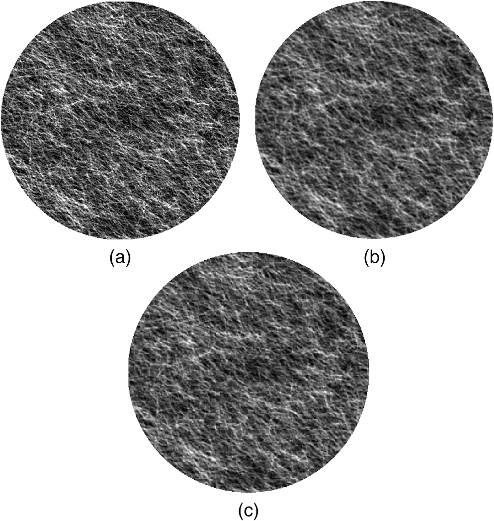

The second image was taken from a newsprint sample. In a printed newsprint, the text lines are known, a priori, to be in the cross direction, i.e., transverse to the direction of the main fiber orientation. The newsprint sample was rotated by 30 deg so that, in the image, the direction of main fiber orientation was at about 30 deg. No other prior knowledge about the orientation distribution was available. The newsprint image, taken through an optical microscope with a CCD camera, is shown in Fig. 5.

Fig. 5

(a) An optical-transmission (bright-field) image of a sample of newsprint. (b) A coarse-grained version of this image with smoothening. (c) A coarse-grained version of this image without smoothening.

The third image is that of organic nanofibrils taken with an atomic force microscope (AFM) (see Fig. 6). The size of the original square image was $512 \times 512 pixels$ , i.e., its diameter is 512 pixels (2 μm). Finally, the bright-field image of a paper sample shown in Fig. 1 was also analyzed.

Fig. 6

An atomic force microscope image of a thin film made of organic nanofibrils. (b) A coarse-grained version of this image with smoothening. (c) A coarse-grained version of this image without smoothening.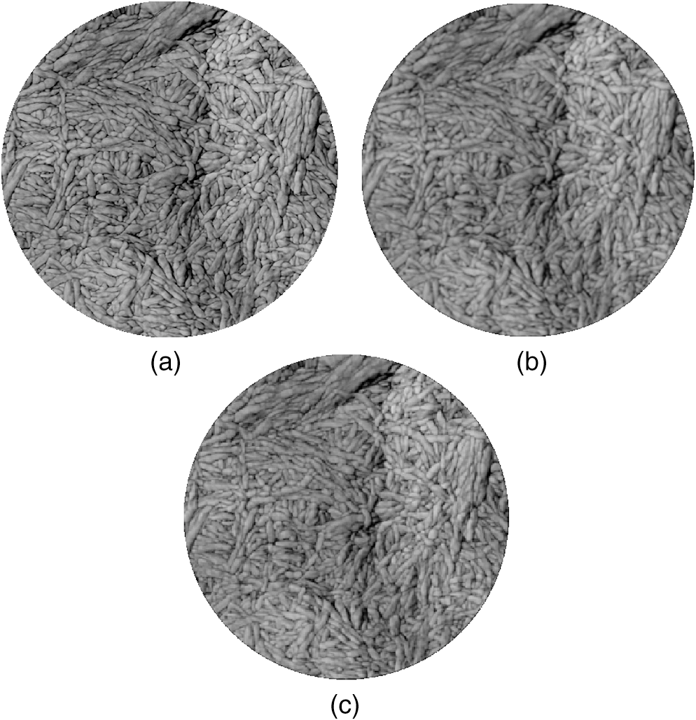

In order to test the performance of the above methods as a function of resolution, we also created two “corrupted” versions from the images described above. First, we downsampled the original image so as to have one fourth of the linear scale of the original image, i.e., from an image of $1024 \times 1024$ ( $512 \times 512$ for the nanofibrils case) pixels we created an image of $256 \times 256 pixels$ . Then, we rescaled it back to $1024 \times 1024 pixels$ without any interpolation and with a bilinear interpolation. This gave us two additional images, one where each pixel of the image was composed of $4 \times 4$ original pixels (without interpolation) and one where the new pixels were smoothed (with interpolation). The image without interpolation could be considered as one composed of rectangles: Its long edges were not straight but were composed of small vertical and horizontal pieces. On the other hand, the image with interpolation had smoothed edges.

4.2.

Reference Methods

As the first traditional method, we used a direct Fourier-analysis (FFT)-based method.¹ In this method, one simply computes the average of absolute values of the 2-D Fourier-transform coefficients of $f$ along radial lines. Similarly to our curvelet-based method, low frequencies are neglected in the analysis. We implemented this traditional method with small modifications: Instead of averages of absolute values, we used averages of their squares and instead of truncating off the two lowest frequencies we considered it more reasonable (based on simulations) to truncate off the 100 lowest frequencies.

The second traditional method was the so-called ST method,²^–⁵^,²⁵ i.e., one of the gradient methods developed recently. The ST tries to find a direction, $θ_{m}$ , in which the $L^{2}$ norm of the directional derivative is maximized. This method has three essential parameters: the size of the moving window that restricts the region considered at the time, the method used for a numerical estimation of gradients, and the thresholding value that removes the regions of weak orientation from the analysis. In our analysis, we used the ImageJ blug-in called OrientationJ.²⁵ In this application, the size of the moving window was set to minimum, the method used a for numerical estimation of gradients was the Gaussian-gradient method and no thresholds were used.

For both methods, the choice of the parameters was made so that estimation of the original simulated image looked as good as possible. Values of these parameters did not affect radically the duration of the analysis. The ST method is such that it gives an unlimited resolution for the angle parameter. For the FFT and curvelet methods, increasing of the angle resolution increases the duration of analysis, in principle linearly. However, in practice when the angle resolution was comparable to the image resolution, i.e., if about $N$ different angles were used for an image of $N \times N pixels$ , then the both curvelet and FFT-based methods were possible to implement with an about $N^{2} \log (N)$ scaling of efficiency. This was the amount of operations that the FFT took. Moreover, the implementation of a moving window in the ST method is often most efficient using the FFT, i.e., durations of analysis of these three methods were similar if their algorithms were optimized. In this work, the angle resolution was chosen to be one degree in all the methods. Also, a lower resolution would have given almost similar results: For the FFT and curvelet methods the results with a lower angular resolution would have been the same as for the corresponding subsamples of the results with a higher angular resolution. Of course, a reasonable lower limit for the resolution is difficult to know before any analysis, i.e., a resolution that is about the same as that of the image would be advisable if no prior knowledge about the problem is available.

The actual runtimes were measured with MATLAB^® R2010b using a few years old 64-bit computer with a 3.16-GHz Intel Core(TM)2 Duo processor and 4.00 GB of RAM memory. The actual runtimes (no algorithm was optimized) of the three codes (curvelet, FFT, and ST) for three different discretizations of Fig. 4 are shown in milliseconds in Table 1. It should be noted that using C or a more machine-related language and optimizing the codes for the real application, these runtimes could be reduced quite much, but they give anyway an idea of the relative performances of these methods. We know for sure that the algorithm based on the curvelet method at least could be made faster by one or two orders of magnitude, but such an optimization was beyond the scope of the present article, and was left for a future publication.

Table 1

Actual runtimes in milliseconds of the curvelet, fast Fourier transform (FFT), and structure tensor (ST) algorithm for three different discretizations (256×256, 512×512, and 1024×1024 pixels) of Fig. 4.

Method	Resolution
Method	$256 \times 256$	$512 \times 512$	$1024 \times 1024$
Curvelet	6.84	23.2	159
FFT	16.9	36.9	121
ST	207	809	3203

4.3.

Results and Discussion

Let us first compare the performance of the three methods in the orientation analysis of Fig. 1. In Fig. 7, we show the results of this analysis by the FFT (a), ST (b), and curvelet methods (c). Notice that the FFT distribution describes an orientation with multiple peaks, while the ST distribution has only one clear maximum. The curvelet distribution is in a sense an interpolation of the two. It is binomial with a global maximum at the same angle (a bit over 30 deg) as the ST distribution, and a side maximum at about $- 60 \deg$ . The anisotropies of these distributions are very small, however, so that this paper sample is almost isotropic.

Fig. 7

Estimations for distribution of fiber orientation of the paper sample of Fig. 1. Orientation distribution determined by the fast Fourier transform (FFT) method (a), the one determined by the structure tensor (ST) method (b), and the one determined by the curvelet method (c).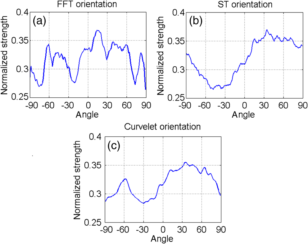

Comparison of the three estimates for the distribution of fiber orientation in the generated network of Fig. 4(a) against the known distribution makes it evident that the curvelet-based method gives somewhat better results than the other two methods (see Fig. 8). The curvelet method seems to estimate the overall distribution quite well and to locate the maximum very accurately. Notice that the ST method clearly overestimates the orientation strength. Use of other parameters in the ST method could result in a considerably worse distribution. The distribution of the FFT method is close to that of the curvelet-based method, however, it underestimates a little the known distribution.

Fig. 8

Estimations for distribution of fiber orientation in the image of a numerically generated network of fibers shown in Fig. 4(a). Orientation distribution as determined by the FFT method (upper left panel), the one determined by the ST method (upper right panel), and the one determined by the curvelet method (lowest panel). Each panel includes also the known orientation distribution (the dashed lines) for comparison.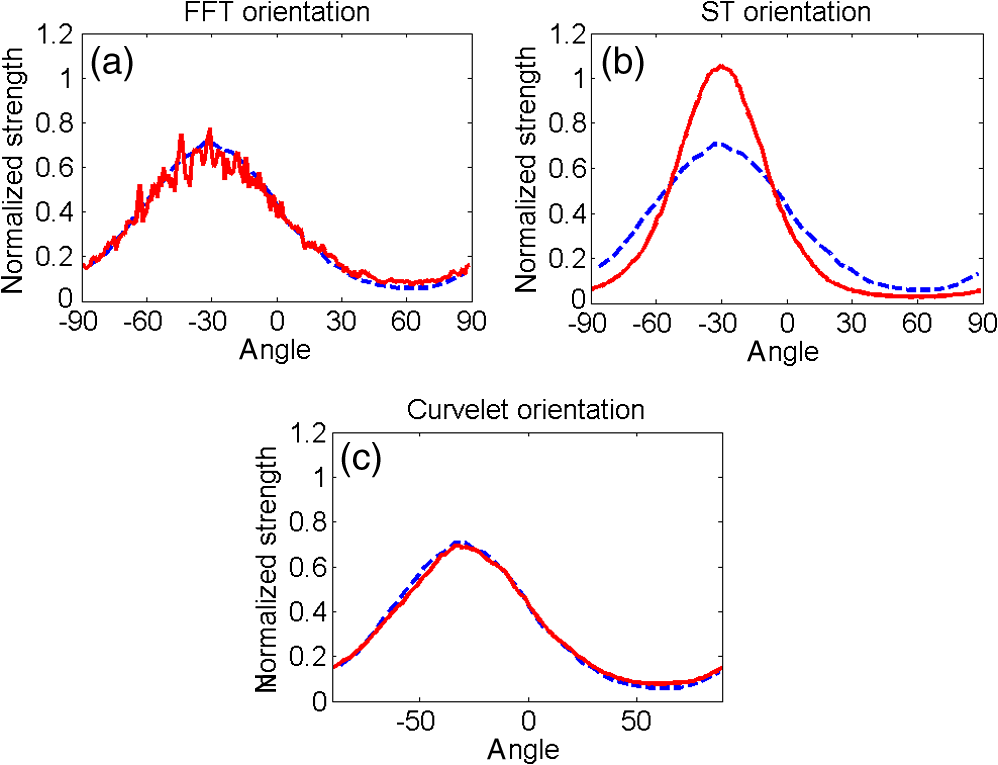

In Figs. 9 Fig. 10 to 11, we test the robustness of the three methods by applying them to the coarse-grained versions of the original image of the computer-generated network. It is evident from Fig. 9 that the curvelet-based method is very robust against coarse graining. As could be expected, Fig. 10 provides evidence for a failure of the FFT method to deal with the nonsmoothed coarse-grained image (no interpolation). Also, the orientation estimate for the smoothed coarse-grained image (with interpolation) is quite poor. Figure 11 demonstrates that also the ST method gives a poor result for the nonsmoothed coarse-grained image. However, quite unexpectedly, for the smoothed coarse-grained image, the result of the ST method is better than for the original image.

Fig. 9

Curvelet-based estimates for the distribution of fiber orientation as determined from the original generated network of Fig. 4(a) and its two coarse-grained versions (as explained in the text).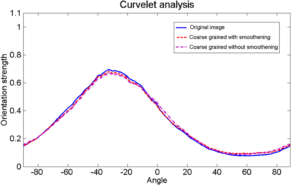

Fig. 10

FFT-based estimates for the distribution of fiber orientation as determined from the original generated network of Fig. 4(a) and its two coarse-grained versions (as explained in the text).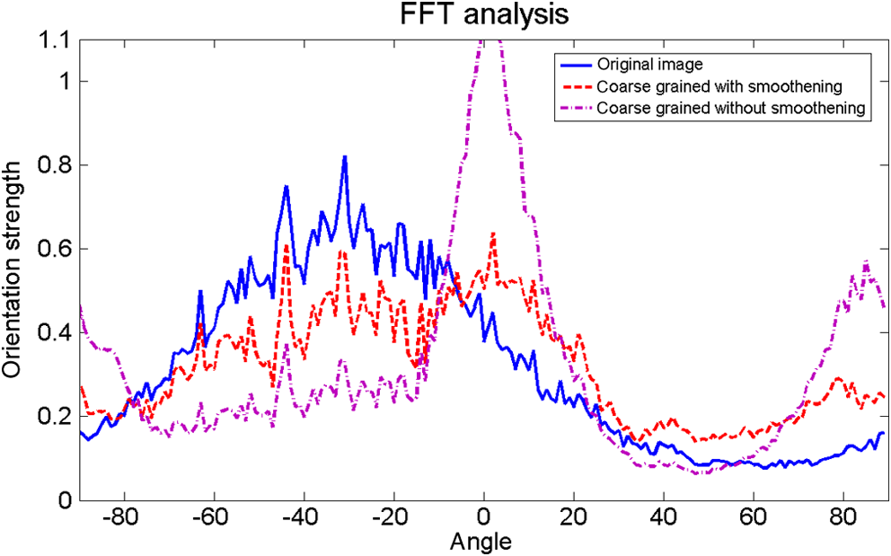

Fig. 11

ST-based estimates for the distribution of fiber orientation as determined from the original generated network of Fig. 4(a) and its two coarse-grained versions (as explained in the text).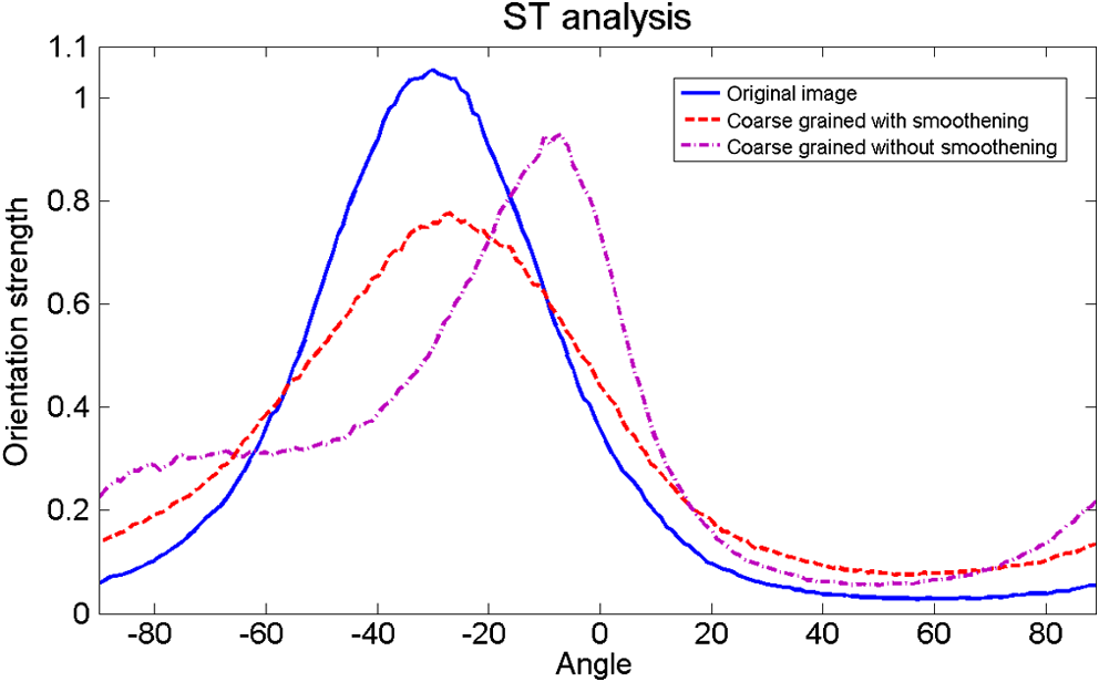

Similar comparisons are made in Figs. 12 Fig. 13 to 14 for the newsprint sample of Fig. 5(a), and for two coarse-grained versions (as above) of it.

Fig. 12

Curvelet-based estimates for the distribution of fiber orientation of the original newsprint sample [Fig. 5(a)] and its two coarse-grained versions.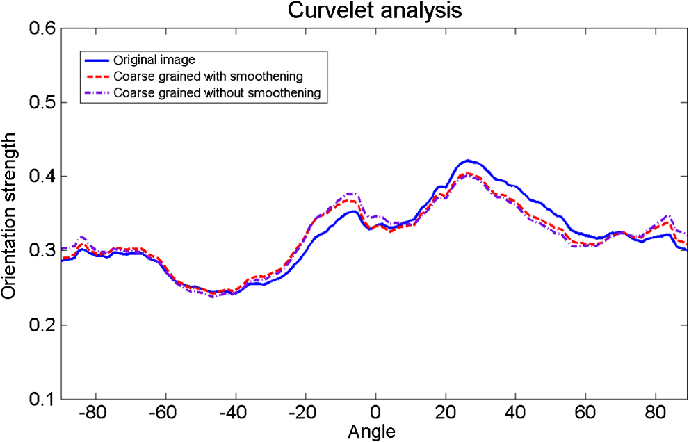

Fig. 13

FFT-based estimates for the distribution of fiber orientation of the original newsprint sample [Fig. 5(a)] and its two coarse-grained versions.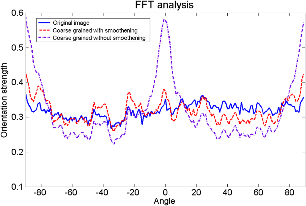

Fig. 14

ST-based estimates for the distribution of fiber orientation of the original newsprint sample [Fig. 5(a)] and its two coarse-grained versions.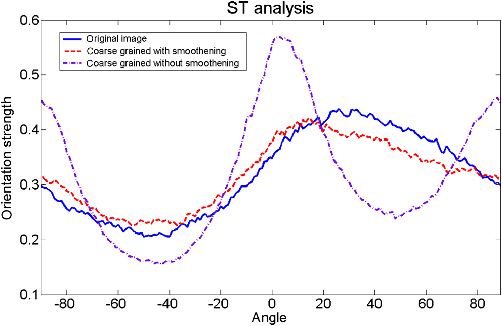

It is evident from these figures that only the curvelet method has the maximum in the orientation distribution at the correct position independent of coarse graining of the image. In fact, this method seems to produce very similar distributions in all three cases, see Fig. 12, while the FFT method seems to fail in all these cases, also for the original image (Fig. 13). The ST method works quite well for the original newsprint sample (see Fig. 14). It fails to give a reasonable estimate for the nonsmoothed coarse-grained image, however.

Comparison of the orientation-distribution estimates for the nanofibrer image (Fig. 9) is more difficult since there is no prior knowledge of the actual distribution.

It is evident from Fig. 15 that the curvelet method is not so robust as before (fiber networks) for this type of image: the main peak and side peak seem to change their roles in the analysis of the original and coarse-graind images, respectively. The reason for this may be the bundles of nanofibers (e.g., in the upper part of the image) that begin to dominate the coarse-grained images. Also, nanofibers are not so elongated than the fibers in the two previous applications (see Figs. 4 and 5), and parameters of the curvelet method may need to be tuned differently for this particular case.

Fig. 15

Curvelet-based estimates for the distribution of fiber orientation of the original nanofiber image [Fig. 6(a)] and its two coarse-grained versions.

Figure 16 indicates that the FFT method does not produce very much of a clear structure for the original nanofiber image apart from the main orientation direction at about 0 deg. For the coarse-grained versions of the image, it gives an additional peak at about 90 deg, which obviously follows from coarse graining only and is thus an artifact. This method does not seem to tolerate coarse graining without smoothening. The ST method seems to find for the original image a very broad and flat peak in the range of angles, where the curvelet method finds two-local maxima. For the image coarse-grained with smoothening (see Fig. 17), it seems to find the same side peak as the curvelet method, however. In this case, the ST method seems to work for the smoothed coarse-grained image better than for the original image. For the nonsmoothed coarse-grained image the ST method clearly fails. Overall, the orientation distribution of the nanofibrer image seems to be difficult to estimate, and it also demonstrates that a method optimized for one type of image does not necessarily work as well for another type of image.

Fig. 16

FFT-based estimates for the distribution of fiber orientation of the original nanofiber image [Fig. 6(a)] and its two coarse-grained versions.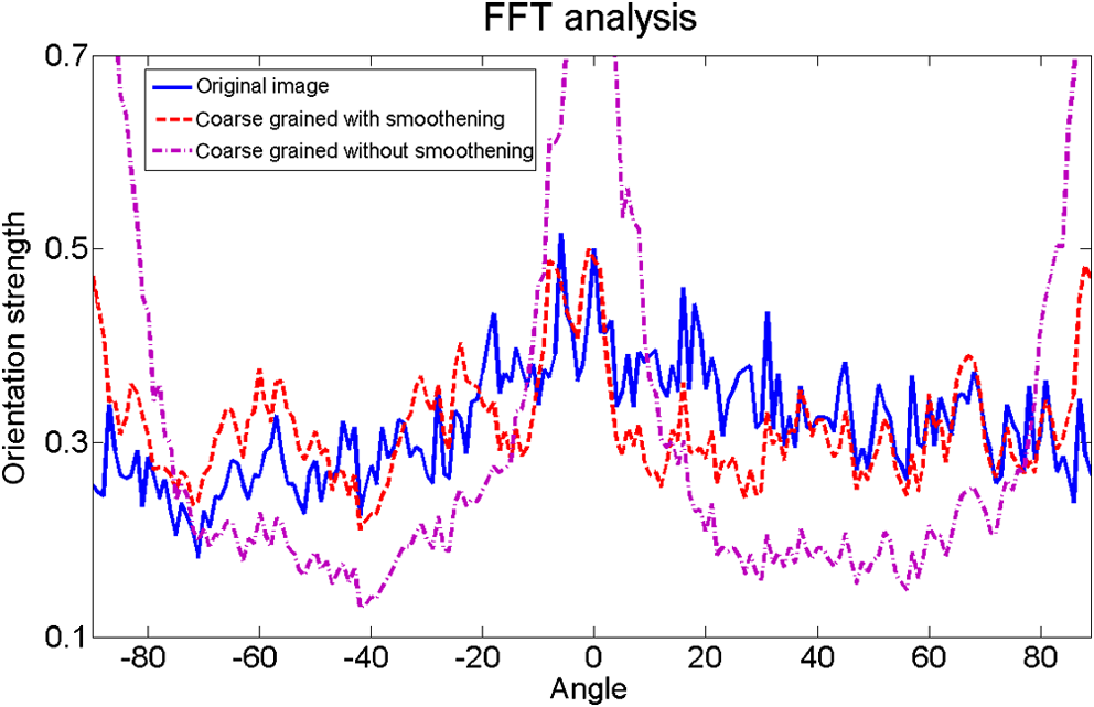

Fig. 17

ST-based estimates for the distribution of fiber orientation of the original nanofiber image [Fig. 6(a)] and its two coarse-grained versions.

5. Conclusions

A new method based on the curvelet transform was introduced for estimating the distribution of orientation in images of elongated features (particles). The mathematical justification of the suitability of the method for this kind of application was briefly demonstrated.

The known distribution of orientation in the computer-generated network of fibers was accurately produced by this method. Furthermore, this method was applied to two optical images of fibrous samples (paper), an AFM image of a membrane of nanofibers, and two of their (differently) coarse-grained versions, with good results even though the AFM image was quite challenging. The performance of this method was also compared with those of two traditionally used methods of orientation analysis, i.e., the FFT- and ST-based methods. The curvelet method was demonstrated to be more accurate and stable than these other two methods, and it was shown in particular to be more robust against coarse graining of the image. This means that the curvelet method gives more reliable results when the resolution of the image is low.

Acknowledgments

This work was supported financially by ForestCluster Ltd. (projects Qvision and EffNet). Moreover, the work was supported in part by the Academy of Finland (projects 141094, 255891, and 255824).

References

1.

T. EnomaeY.-H. HanA. Isogai, “Nondestructive determination of fiber orientation distribution of paper surface by image analysis,” Nord. Pulp Pap. Res. J., 21 (2), 253 –259 (2006). http://dx.doi.org/10.3183/NPPRJ-2006-21-02-p253-259 NPPJEG 0283-2631 Google Scholar

2.

T. Broxet al., “Adaptive structure tensors and their applications,” Visualization and Processing of Tensor Fields, 17 –47 Springer-Verlag, Berlin (2006). Google Scholar

3.

R. van den BoomgaardJ. van de Weijer, “Robust estimation of orientation for texture analysis,” in Second Int. Workshop Texture Anal. Synth., (2002). Google Scholar

4.

S. K. NathK. Palaniappan, “Adaptive robust structure tensors for orientation estimation and image segmentation,” Lect. Notes Comput. Sci., 3804 445 –453 (2005). http://dx.doi.org/10.1007/11595755 LNCSD9 0302-9743 Google Scholar

5.

M. Krauseet al., “Determination of the fibre orientation in composites using the structure tensor and local x-ray transform,” J. Mater. Sci., 45 888 –896 (2010). http://dx.doi.org/10.1007/s10853-009-4016-4 JMTSAS 0022-2461 Google Scholar

6.

I. Daubechies, Ten Lectures on Wavelets, Society for Industrial and Applied Mathematics (SIAM), Philadelphia, Pennsylvania (1992). Google Scholar

7.

E. J. CandèsD. L. Donoho, “Recovering edges in ill-posed inverse problems: optimality of curvelet frames,” Ann. Stat., 30 (3), 784 –842 (2002). http://dx.doi.org/10.1214/aos/1028674842 ASTSC7 0090-5364 Google Scholar

8.

E. J. CandèsD. L. Donoho, “New tight frames of curvelets and optimal representations of objects with piecewise C2 singularities,” Commun. Pure Appl. Math., 57 (2), 219 –266 (2004). http://dx.doi.org/10.1002/(ISSN)1097-0312 CPMAMV 0010-3640 Google Scholar

9.

M. N. DoM. Vetterli, “The contourlet transform: an efficient directional multiresolution image representation,” IEEE Trans. Image Process., 14 (12), 2091 –2106 (2005). http://dx.doi.org/10.1109/TIP.2005.859376 IIPRE4 1057-7149 Google Scholar

10.

K. GuoD. Labate, “Optimally sparse multidimensional representation using shearlets,” SIAM J. Math. Anal., 39 (1), 298 –318 (2007). http://dx.doi.org/10.1137/060649781 SJMAAH 0036-1410 Google Scholar

11.

O. Wirjadiet al., “Applications of anisotropic image filters for computing 2D- and 3D-fiber orientations,” 107 –112 2009). Google Scholar

12.

C. SöremarkG. JohanssonA. Kiviranta, “Characterization and elimination of fiber orientation streaks,” in Tappi Eng. Conf., 97 –104 (1994). Google Scholar

13.

A. KivirantaP. Pakarinen, “New insight into fiber orientation streaks,” in TAPPI Papermakers Conf. Proc., 7 (2012). Google Scholar

14.

K. Niskanen, “Paper physics,” Papermaking Science and Technology, Fapet, Jyväskylä (1998). Google Scholar

15.

T. Uesakaet al., “Curl in paper: derivation of approximate curl formulae and their applicability,” Jpn. Tappi, 41 (4), 335 –341 (1987). http://dx.doi.org/10.2524/jtappij.41.335 0022-815X Google Scholar

16.

U. HirnW. Bauer, “Investigating paper curl by sheet splitting,” 2006). Google Scholar

17.

C. Antoineet al., “3D images of paper obtained by phase-contrast X-ray microtomography: image quality and binarisation,” Nucl. Instrum. Methods Phys. Res. Sect. A, 490 (1–2), 392 –402 (2002). http://dx.doi.org/10.1016/S0168-9002(02)01003-3 0168-9002 Google Scholar

18.

E. J. CandèsD. L. Donoho, “Continuous curvelet transform. I: resolution of the wavefront set,” Appl. Comput. Harmon. Anal., 19 (2), 162 –197 (2005). http://dx.doi.org/10.1016/j.acha.2005.02.003 ACOHE9 1063-5203 Google Scholar

19.

E. J. CandèsD. L. Donoho, “Continuous curvelet transform. II: Discretization and frames,” Appl. Comput. Harmon. Anal., 19 (2), 198 –222 (2005). http://dx.doi.org/10.1016/j.acha.2005.02.004 ACOHE9 1063-5203 Google Scholar

20.

J. SampoS. Sumetkijakan, “Estimations of Hölder regularities and direction of singularity by Hart Smith and curvelet transforms,” J. Fourier Anal. Appl., 15 (1), 58 –79 (2009). http://dx.doi.org/10.1007/s00041-008-9054-9 1069-5869 Google Scholar

21.

V. BrytikM. V. de HoopM. Salo, “Sensitivity analysis of wave-equation tomography: a multi-scale approach,” J. Fourier Anal. Appl., 16 (4), 544 –589 (2010). http://dx.doi.org/10.1007/s00041-009-9113-x 1069-5869 Google Scholar

22.

J. Sampo, “On convergence of transforms based on parabolic scaling,” Lappeenranta University of Technology, (2010). http://urn.fi/URN:ISBN:978-952-265-026-9 Google Scholar

23.

E. J. CandèsD. L. DonohoL. Ying, “CurveLab Toolbox,” http://www.curvelet.org/software.html Google Scholar

24.

A. Ekmanet al., “The number of contacts in a random fiber networks,” Nord. Pulp Pap. Res. J., 27 270 –276 (2012). http://dx.doi.org/10.3183/NPPRJ-2012-27-02-p270-276 NPPJEG 0283-2631 Google Scholar

25.

R. Rezakhanihaet al., “Experimental investigation of collagen waviness and orientation in the arterial adventitia using confocal laser scanning microscopy,” Biomech. Model. Mechanobiol., 11 (3–4), 461 –473 (2012). http://dx.doi.org/10.1007/s10237-011-0325-z BMMICD 1617-7959 Google Scholar

Biographies of the authors are not available.

CC BY: © The Authors. Published by SPIE under a Creative Commons Attribution 4.0 Unported License. Distribution or reproduction of this work in whole or in part requires full attribution of the original publication, including its DOI.

Citation Download Citation

Jouni A. Sampo, Jouni J. Takalo, Samuli Siltanen, Arttu Miettinen, Matti Lassas, and Jussi Timonen "Curvelet-based method for orientation estimation of particles from optical images," Optical Engineering 53(3), 033109 (27 March 2014). https://doi.org/10.1117/1.OE.53.3.033109

Published: 27 March 2014

Access the abstract

JOURNAL ARTICLE
11 PAGES

DOWNLOAD PAPER SAVE TO MY LIBRARY

GET CITATION

CITATIONS

Cited by 7 scholarly publications.

Explore citations on Lens.org

KEYWORDS

Optical fibers

Particles

Calcium

Statistical analysis

Optical engineering

Image resolution

Nanofibers

1.

Introduction

2.

Optical Imaging of Fibers

Fig. 1

Fig. 2

3.

Mathematical Methods

3.1.

Curvelet Transform

Eq. (1)

Eq. (2)

Fig. 3

Eq. (3)

Eq. (4)

3.2.

Decay of the Transform

Theorem 3.1.

Eq. (5)

Theorem 3.2.

Eq. (6)

Proof of Theorem 3.2

3.3.

Estimate for the Distribution of Particle Orientations

Eq. (7)

Eq. (8)

Eq. (9)

4.

Comparison with Other Methods

4.1.

Test Images

Fig. 4

Fig. 5

Fig. 6

4.2.

Reference Methods

Table 1

4.3.

Results and Discussion

Fig. 7

Fig. 8

Fig. 9

Fig. 10

Fig. 11

Fig. 12

Fig. 13

Fig. 14

Fig. 15

Fig. 16

Fig. 17

5.

Conclusions

Acknowledgments

References

Show All Keywords

Keywords/Phrases

Search In:

Publication Years