|
|
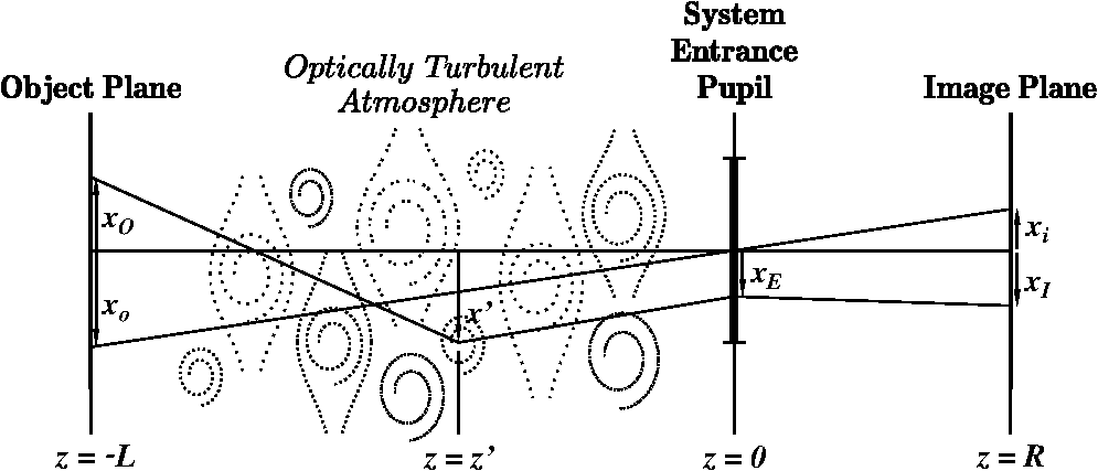
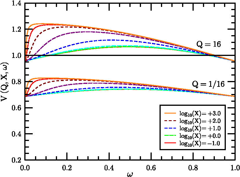
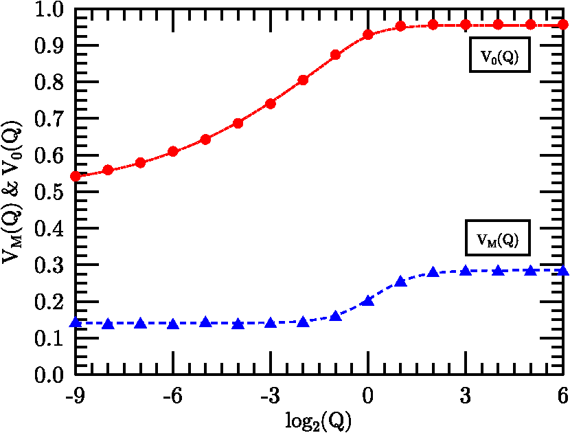
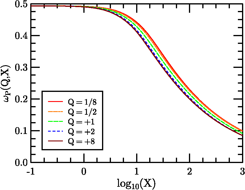
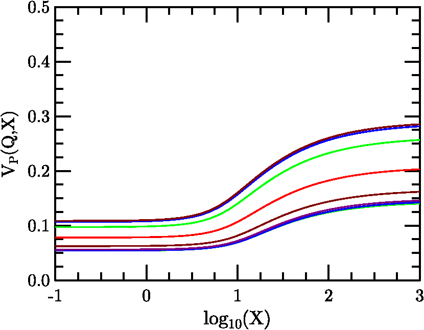
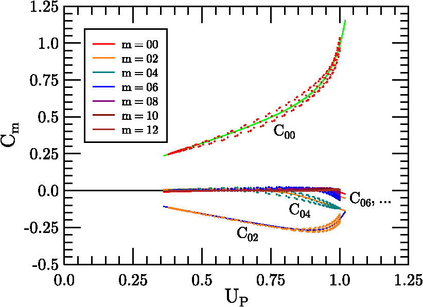
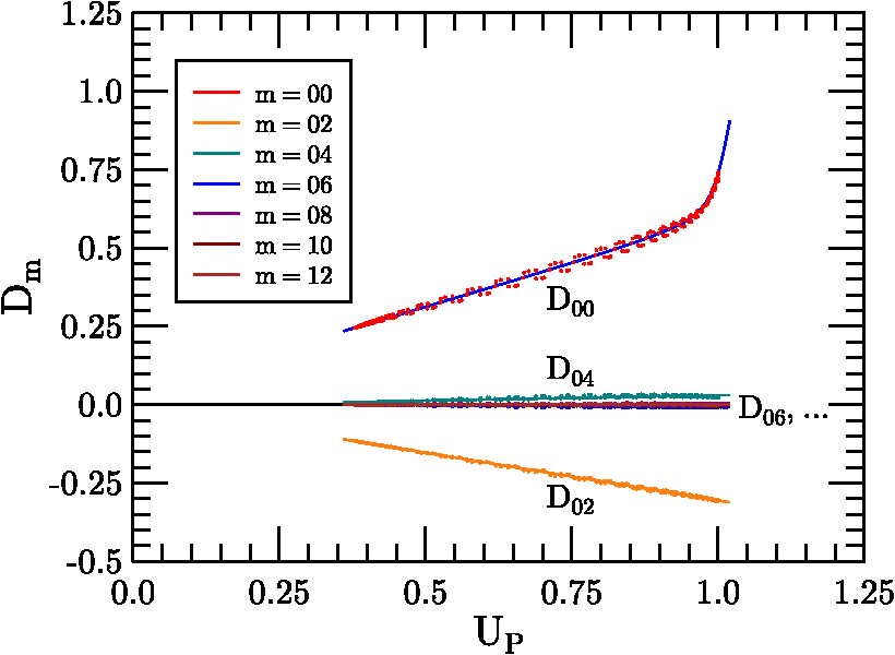
1.IntroductionThe problem of imaging in the presence of degrading optical turbulence conditions has been an ongoing area of active research for many years. Much recent research has focused on correcting imagery through image processing (dewarping and/or deconvolution) techniques.1–8 Paralleling this inverse problem is the direct simulation of turbulence on clear images to create artificially degraded imagery at known turbulence levels9–12 for benchmarking purposes. A third research area involves system intercomparisons for cost-effectiveness evaluation.13–15 In each case, undergirding the research is the core issue of establishing the baseline effect of turbulence on image quality, particularly for short-exposure (SE) imaging. The standard method used by systems performance modelers13–17 had been Fried’s SE modulation transfer function (MTF).18–20 For example, Holst15 devotes an entire chapter to Fried’s SE MTF. This model was the common choice due to its simplicity, despite the existence of more accurate (and numerically intensive) techniques (e.g., Ref. 21). Critics of Fried’s approach pointed to its high-frequency response failure when modeling high turbulence degradation influences.21–23 Nonetheless, the simplicity of Fried’s result suggested a re-examination of Fried’s approach might yield new findings. The resulting study24 examined the properties of an overlooked tilt-phase correlation term and developed improved expressions for diffraction influences on the turbulent phase structure function (PSF), angle-of-arrival variance, and therefore on the SE MTF. However, the numerical integration technique used was not optimal for evaluating the tilt-phase influence at combined high-angular frequency and high-turbulence conditions. Consequently, a modeling compromise was adopted based on Fried’s quadratic correction to the long-exposure (LE) MTF. This approach was subsequently critiqued by Charnotskii25–28 who argued its quadratic term would produce inaccurate results at high frequency. This issue is addressed here through a new analysis of high-frequency turbulence effects and development of a new SE MTF analytic model. The new model exhibits diffraction-limited behavior at all frequencies while applying to a wider range of optical scenarios. The resulting model is compared with published calculations from a path-integral technique21 and a Markov method.26 The model’s Rytov approximation (RA)29 is also described, and criteria developed by Tatarski29 and Dashen30 are examined to determine the extent of validity of modeled conditions. The remainder of the paper is designed as follows: Section 2 describes the propagation model used, its justification, and numerical processing techniques developed to handle high-turbulence conditions. Section 3 describes the analysis process used to translate the computed database into the new analytical SE MTF expression. Section 4 presents comparisons with alternative approaches, followed by conclusions in Sec. 5. 2.Propagation and Imaging ModelsThe propagation model used is based on the Rytov approximation,16,29 involving a multiplicative turbulent scattering effect, using the imaging geometry of Fig. 1. Monochromatic incoherent light of wavelength emerges from the transverse object plane at . Photons pass through the system aperture’s lens at to reach the imaging plane at . The system’s thin lens optics are considered focused on the object plane. The main propagation axis is denoted by ; transverse two dimensional (2-D) vectors are denoted by . In general, light from a point is evaluated for scatter off the ensemble of turbulent fluctuations at , passage through the aperture at and its effect on the light at image point . Each object point will have a reciprocal image point at following a chief ray through the center of the system entrance pupil. Due to the incoherent nature of the light, each photon travels independently, emitted as a quantum event, and arriving at the image plane based on conditional passage through the system entrance pupil. The instantaneous point spread function represents the electro-magnetic equivalent of the photon’s quantum probability of arrival at image point , given the current optical turbulence pattern (considered frozen) in the region . 2.1.Propagation ModelThe Rytov approximation considers a propagating scalar wavefunction consisting of a zeroth-order free-space solution, , plus a complex turbulence multiplier. contains the primary longitudinal phasor , where and is the wavenumber, plus the phase information necessary to determine the zero-turbulence focal point of the source point in the image plane, and spherical wave phase information that will be focused by the system lens effect.Turbulent amplitude () and phase () effects are imposed on the propagating wave via weak scattering from position-varying refractive index fluctuations where is the expectation (mean) of the refractive index . Turbulent fluctuations will be modeled (exceptions noted) assuming Kolmogorov turbulence, characterized by the power spectrum26 where is the turbulent spatial frequency . For natural turbulence, , such that the refractive index structure parameter, , is typically less than , leading to forward scattering (in the direction), and use of the parabolic wave equation with the on-axis derivative operator, and the transverse Laplacian.Using Eq. (1)’s model propagating wave, the RA method’s single-scattering approximation is used to evaluate and instantaneous amplitude and phase perturbations for radiation emerging from a source at at system entrance pupil points, , This equation reflects scattering from turbulence at points , , using free-space Green’s function propagators16 with and , to propagate the field from the source, through the scattering point, to the observation point. The Green’s function in the denominator normalizes the results according to the free space effect. Note, particularly, that and are source and observation point dependent quantities; therefore they are anisoplanatic.2.2.Modulation Transfer FunctionFollowing the methodology of Ref. 24, we analyze the wave perturbations at the system’s entrance pupil associated with the instantaneous SE MTF for the source point Here, the field variables reflect the situation just after truncation by the aperture and have had the mean wavefront tilt and curvature removed. The system entrance pupil is modeled using a uniformly transparent window functionAccording to Fried’s SE theory, the instantaneous turbulent phase tilt is removed, based on variable denoting the linear moment of the instantaneous phase perturbation Vector variable is a normalized angular frequency, where denotes the diffraction-limited maximum angular frequency16 passed by a circular aperture, such that . is the entrance pupil diameter, dimensionalizing temporarily, before is used to transform integral (10) to dimensionless form. The mean SE MTF sought is then evaluated by taking the expectation of Eq. (7), and where the turbulent effects are expressed as the terms. The expectation operator was passed inside the integral, as it affects only the turbulence terms. It is worth noting that this averaging process transforms the anisoplanatic instantaneous MTF into an isoplanatic second-order function, consistent with Goodman’s16 analysis (pp. 395–407).For brevity of presention, only results are shown here, based on more complete descriptions in Refs. 20 and 24. First, amplitude and phase perturbations are considered independent, permitting the expectation of the amplitude term to be evaluated as using , the amplitude structure function.31 The remaining three terms are phase related, involving phase variance, tilt variance, and tilt-phase terms. The second term is the phase variance term, appearing as where is the PSF. This term combines with to form the wave structure function (WSF), , shown in path-integral form as Eq. (11) of Ref. 24. This combined term quantifies the turbulence LE effect. While the instantaneous perturbation effects were source specific (), therefore anisoplanatic, satisfying an energy conservation constraint,32 the second-order WSF is source independent, evaluated by weighted path integral of ,31 therefore isoplanatic.Assuming constant Kolmogorov turbulence throughout the following with , using the Fried coherence diameter20,24The remaining two terms reflect SE corrections to the LE MTF (due to ). The tilt variance term that can be written24 introducing parameter to characterize diffraction influences, and function that varies from to 1; for ( plotted in Ref. 24).Since , , and are independent of , they do not affect the aperture integral of Eq. (11). The remaining tilt-phase correlation, written 24 must be evaluated numerically. An improved version of the PSF model is introduced to facilitate evaluation of where is a normalized separation variable, and have absorbed the factors, and parameterizes the diffraction influence24 using dimensionless path () and frequency () variables. Function transitions from to 1 over eight orders of magnitude in .24When turbulence is low (), the turbulent exponential argument approaches zero, and the SE MTF approaches the behavior of the system MTF, which depends only on , due to azimuthal symmetry.When , the Eq. (11) integral was evaluated numerically using the form where the system MTF, a function independent of and , could be divided out to focus on the turbulence-varying component. In the prequel,24 evaluation of was handled using a relatively inefficient integration technique, but here, based on the PSF of Eq. (18), was removed from the exponential integral, allowing the remaining term to be tabulated and used for interpolation. The dimensionality of the tabulated results was also reduced through application of azimuthal symmetry that permitted the orientation of to be fixed along the -axis (unit vector, ).Third, the evaluations were modified to handle the impact of large effects inside the exponential through use of an offset factor By adjusting , math overflow errors in evaluating the integral could always be eliminated. Thereafter, calculations could be interpreted in the form Combining this term with the tilt variance effect of Eq. (16) yields the function such that the SE MTF can be writtenCalculations of the function were performed for a wide range of conditions: from to by factors of 2 (9 steps), from to in increments of tenths of decades (41 steps), and from 0.01 to 0.99 in steps of 0.01, and four additional steps at (103 steps), for a database of 38,007 calculations. The analysis of this database is described in Sec. 3, using these results to formulate a new analytic SE MTF. Sections 5 through 7 of Ref. 24 provides further details of the analysis of Fried’s approach. 2.3.Range of Rytov Approximation ValidityBefore examining the database, some discussion of the extent of validity of the Rytov method seems appropriate. Clearly, the Rytov approximation is applicable to coherent radiation studies under weak turbulence conditions, but is typically considered inappropriate for stronger turbulence scenarios, when the Rytov variance exceeds 0.5 (spherical wave coefficient used). However, in light of subsequent comparisons with Charnotskii’s results21,26 in Sec. 4, where comparable results are achieved at Rytov variance values seemingly beyond the capability of the RA, one may question the validity of such restrictions for incoherent radiation, since temporal and spatial correlations do not exist between propagating photons.Tatarski’s analysis29 only required that , and that perturbation field gradients be small relative to wave number , conditions easily met. Similarly, Dashen30 developed full and partial saturation conditions for judging RA validity, formed as ratios of a turbulence parameter, , to a diffraction parameter, . For the full saturation case, Dashen used, where models a single scatterer scale. For a turbulent outer scale of , and a spectral model33 based on Kaimal’s 1968 Kansas experiment analysis,34 . For the turbulence parameter, Dashen used a phase variance metric also based on an outer-scale influenced covariance In this case, the RA is valid when , or, easily met for common outer scales of 1 m or greater.More stringent conditions were associated with a partial saturation case involving multiple scattering scales. Dashen considered the effect of imposing a scale size cutoff that would affect both turbulent and diffraction effects. For the SE imaging problem, the most natural cutoff is the finite aperture. Dashen’s , corresponding to an RMS phase variance, is equivalent to one of Fried’s18 mean aperture phase variance terms, where the order indicates the number of phase perturbation terms corrected during the imaging process. In SE imaging, piston, tip, and tilt phase-expansion terms do not alter image quality (corresponding to Fried’s order-L case), leading to the condition, for an aperture of diameter . For cutoff , Dashen’s parameter becomesSetting , for a given , a maximum value results This condition translates to a maximum Rytov variance function of Typical terrestrial imaging scenarios involve , implying the RA remains valid up to high-turbulence conditions. 3.Analytic Model of Short-Exposure Atmospheric Modulation Transfer FunctionUsing the previous section’s data set, this section describes development of an analytic expression for . This is possible due to significant correlations that exist between results at different values. This behavior is illustrated in Fig. 2 for two sets of plots at values of and 16, for a series of increasing values of . The key feature of these curves is that for moderate values often encountered for typical terrestrial imaging scenarios, exceeds unity at low to moderate frequencies, resulting in enhanced behavior versus the LE response. In developing a model of this behavior, it was first observed that , permitting to be expressed The maximum value of (as ) must also be a function of , . and are plotted in Fig. 3. Figure 3 curves both suggest asymptotic behaviors at both extremes of . These behaviors can be modeled using a sigmoidal function (a variant of the hyperbolic tangent) To facilitate the modeling process, a rescaled and shifted sigmoid was also introduced The center of this function occurs at with an overall shift of between asymptotes, and a central derivative of . The function can be expressed using as However, exhibits different asymptotic behaviors at large and small . Therefore, a third sigmoidal form was developed, featuring a central splice (piecewise sigmoidal): This function is continuous in its first derivative at the splice point if . is parameterized using this function via where . Equations (39) and (41) are plotted along with database derived points in Fig. 3. Variables and will frequently appear hereafter as surrogates for variables and in arguments to sigmoidal functions, as the majority of the modeled behaviors exhibit logarithmic dependence.Using Eqs. (39) and (41), our problem reduces to finding an analytic expression for Figure 4 illustrates plots of for the same families of curves ( and 16) as in Fig. 2, highlighting the similarities in behaviors at different values. These plots also reveal how develops increasingly complex behaviors as increases. To model these behaviors, it was observed that function curves at high maintained simpler forms with increasing than at low , suggesting the functions could be divided at the peak and studied separately at high and low frequencies. The next step was, therefore, to model the form of the peak curves (as illustrated in Fig. 4) as functions of and . Note that the peak curves at different values exhibit similar dependencies. Thus, the behaviors of the different peak curves could be modeled as shifted versions of the peak curve for , described by (abscissa) and (ordinate) functions. The abscissa curve is modeled as Several curves at different levels illustrate this shifting behavior in Fig. 5. A pair of analytic expressions that approximate this behavior are given by Several ordinate function curves, designated (using the non-normalized form), are illustrated for varying in Fig. 6, for values ranging from to 16. This component exhibits both shifting and scaling properties, but again was quantified relative to its behavior at , using The behavior at was then rescaled using , and shifted using , in the form, The function supports a further parameterization through introduction of using Eqs. (47) and (39), where . The curve shapes appear to vary based on height , while dependence may be modeled using a Legendre-polynomial-related series expansion.The Legendre polynomials begin as , , and use recurrence relation35 to characterize the interval . Rescaling and normalizing these functions using where , yields an orthonormal set over .Using this basis set, each curve could be separated into two functions at the peak position , followed by affine transformation to stretch each monotonic function into its own half-range, and reverse copied to fill the opposing half-range. Thereby, two functions, each even about , could be analyzed using Legendre-derived basis functions. Due to their symmetry, only even-order series terms were needed to characterize each function . The model could, thus, be splined using the coefficient sets: for , and for , as Sets of coefficient behaviors are illustrated in Fig. 7. behaviors are plotted in Fig. 8. Coefficients through , and , exhibit approximately hyperbolic dependence. The remaining coefficients exhibit approximately linear dependence. Hyperbolic behaviors of and coefficients were expressed using constants through in the models Linear cases were modeled by setting . The curves plotted in Figs. 7 and 8 represent functional fits to computed values. Fit coefficients are listed in Tables 1 and 2. Table 1SPGD hyperbolic Cm and Dm coefficients.
Table 2SPGD linear Cm and Dm coefficients.
With the development of the and functional forms, the new analytic SE MTF model form was completed. However, given the number of free constants (80) involved, an open question remained whether a slightly modified set of coefficients could produce a better fit. To explore this possibility, a stochastic parallel gradient descent (SPGD) procedure36 was applied to improve the fit to the database. The coefficient set derived in the initial analysis (described above) was used to “seed” the SPGD optimizer. The SPGD consisted of randomly perturbing the full 80-parameter coefficient set, recomputing the RMS error for the full database, and comparing that error with the previous best fit error. Any new set that outperformed the prior best fit was adopted as the new best fit. Use of the SPGD reduced the overall RMS error of from 0.006795 to 0.002728. For simplicity of presentation, coefficients listed in Tables 1 and 2 represent the SPGD best-fit coefficients. For the remaining expressions, the original results (used in the plotted figures) were retained in Eqs. (39) through (49), so curves in the various figures can be replicated. Optimized versions of these equations are given below. To summarize, the new SE MTF model is formulated starting with the general expression in Eq. (27), then using from (20), from (36), from (42), expressions in Eqs. (44), (47), and (50) through (55), and results of the SPGD analysis 4.Comparisons with Alternative ApproachesThe analytic model developed in the previous section is compared here with results obtained by Charnotskii21,26 and several prior analytic methods. Charnotskii21 used a Feynmann-path integral technique. Figures 9 through 11 intercompare the new model with Charnotskii’s21 Figs. 8 through 10. Charnotskii’s parameter is related to via , such that values 0, , , , and correspond to values 0.000, 1.241, 2.851, 4.638, and 6.550, respectively. Charnotskii’s parameter is related to as . Reported values of the three plots were 10.0, 1.0, and 0.1, respectively, corresponding to values 2.523, 0.798, and 0.252. The curves (the uppermost line in each graph) correspond to the system MTF, and match identically. Remaining lines in Figs. 9 and 11 were plotted using values that produced the closest fit to Charnotskii’s results, in Fig. 9 and in Fig. 11. Lines in Fig. 10 were constructed based on the reported (). Systematic deviations employed in these plots appear consistent with Charnotskii comments that and constituted limiting cases, but might be due to approximations used when Charnotskii developed Eq. (31) of Ref. 21. Fig. 9Comparison of SE (solid lines) and LE (dashed lines) MTF model results using versus data (symbols) digitized from Ref. 21’s Fig. 8. 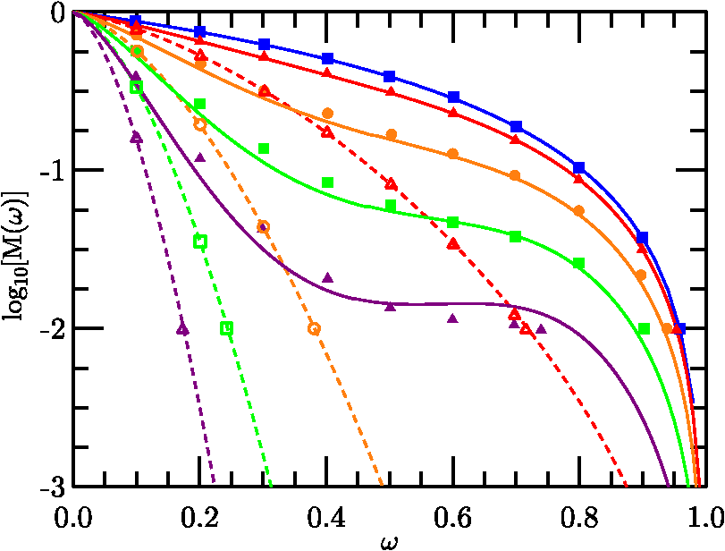 Fig. 10Comparison of SE (solid lines) and LE (dashed lines) MTF model results using versus data (symbols) digitized from Ref. 21’s Fig. 9. 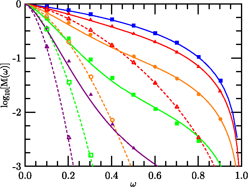 Fig. 11Comparison of SE (solid lines) and LE (dashed lines) MTF model results using versus data (symbols) digitized from Ref. 21’s Fig. 10. 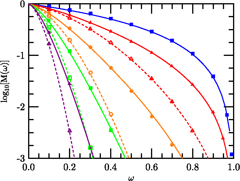 The comparisons of Figs. 9Fig. 10–11 provide partial verifications of both the present method and Charnotskii’s calculations. A similar comparison is made in Fig. 12 between data from Fig. 2 of Ref. 26 (symbols) and simulations (lines) based on, an analogous SE structure function derived from the exponential kernel of Eq. (27), transformed into distances in the entrance pupil. Results similar to Charnotskii’s calculations were achieved using values 0.02, 0.21, 0.78, and 12.0, and (corresponding to ). Similar stretching as in Figs. 9 and 11 was again observed. Curiously, the lowest line (second lowest ) exhibited the worst fit to Charnotskii’s results, suggesting discrepancies between the methods are not explicable simply due to RA failure.Fig. 12Comparison of digitized data from Fig. 2 of Ref. 26 (symbols) with computed curves (dashed) using (top line), and with values 0.02, 0.21, 0.78, and 12.00 (bottom line). 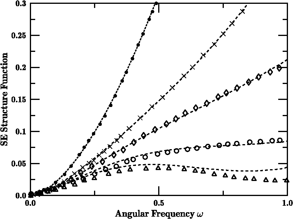 A key element of these results is the range of Rytov variance where similar results were obtained using RA versus the alternative approaches of Refs. 21 and 26. While Figs. 9 and 11 involved stretching, a single adjustment appeared to correct all cases, while no adjustment was used in Fig. 10 where the two strongest turbulence cases corresponded to values of 12.7 and 22.8. This ability of the RA to perform at high levels is consistent with the Sec. 2.3 analysis. Lastly, four prior SE MTF models, (1) (Fried’s far-field case), (2) (Fried’s near-field case), (3) Holst’s15 method where either Fried’s near-field or far-field approximation was chosen based on best fit, and (4) the method of Ref. 24, were compared with the new analytic SE MTF model (5). An RMS metric was used to compare each estimate against database-derived MTF values, weighted by frequency . The RMS results computed were , , , , and . The prequel model (4) outperformed methods (1) through (3), but the new model offered dramatic improvement (by a factor of 29) over the prequel, and greater than 100 better than the far-field approach. 5.ConclusionsThis paper’s extended high angular frequency analysis, using the methodology described in Sec. 2, has lead to a new analytic expression for the atmospheric SE MTF. This model’s RMS error of 0.000218 versus numerically integrated results represents factors of 29 improvement over the prequel,24 49 over Holst,15 and 64 over Fried’s near-field case.20 The new model exhibits diffraction-limited behavior at all angular frequencies. The primary focus of this effort was to provide systems performance engineers with an easily computed SE MTF that accounted for a thorough range of system and observational scenario conditions. Specifically, it improves evaluation of SE MTF degradation at high frequencies. This will aid trade studies in evaluating image reconstruction technique effectiveness where high frequency edge information losses are of critical concern. Augmenting the present model, a previous study37 showed that the new model, based on structure functions, can treat path-varying turbulence effects, including slant-path and valley geometries. A planned future paper will expand on these results, considering the annular aperture case (Newtonian telescopes, etc.), where the circular aperture results represent the zero central obscuration limit of the more general solution. The main caveats of the model regard the Kolmogorov spectrum used and the validity of the RA method. Regards the spectrum, we impose the requirement that , ensuring occurs in the inertial subrange. Regarding the RA method, conditions derived based on Dashen’s 30 analysis [Eqs. (31) and (35)] suggest a relatively wide range of applicability. This suitability was further tested through intercomparison with path-integral21 and Markov26 techniques. Results of the current study might also be used in an improved inverse filtering procedure [e.g., Ref. 5], though such a study is beyond the scope of the present work. In such a study, multiple range effects could be simulated, but special handling would be required to subsegment the images to apply different MTF’s in different portions of the image field. ReferencesD. Sadotet al.,
“Restoration of thermal images distorted by atmophere, using predicted atmospheric modulation transfer function,”
Infrared Phys Technol., 36
(2), 565
–576
(1995). http://dx.doi.org/10.1016/1350-4495(94)00045-M IPTEEY 1350-4495 Google Scholar
D. H. FrakesJ. W. MonacoM. J. T. Smith,
“Suppression of atmospheric turbulence in video using an adaptive control grid interpolation approach,”
in Proc. IEEE Int’l Conf. on Acoustics, Speech, and Sig. Proc.,
1881
–1884
(2001). Google Scholar
M. A. VorontsovG. W. Carhart,
“Anisoplanatic imaging through turbulent media: image recovery by local information fusion from a set of short-exposure images,”
J. Opt. Soc. Am. A, 18
(6), 1312
–1324
(2001). http://dx.doi.org/10.1364/JOSAA.18.001312 JOAOD6 0740-3232 Google Scholar
D. D. BaumgartnerB. J. Schachter,
“Improving FLIR ATR performance in a turbulent atmosphere with a moving platform,”
Proc. SPIE, 8391 839103
(2012). http://dx.doi.org/10.1117/12.917197 PSISDG 0277-786X Google Scholar
J. GillesS. Osher,
“Fried deconvolution,”
Proc. SPIE, 8355 83550G
(2012). http://dx.doi.org/10.1117/12.917234 PSISDG 0277-786X Google Scholar
J. Gilles,
“Mao-Gilles algorithm for turbulence stabilization,”
Img. Proc. On Line, 2013 173
–182
(2013). http://dx.doi.org/10.5201/ipol.2013.46 Google Scholar
J. Liuet al.,
“An efficient variational method for image restoration,”
Abstr. Appl. Anal., 2013 213536
(2013). http://dx.doi.org/10.1155/2013/213536 Google Scholar
Y. Louet al.,
“Video stabilization of atmospheric turbulence distortion,”
Inverse Probl Imag., 7 839
–861
(2013). http://dx.doi.org/10.3934/ipi 1930-8337 Google Scholar
D. Tofsted,
“Turbulence simulation: on phase and deflector screen generation,”
(2001). Google Scholar
G. PotvinJ. L. ForandD. Dion,
“Some space-time statistics of the turbulent point-spread function,”
J. Opt. Soc. Am. A, 24
(3), 753
–763
(2007). http://dx.doi.org/10.1364/JOSAA.24.002932 JOAOD6 0740-3232 Google Scholar
E. RepasiR. Weiss,
“Analysis of image distortions by atmospheric turbulence and computer simulation of turbulence effects,”
Proc. SPIE, 6941 89410S
(2008). http://dx.doi.org/10.1117/12.775600 PSISDG 0277-786X Google Scholar
A. L. RobinsonJ. SmithA. Sanders,
“An efficient turbulence simulation algorithm,”
Proc. SPIE, 8355 83550K
(2012). http://dx.doi.org/10.1117/12.919541 PSISDG 0277-786X Google Scholar
N. S. Kopeika, A System Engineering Approach to Imaging, SPIE Press, Bellingham, Washington
(1998). Google Scholar
K. Krapelset al.,
“Atmospheric turbulence modulation transfer function for infrared target acquisition modeling,”
Opt. Eng., 40
(9), 1906
–1913
(2001). http://dx.doi.org/10.1117/1.1390299 OPEGAR 0091-3286 Google Scholar
Electro-Optical Imaging System Performance, 3rd ed.SPIE Press, Bellingham, Washington
(2002). Google Scholar
J. W. Goodman, Statistical Optics, J. Wiley & Sons, New York
(1985). Google Scholar
M. C. RoggemannB. Welsh, Imaging Through Turbulence, CRC Press, Boca Raton, FL
(1996). Google Scholar
D. L. Fried,
“Statistics of a geometric representation of wavefront distortion,”
J. Opt. Soc. Am., 55
(11), 1427
–1435
(1965). http://dx.doi.org/10.1364/JOSA.55.001427 JOSAAH 0030-3941 Google Scholar
D. L. Fried,
“Untitled errata for Ref. [18],”
J. Opt. Soc. Am., 56
(3), 410E
(1966). JOSAAH 0030-3941 Google Scholar
D. L. Fried,
“Optical resolution through a randomly inhomogeneous medium for very long and very short exposures,”
J. Opt. Soc. Am., 56
(10), 1372
–1379
(1966). http://dx.doi.org/10.1364/JOSA.56.001372 JOSAAH 0030-3941 Google Scholar
M. I. Charnotskii,
“Anisoplanatic short-exposure imaging in turbulence,”
J. Opt. Soc. Am. A, 10
(3), 492
–501
(1993). http://dx.doi.org/10.1364/JOSAA.10.000492 JOAOD6 0740-3232 Google Scholar
A. McDonaldS. C. Cain,
“Parameterized blind deconvolution of laser radar imagery using an anisoplanatic optical transfer function,”
Opt. Eng., 45
(11), 116001
(2006). http://dx.doi.org/10.1117/1.2393021 OPEGAR 0091-3286 Google Scholar
J. R. DunphyJ. R. Kerr,
“Turbulence effects on target illumination by laser sources: phenomenological analysis and experimental results,”
Appl. Opt., 16
(5), 1345
–1358
(1977). http://dx.doi.org/10.1364/AO.16.001345 APOPAI 0003-6935 Google Scholar
D. Tofsted,
“Reanalysis of turbulence effects on short-exposure passive imaging,”
Opt. Eng., 50
(1), 016001
(2011). http://dx.doi.org/10.1117/1.3532999 OPEGAR 0091-3286 Google Scholar
M. I. Charnotskii,
“Statistics of the point spread function for imaging through turbulence,”
Proc. SPIE, 8014 80140W
(2011). http://dx.doi.org/10.1117/12.884248 PSISDG 0277-786X Google Scholar
M. I. Charnotskii,
“Statistical modeling of the point spread function for imaging through turbulence,”
Opt. Eng., 51
(10), 101706
(2012). http://dx.doi.org/10.1117/1.OE.51.10.101706 OPEGAR 0091-3286 Google Scholar
M. I. Charnotskii,
“Twelve mortal sins of the turbulence propagation science,”
Proc. SPIE, 8162 816205
(2011). http://dx.doi.org/10.1117/12.894550 PSISDG 0277-786X Google Scholar
M. I. Charnotskii,
“Common omissions and misconceptions of wave propagation in turbulence: discussion,”
J. Opt. Soc. Am. A, 29
(5), 711
–721
(2012). http://dx.doi.org/10.1364/JOSAA.29.000711 JOAOD6 0740-3232 Google Scholar
V. I. Tatarski, Wave Propagation in a Turbulent Medium, McGraw-Hill, New York
(1961). Google Scholar
D. H. Dashen,
“Path integrals for waves in random media,”
J. Math. Phys., 20
(5), 139
–155
(1979). http://dx.doi.org/10.1063/1.524138 JMAPAQ 0022-2488 Google Scholar
R. S. LawrenceJ. W. Strohbehn,
“A survey of clear-air propagation effects relevant to optical communications,”
Proc. IEEE, 58
(10), 1523
–1545
(1970). http://dx.doi.org/10.1109/PROC.1970.7977 IEEPAD 0018-9219 Google Scholar
M. I. Charnotskii,
“Energy conservation: a third constraint on the turbulent point spread function,”
Opt. Eng., 52
(4), 046001
(2013). http://dx.doi.org/10.1117/1.OE.52.4.046001 OPEGAR 0091-3286 Google Scholar
D. Tofstedet al.,
“Characterization of atmospheric turbulence during the NATO RTG-40 land field trials,”
Proc. SPIE, 6551 65510J
(2007). http://dx.doi.org/10.1117/12.720696 PSISDG 0277-786X Google Scholar
J. C. Kaimalet al.,
“Spectral characteristics of surface-layer turbulence,”
Q. J. Roy. Met. Soc., 98
(417), 563
–589
(1972). http://dx.doi.org/10.1002/(ISSN)1477-870X QJRMAM 0035-9009 Google Scholar
W. Presset al., Numerical Recipes in C, Cambridge University Press, Cambridge, UK
(1992). Google Scholar
M. VorontsovV. Sivokon,
“Stochastic parallel gradient descent technique for high-resolution wave-front phase-distortion correction,”
J. Opt. Soc. Am. A, 15
(10), 2745
–2758
(1998). http://dx.doi.org/10.1364/JOSAA.15.002745 JOAOD6 0740-3232 Google Scholar
D. Tofsted,
“Short-exposure passive imaging through path-varying convective boundary layer turbulence,”
Proc. SPIE, 8355 83550J
(2012). http://dx.doi.org/10.1117/12.920840 PSISDG 0277-786X Google Scholar
BiographyDavid H. Tofsted is a physicist with the U.S. Army Research Laboratory at White Sands Missile Range, New Mexico, with over 33 years in service. He received his BS degree in physics from Pennsylvania State University, Pennsylvania, in 1979, and MS and PhD degrees in electrical engineering from New Mexico State University, New Mexico, in 1992 and 2013. His research has focused on optical propagation problems, including numerical simulations of optical turbulence in the atmospheric boundary layer and its impacts on optical imaging systems. He has authored over 60 publications. |