Regularization approach to scene-based nonuniformity correction

Jun-Hyung Kim; Jieun Kim; Sohyun Kim; Joohyoung Lee; Boohwan Lee

doi:10.1117/1.OE.53.5.053105

7 May 2014 Regularization approach to scene-based nonuniformity correction

Jun-Hyung Kim, Jieun Kim, Sohyun Kim, Joohyoung Lee, Boohwan Lee

Author Affiliations +

Optical Engineering, Vol. 53, Issue 5, 053105 (May 2014). https://doi.org/10.1117/1.OE.53.5.053105

Abstract

Various scene-based nonuniformity correction (SBNUC) methods have been proposed to diminish the residual nonuniformity (RNU) of the infrared focal plane array (IRFPA) sensors. Most existing SBNUC techniques require a relatively large number of image frames to reduce the RNU. In some applications, however, there is not enough time for capturing a large number of image frames prior to the camera operation, or only several image frames are available to users. A new scene-based approach that can correct the RNU using only several image frames is proposed. The proposed method formulates the SBNUC process as an energy minimization problem. In the proposed energy function, we introduce regularization terms for the parameter regarding the responsivity of the IRFPA as well as for the true scene irradiance. Correction results are obtained by minimizing the energy function using a numerical technique. Experimental results demonstrate the effectiveness of the proposed method.

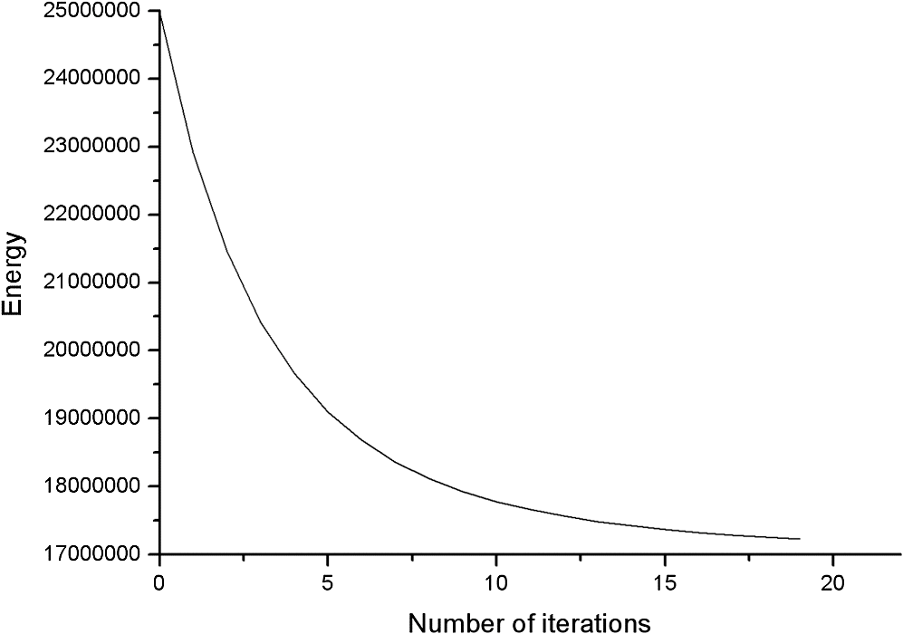
1. Introduction

The spatial noise caused by nonuniformity of individual detector elements in the infrared focal plane array (IRFPA) can limit the overall performance of imaging systems. In general, the responsivity of individual detector elements is assumed to be linear. Therefore, it is possible to correct the nonuniformity using the well-known two-point correction (TPC) method, where two blackbodies at different temperatures are employed.¹ Since the nonuniformity normally drifts in time² and the correction capability of the TPC is degraded with repeated operations,³ we need to recalibrate the IRFPA. In practice, there are two difficulties in using the TPC method to compensate the residual nonuniformity (RNU) resulting from the temporal drifit or repeated operations: (1) we have to maintain two distinct heat sources in imaging systems; and (2) real-time video operation is interrupted during the correction process.⁴

Various scene-based nonuniformity correction (SBNUC) algorithms have been proposed to solve these problems. In general, SBNUC schemes can be broadly divided into two categories: constant statistics (CS) methods⁴^–⁶ and least mean square (LMS) methods.⁷^–¹⁰ The original CS method assumes that the temporal mean and standard deviation of each pixel are constant over time and space.⁵ The performance of the original CS method is reliable as long as the assumption is valid. As pointed out in Refs. 4 and 6, however, thousands of image frames are required to hold the assumption. Zhang and Zhao⁴ proposed a local constant statistics (LCS) method, which assumes that the temporal statistics are constant in a local region around each pixel. The LCS method improved the correction performance for the same number of input frames.⁴ Later, Zuo et al.⁶ generalized the LCS method by introducing a new constraint called multiscale CS.

In the LMS methods, the correction parameters are learned by minimizing the LMS error between corrected images and desired output images. The minimization is performed frame-by-frame using the stochastic gradient descent (SGD) technique.¹¹ Since the desired output images are not available, spatially low-pass filtered input images are used as the desired ones.⁷ However, the performance of the LMS method is degraded at strong edge points as reported in Refs. 8 to 10. Thus, several methods improve the estimation accuracy of correction parameters by suppressing the influence of strong edge points in the minimization process. Vera and Torres⁸ adaptively adjust the learning rate which is a fixed parameter in the original SGD techinque, according to the local spatial standard deviations of input images. In this way, the influence of strong edge regions, where the local standard deviation is large, is reduced in the minimization process. This method is further improved in Ref. 9 to remove burn-in artifacts caused by temporally slowly-varying image regions. An approach proposed in Ref. 10 updates correction parameters only when sufficient change occurs between consecutive images.

Lately, different error functions are proposed as alternatives to the LMS error in the original LMS method.¹²^–¹⁴ Interframe registration-based LMS method¹²^,¹³ first registers the previous corrected image with the current input image by assuming that only slight translational motion exists. Then, this technique minimizes the LMS error between the previously shifted image and the currently corrected image. Vera et al.¹⁴ minimize the total variation of corrected images to obtain the correction parameters.

Although these previous SBNUC algorithms may reduce the RNU, they have a common problem: a relatively large number of image frames are required to acquire the correction parameters.¹⁵ Two recently proposed SBNUC algorithms perform NUC using several image frames¹⁶ or even only two image frames.¹⁵ These methods can achieve good performance when the relative motion in successive image frames is a small translation along vertical or horizontal directions. However, large displacements between consecutive image frames can occur in some applications.¹⁷^,¹⁸ To deal with the motion constraint of the previous approaches,¹⁵^,¹⁶ we propose a new SBNUC method that estimates the correction parameters using several image frames. In the proposed method, we utilize the prior information on the parameters regarding the responsivity and the true scene irradiance. There is no restriction on the motion in successive image frames unless it is static.

The rest of this article is organized as follows. In Sec. 2, the proposed SBNUC method is detailed. In Sec. 3, the performance of the proposed method is evaluated. Conclusion is drawn in Sec. 4.

2. Proposed Method

In this section, we first formulate an optimization problem for correcting the RNU followed by its numerical solution.

2.1.

Formulation

Let us assume that the characteristic of each detector element in the IRFPA is linear.⁵^,⁷ Then, the acquired signal $y (i, j, t)$ for the $(i, j)$ ’th detector element at time $t$ is given by

Eq. (1)

y (i, j, t) = x (i, j, t) + o (i, j, t),

where

o (i, j, t)

represents the offset of each detector element and

x (i, j, t)

indicates the scene irradiance. Here, we assume that there is no gain nonuniformity since the offset component is the dominant source of the RNU.¹⁵^,¹⁹^,²⁰ Given the image observation model [Eq. (1)], our objective is to estimate

x (i, j, t)

and

o (i, j, t)

. This problem can be solved by minimizing the proposed energy function, which consists of three terms:

Eq. (2)

E (x, o) = \sum_{t \in Ω} \sum_{i, j \in I} D (x, o) + λ_{o} C_{1} (o) + λ_{x} C_{2} (x),

where

Ω

and

I

denote the set of given image frames and the image domain, respectively.

λ_{o}

and

λ_{x}

are regularization parameters for

C_{1} (o)

and

C_{2} (x)

, respectively. The data-fidelity term

D

which measures the mismatch between the observed image and the estimates is given by

Eq. (3)

D (x, b) = {[y (i, j, t) - x (i, j, t) - o (i, j, t)]}^{2} .

Solving Eq. (3) alone is an underconstrained problem in which the number of unknowns is greater than that of equations. Thus, a regularization approach is taken to estimate $x (i, j, t)$ and $o (i, j, t)$ in this work. The regularization term for the offset $o (i, j, t)$ is defined as follows:

Eq. (4)

C_{1} (o) = {[\frac{\partial o (i, j, t)}{\partial t}]}^{2} .

$C_{1} (o)$ is derived from the observation that the offset changes very slowly in time.⁷^,⁹ In other words, the offset remains almost constant for several consecutive image frames.²⁰ This regularization term favors the offset with small changes along the time axis. If we correctly estimate $o (i, j, t)$ for the given image frames, their temporal variation is negligible, which means that $C_{1} (o)$ is very close to zero.

The last term $C_{2} (x)$ in Eq. (2) is introduced to regularize the scene irradiance $x (i, j, t)$ . In general, $x (i, j, t)$ is smooth in the spatial domain. This fact is implictly used in the original LMS method, where the desired image is the spatially low-pass filtered input image.⁷ Thus, it is natural for us to require $x (i, j, t)$ to be smooth in the spatial domain. Since the degree of the spatial smoothness can be measured via the image gradient, $C_{2} (x)$ is given by

Eq. (5)

C_{2} (x) = w_{i} [y (i, j, t)] {[\frac{\partial x (i, j, t)}{\partial i}]}^{2} + w_{j} [y (i, j, t)] {[\frac{\partial x (i, j, t)}{\partial j}]}^{2} .

The smoothness term $C_{2} (x)$ is proportional to the magnitude of the spatial intensity change of the scene irradiance. Therefore, the smoother the scene irradiance is, the smaller the value of $C_{2} (x)$ is. However, the smoothness constraint is not appropriate at edge points as pointed out in Sec. 1. Since the spatial variation of $x (i, j, t)$ is normally greater than that of RNU,² the large spatial variation in the input image $y (i, j, t)$ is mainly due to the edge points of $x (i, j, t)$ . We adaptively adjust the effect of the smoothness constraint according to the gradient of $y (i, j, t)$ . The weighting factors $w_{i} [y (i, j, t)]$ and $w_{j} [y (i, j, t)]$ in Eq. (5) are defined as follows

Eq. (6)

w_{i} (y) = {[{| \frac{\partial y (i, j, t)}{\partial i} |}^{γ} + ε]}^{- 1},

Eq. (7)

w_{j} (y) = {[{| \frac{\partial y (i, j, t)}{\partial j} |}^{γ} + ε]}^{- 1} .

The exponent $γ$ controls the sensitivity to the spatial gradients of $y (i, j, t)$ and $ε$ is a small constant that prevents dividing by zero. Since the weighting factors are inversely proportional to the spatial gradients of $y (i, j, t)$ , the smoothness constraint has little effect on edge regions. These weighting factors are the same as smoothness weights for the image smoothing operator in Ref. 21.

2.2.

Numerical Solution

The proposed energy function $E (x, o)$ in Eq. (2), a function of two variables, is nonconvex. We minimize the energy function by solving two convex subproblems in an alternating way with initial estimates $x^{(0)} = y$ and $o^{(0)} = 0$ :

Eq. (8)

x^{(n)} = \underset{x}{argmin} E [x, o^{(n - 1)}],

Eq. (9)

o^{(n)} = \underset{o}{argmin} E [x^{(n)}, o] .

The above process is repeated until there is no significant change in the estimates $x^{(n)}$ and $o^{(n)}$ .

We compute the partial derivative of Eq. (2) with respect to $x$ in order to solve Eq. (8). First, we represent Eq. (2) in matrix notation as follows:

Eq. (10)

\sum_{t \in Ω} {[y (t) - x (t) - o (t)]}^{T} [y (t) - x (t) - o (t)] + λ_{x} [x {(t)}^{T} D_{i}^{T} W_{i} (t) D_{i} x (t) + x {(t)}^{T} D_{j}^{T} W_{j} (t) D_{j} x (t)],

where

y (t)

,

x (t)

, and

o (t)

are the lexicographically ordered vectors corresponding to the acquired signal, the scene irradiance, and the offset at time

t

, respectively.

W_{i} (t)

and

W_{j} (t)

denote diagonal matrices containing values of the weighting factors

w_{i} (y)

and

w_{j} (y)

at time

t

, respectively.

D_{i}

and

D_{j}

are the backward difference operators along

i

and

j

directions, which approximate the spatial partial gradients. Note that the regularization term for the offset

C_{1} (o)

is omitted in Eq. (10) since

C_{1} (o)

is constant with respect to

x

. Then,

\partial E / \partial x

in matrix notation is given by

Eq. (11)

\frac{\partial E}{\partial x} = \sum_{t \in Ω} [A (t) x (t) - b (t)],

where

Eq. (12)

A (t) = λ_{x} [D_{i}^{T} W_{i} (t) D_{i} + D_{j}^{T} W_{j} (t) D_{j}],

Eq. (13)

b (t) = y (t) - o (t) .

Therefore, we solve a large system of linear equations [i.e., $A (t) x (t) = b (t)$ ] for each $x (t)$ . The conjugate-gradient (CG) method is used to solve the linear equations in this work since the matrix $A$ is sparse, symmetric, and positive definite.²²

We rewrite Eq. (2) in different matrix notation from that represented in Eq. (10) to solve Eq. (9):

Eq. (14)

\sum_{i, j \in I} {[y (i, j) - x (i, j) - o (i, j)]}^{T} [y (i, j) - x (i, j) - o (i, j)] + λ_{o} [o {(i, j)}^{T} D_{t}^{T} D_{t} o (i, j)],

where

y (i, j)

,

x (i, j)

, and

o (i, j)

are vectors formed by lexicographically stacking the acquired signal, the scene irradiance, and the offset in the time domain, respectively, for each detector element located in

(i, j)

.

D_{t}

is the temporal backward difference operator. Similar to Eq. (10), we exclude the regularization term

C_{2} (x)

in Eq. (14) since it is constant with respect to

o

. Differentiation with respect to

o

produces

Eq. (15)

\frac{\partial E}{\partial o} = \sum_{i, j \in I} [A^{'} o (i, j) - b^{'} (i, j)],

where

Eq. (16)

A^{'} = I + λ_{o} D_{t}^{T} D_{t},

Eq. (17)

b^{'} (i, j) = y (i, j) - x (i, j) .

$I$ denotes identity matrix in Eq. (16). The CG method is used here again to obtain the values of the offset for each $o (i, j)$ .

3. Simulation Results

To our best knowledge, no study has been reported on correcting the RNU with several image frames that have large displacements. Therefore, no comparison is made with existing SBNUC methods in this work. The regularization parameters are empirically set to $λ_{o} = 6$ , $λ_{x} = 0.1$ for all experiments in this article, and the value of $γ$ is determined to be 0.2. At first, we test the convergence of the proposed method with eight synthetic images as shown in Fig. 1. The eight images are generated by adding the artificial offset⁹^,¹⁵ to calibrated infrared images caputured by a $320 \times 256$ InSb focal plane array camera operating in the 3 to 5 μm range. The RNU is generally composed of two patterns, the low-frequency one and white noise-like one as reported in Ref. 23. However, only the white noise-like pattern is usually prominent to observers together with natural scenes. This is due to the masking effect of the human visual system, which attenuates contrast sensitivity at low-spatial frequencies.²⁴ Therefore, the artificial offset is generated as realizations of independent identically distributed Gaussian random variables.⁹

Fig. 1

Simulated nonuniformity images.

We plot the proposed energy function in Eq. (2) against the number of iterations. As shown in Fig. 2, the value of the energy function drops quickly. We obtain good results with 11 iterations in our expeirments. In Fig. 3, we present images corrected by the proposed NUC method. Close-up views of some parts of the images are depicted in Fig. 3(b) to help the reader observe the visual quality improvement. The proposed method produces acceptable results no matter how complex the spatial distribution is, as shown in Fig. 3.

Fig. 2

Convergence of the proposed method.

Fig. 3

Nonuniformity correction (NUC) results on the synthetic images. (a) Whole images. (b) Close-ups of the input (left) and the proposed (right).

We investigate the effect of the number of input images on the estimated scene irradiance using the eight synthetic images. Table 1 shows the peak signal-to-noise ratio results for different numbers of input images. As the number of input images increases, we can obtain more accurate results. This can be described by the fact that the information gained from consecutive image frames leads to high-quality NUC results and enhanced temporal consistency in the offset. Note that, however, raising the number of input images increases processing time. Thus, selecting a proper number of input images demands trade-off between the computational complexity and the image quality.

Table 1

Peak signal-to-noise ratio results of the proposed method with various numbers of input images.

Image #	Input	2 images	4 images	6 images	8 images
1	27.65	29.61	31.4	32.19	32.6
2	27.64	29.52	31.37	32.17	32.6
3	27.62	—	31.34	32.19	32.65
4	27.59	—	31.27	32.17	32.64
5	27.59	—	—	32.12	32.62
6	27.57	—	—	32.01	32.55
7	27.54	—	—	—	32.48
8	27.52	—	—	—	32.38
Average	27.59	29.57	31.35	32.14	32.57

We also perform an experiment on two sets of real infrared images as shown in Fig. 4. We have collected the two sets of images using a $640 \times 512$ InSb focal plane array camera operating in the 3 to 5 μm range. One set of images in Fig. 4(a) shows drastic intensity changes among them due to atmospheric effects. The other set of images in Fig. 4(b) has relatively large motion. Objective results for the proposed method are provided in Table 2. We employ a roughness metric⁸^,⁹^,¹⁵ which is defined by

Eq. (18)

ρ = \frac{{‖ h_{1} * I ‖}_{1} + {‖ h_{2} * I ‖}_{1}}{{‖ I ‖}_{1}},

where

h_{1}

and

h_{2}

are horizontal and vertical difference filters, respectively,

I

represents the image under test,

{‖ ‖}_{1}

is the

L_{1}

norm, and * denotes discrete convolution. The roughness metric

ρ

measures the amount of high-frequency energy due to the RNU. As pointed out in Ref. 9, the metric cannot distinguish between true high-frequency energy and that from the RNU. However, the metric can be a useful indicator of the RNU to some degree when taken along with subjective evaluation.⁹ The correction results of the proposed method are depicted in Figs. 5 and 6. Similar to the simulated nonuniformity case, our method consistently suppresses the RNU as shown in Figs. 5(b) and 6(b). We also present the difference images between the input and the corrected in Fig. 7 to visualize the RNU corrected by the proposed method.

Fig. 4

Real infrared images.

Table 2

Roughness results for real images.

Image #	Fig. 4(a)		Fig. 4(b)
Image #	Input	Proposed	Input	Proposed
1	0.2211	0.0717	0.2183	0.0626
2	0.1290	0.0798	0.3981	0.0618
3	0.4618	0.0648	0.4338	0.0465
4	0.7389	0.0484	—	—
5	0.3975	0.0685	—	—

Fig. 5

NUC results on images shown in Fig. 4(a). (a) Whole images. (b) Close-ups of the input (top) and the corrected (bottom).

Fig. 6

NUC results on images shown in Fig. 4(b). (a) Whole images. (b) Close-ups of the input (top) and the corrected (bottom).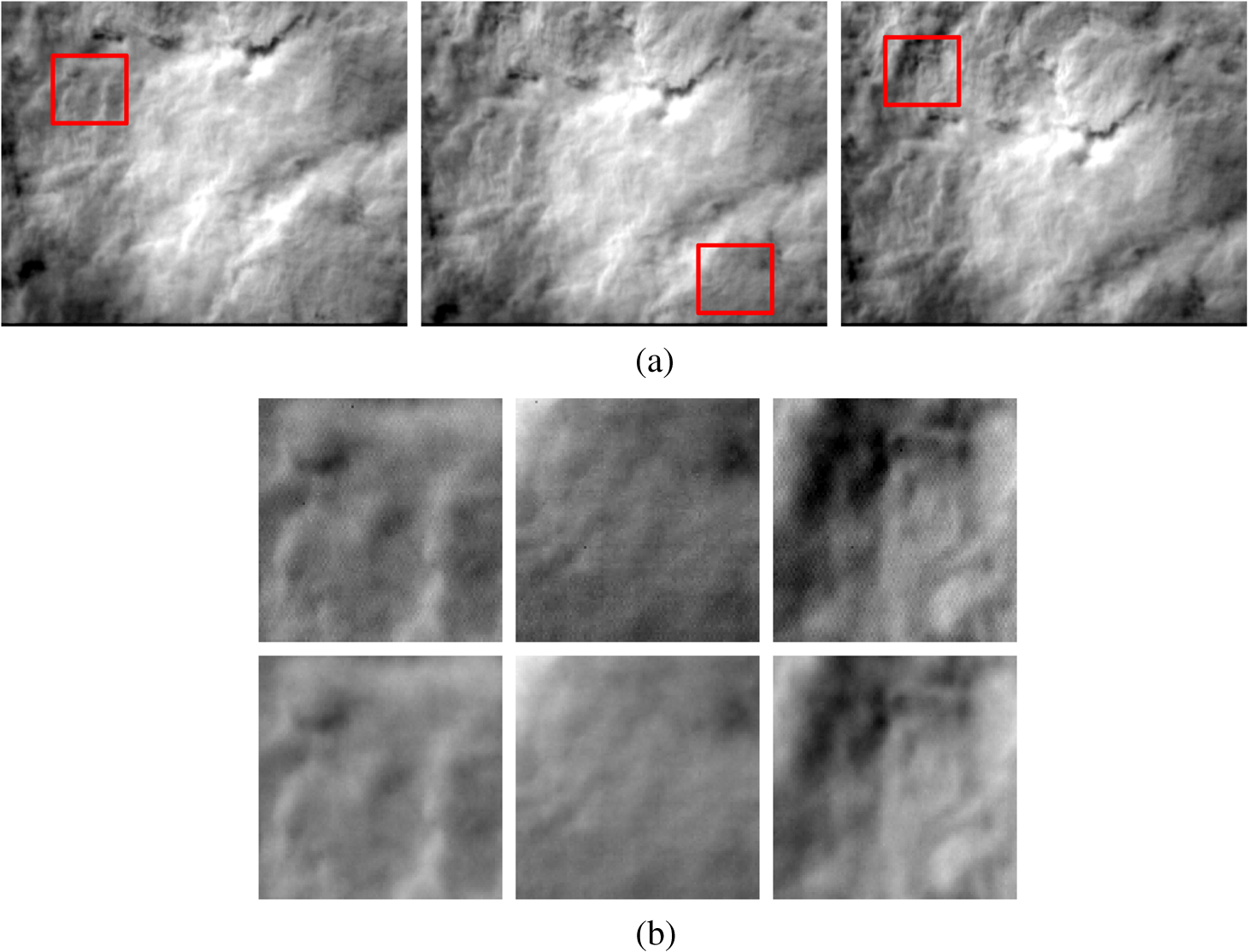

Fig. 7

Difference images between the input and the corrected for (a) the fifth image in Fig. 4(a) and the third image in Fig. 4(b).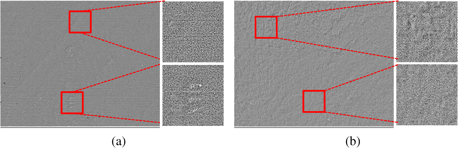

We have implemented the proposed method using C language. The simulation is performed on a PC with an Intel i7 3.40-GHz CPU and 4-GB memory. Our optimization procedure takes 5.6 and 3.8 s for the set of images in Figs. 4(a) and 4(b), respectively.

4. Conclusion

We presented a regularization approach to SBNUC with several image frames. Our work formulated the SBNUC process as the energy minization problem that incorporates the slowly varying nature of the detector responsivity and the smoothness constraint for the scene irradiance. In the proposed method, no assumption was made about the motion among input images except that the motion is static. Therefore, the proposed method can be used in applications where only several image frames are available and large displacements exist among the given images. Simulation results on both synthetic and real infrared images demonstrated that the proposed method can reduce the RNU. In future works, we plan to apply more advanced numerical techniques to reduce the computational complexity of the proposed method.

References

1.

D. L. PerryE. L. Dereniak, “Linear theory of nonuniformity correction in infrared staring sensors,” Opt. Eng., 32 (8), 1854 –1859 (1993). http://dx.doi.org/10.1117/12.145601 OPEGAR 0091-3286 Google Scholar

2.

W. GrossT. HierlM. Schulz, “Correctability and long-term stability of infrared focal plane arrays,” Opt. Eng., 38 (5), 862 –869 (1999). http://dx.doi.org/10.1117/1.602055 OPEGAR 0091-3286 Google Scholar

3.

L. Shkedyet al., “Megapixel digital InSb detector for midwave infrared imaging,” Opt. Eng., 50 (6), 061008 (2011). http://dx.doi.org/10.1117/1.3572163 OPEGAR 0091-3286 Google Scholar

4.

C. ZhangW. Zhao, “Scene-based nonuniformity correction using local constant statistics,” JOSA A, 25 (6), 1444 –1453 (2008). http://dx.doi.org/10.1364/JOSAA.25.001444 JOAOD6 1084-7529 Google Scholar

5.

J. G. HarrisY.-M. Chiang, “Nonuniformity correction of infrared image sequences using the constant-statistics constraint,” IEEE Trans. Image Process., 8 (8), 1148 –1151 (1999). http://dx.doi.org/10.1109/83.777098 IIPRE4 1057-7149 Google Scholar

6.

C. Zuoet al., “Scene-based nonuniformity correction method using multiscale constant statistics,” Opt. Eng., 50 (8), 087006 (2011). http://dx.doi.org/10.1117/1.3610978 OPEGAR 0091-3286 Google Scholar

7.

D. A. Scribneret al., “Adaptive nonuniformity correction for ir focal-plane arrays using neural networks,” Proc. SPIE, 1541 100 –109 (1991). http://dx.doi.org/10.1117/12.49324 PSISDG 0277-786X Google Scholar

8.

E. VeraS. Torres, “Fast adaptive nonuniformity correction for infrared focal-plane array detectors,” EURASIP J. Appl. Signal Process., 2005 1994 –2004 (2005). http://dx.doi.org/10.1155/ASP.2005.1994 1110-8657 Google Scholar

9.

R. C. Hardieet al., “Scene-based nonuniformity correction with reduced ghosting using a gated lms algorithm,” Opt. Express, 17 (17), 14918 –14933 (2009). http://dx.doi.org/10.1364/OE.17.014918 OPEXFF 1094-4087 Google Scholar

10.

A. RossiM. DianiG. Corsini, “Temporal statistics de-ghosting for adaptive non-uniformity correction in infrared focal plane arrays,” Electron. Lett., 46 (5), 348 –349 (2010). http://dx.doi.org/10.1049/el.2010.3559 ELLEAK 0013-5194 Google Scholar

11.

L. Bottou, “Large-scale machine learning with stochastic gradient descent,” in Proc. COMPSTAT’2010, 177 –186 (2010). Google Scholar

12.

C. Zuoet al., “Scene-based nonuniformity correction algorithm based on interframe registration,” JOSA A, 28 (6), 1164 –1176 (2011). http://dx.doi.org/10.1364/JOSAA.28.001164 JOAOD6 1084-7529 Google Scholar

13.

C. Zuoet al., “Improved interframe registration based nonuniformity correction for focal plane arrays,” Infrared Phys. Technol., 55 (4), 263 –269 (2012). http://dx.doi.org/10.1016/j.infrared.2012.04.002 IPTEEY 1350-4495 Google Scholar

14.

E. VeraP. MezaS. Torres, “Total variation approach for adaptive nonuniformity correction in focal-plane arrays,” Opt. Lett., 36 (2), 172 –174 (2011). http://dx.doi.org/10.1364/OL.36.000172 OPLEDP 0146-9592 Google Scholar

15.

C. Zuoet al., “A two-frame approach for scene-based nonuniformity correction in array sensors,” Infrared Phys. Technol., 60 190 –196 (2013). http://dx.doi.org/10.1016/j.infrared.2013.05.001 IPTEEY 1350-4495 Google Scholar

16.

C. Zuoet al., “Scene based nonuniformity correction based on block ergodicity for infrared focal plane arrays,” Optik, 123 (9), 833 –840 (2012). http://dx.doi.org/10.1016/j.ijleo.2011.06.050 OTIKAJ 0030-4026 Google Scholar

17.

M. Maoet al., “Based on airborne multi-array butting for IRFPA staring imagery,” Proc. SPIE, 7658 765858 (2010). http://dx.doi.org/10.1117/12.865976 Google Scholar

18.

C. R. del BlancoF. JaureguizarN. García, “Robust tracking in aerial imagery based on an ego-motion bayesian model,” EURASIP J. Adv. Signal Process., 2010 1 –18 (2010). http://dx.doi.org/10.1155/2010/837405 1110-8657 Google Scholar

19.

E. GurevichA. Fein, “Maintaining uniformity of ir focal plane arrays by updating offset correction coefficients,” Proc. SPIE, 4820 809 –820 (2003). http://dx.doi.org/10.1117/12.453552 Google Scholar

20.

O. Nesheret al., “Digital cooled insb detector for ir detection,” Proc. SPIE, 5074 120 –129 (2003). http://dx.doi.org/10.1117/12.498154 PSISDG 0277-786X Google Scholar

21.

Z. Farbmanet al., “Edge-preserving decompositions for multi-scale tone and detail manipulation,” ACM Trans. Graph., 27 (3), 1 –67 (2008). http://dx.doi.org/10.1145/1360612 ATGRDF 0730-0301 Google Scholar

22.

B. P. Flanneryet al., Numerical Recipes in C, Press Syndicate of the University of Cambridge, New York (1992). Google Scholar

23.

G. Gershonet al., “3 Mega-pixel InSb detector with 10 μm pitch,” Proc. SPIE, 8704 870438 (2013). http://dx.doi.org/10.1117/12.2015583 PSISDG 0277-786X Google Scholar

24.

P. J. BexS. G. SolomonS. C. Dakin, “Contrast sensitivity in natural scenes depends on edge as well as spatial frequency structure,” J. Vision, 9 (10), 11 –19 (2009). http://dx.doi.org/10.1167/9.10.1 1534-7362 Google Scholar

Biography

Jun-Hyung Kim received his BS and PhD degrees in electronic engineering from Korea University in 2006 and 2012, respectively. He has worked for the Agency for Defense Development since 2012. His current research interests are in the area of image processing and infrared imaging system. He is a member of SPIE.

Jieun Kim received her BS degree in electrical engineering from Busan National University in 2002, and her MS degree in electrical engineering from KAIST in 2004. She has worked for the Agency for Defense Development since 2004. Her current interests include digital image processing, target detection, and tracking.

Sohyun Kim is currently a research member at the Agency for Defense Development in Korea, and has over 10 years of experience in developing electro-optic systems. Her experience includes target detection algorithm design and real-time implementation for video tracker for infrared images. She holds a BS in physics from Sogang University and an MS in information and communications from Gwangju Institute of Science and Technology.

Joohyoung Lee received his BS and MS degress in electronics engineering from Dankuk University, Republic of Korea, in 1990 and 1992, respectively. Since 1992, he has been a principal researcher in the Electro-Optics Laboratory at the Agency for Defense Development. His research interests include analog and digital signal processing for IRST, low-noise electronics, IRST system test and evaluation for small target detection.

Boohwan Lee received his BS, MS, and PhD degrees in electrical engineering and computer science from Kyungpook National University, Daegu, Republic of Korea in 1991, 1993, and 2006, respectively. He has worked as a principal researcher for the Agency for Defense Development since 1993. His current interests include digital image processing, target detection, and tracking.

CC BY: © The Authors. Published by SPIE under a Creative Commons Attribution 4.0 Unported License. Distribution or reproduction of this work in whole or in part requires full attribution of the original publication, including its DOI.

Citation Download Citation

Jun-Hyung Kim, Jieun Kim, Sohyun Kim, Joohyoung Lee, and Boohwan Lee "Regularization approach to scene-based nonuniformity correction," Optical Engineering 53(5), 053105 (7 May 2014). https://doi.org/10.1117/1.OE.53.5.053105

Published: 7 May 2014

Access the abstract

JOURNAL ARTICLE
7 PAGES

DOWNLOAD PAPER SAVE TO MY LIBRARY

GET CITATION

CITATIONS

Cited by 2 scholarly publications.

Explore citations on Lens.org

KEYWORDS

Scene based nonuniformity corrections

Nonuniformity corrections

Sensors

Infrared radiation

Infrared imaging

Image filtering

Optical engineering

1.

Introduction

2.

Proposed Method

2.1.

Formulation

Eq. (1)

Eq. (2)

Eq. (3)

Eq. (4)

Eq. (5)

Eq. (6)

Eq. (7)

2.2.

Numerical Solution

Eq. (8)

Eq. (9)

Eq. (10)

Eq. (11)

Eq. (12)

Eq. (13)

Eq. (14)

Eq. (15)

Eq. (16)

Eq. (17)

3.

Simulation Results

Fig. 1

Fig. 2

Fig. 3

Table 1

Eq. (18)

Fig. 4

Table 2

Fig. 5

Fig. 6

Fig. 7

4.

Conclusion

References

Biography

Show All Keywords

Keywords/Phrases

Search In:

Publication Years