|
|
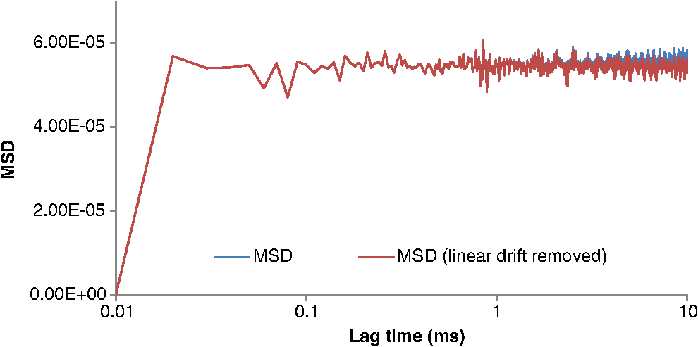
1.IntroductionOur laboratory is interested in measuring the mechanical properties of a biological object, the primary cilium.1 Optical traps provide a localized noncontact method to apply a well-controlled force while simultaneously permitting the observation of the deformation (bending) of this organelle. Here, we present our progress toward this goal by demonstrating our ability to accurately measure the spring constant of our optical trap applied to a cylindrical object, in this case an Escherichia coli bacterium. Although use of optical traps2 to apply forces to spherical and near-spherical objects is well understood in the context of Mie scattering and its generalizations,3–9 trapping cylindrical objects such as bacteria and certain virus particles has largely consisted of qualitative experiments,10–12 and use of scattering models to quantify the optical trapping of slender, cylindrical objects is greatly complicated by geometry.13–17 Use of approximate methods18 including the discrete-dipole approximation19,20 the T-matrix,21 or the finite-difference time-domain22 to calculate the applied force is one common approach, but accurate calculation of the applied force (equivalently, the trap stiffness) requires detailed trapping beam specifications; knowledge of the refractive index of both the trapped object and the solvent; viscosity of solvent; and size, shape, and composition of the trapped particle, and typically assumes that the trapped object is homogeneous. For our experimental case of interest, none of this information is readily available and may require additional complex measurements to obtain. Similarly, optical trap calibration methods involving measurements of the power spectrum23,24 or scattering efficiencies25–27 have only been experimentally verified using spherical objects. Consequently, alternative methods of calculating the applied force based on particle tracking have been developed.28–30 The primary cilium31 is a singular protruding hair-like organelle possessed by most mammalian differentiated cells, genetically related to flagella, but in contrast to motile cilia present on some specialized tissue (e.g., airway epithelia), it does not actively move. Cilia are slender, protruding cylinders, approximately 0.2 μm in diameter, ranging in length from several to tens of microns and are anchored at one end to the centrosome within the cell body. A large and still growing body of evidence has demonstrated that the primary cilium coordinates an ever-lengthening list of cell signaling pathways including Hedgehog, Wnt, platelet-derived growth factor receptor alpha, and the polycystins PC1 and PC2.32–47 The primary cilium has recently emerged as an organizing center for a wide range of cellular functions including environmental sensing of light,48 odorants49 and osmolarity,50 mechanosensation,51,52 cell development,32 migration53 and differentiation,54 and planar cell polarity.46 The mechanotransduction response has been shown to significantly modify many cellular functions and yet is currently the least-understood ciliary function due to a lack of information about the mechanical properties of the sensor. In contrast to measurements that apply a known disturbance with fluid flow,55,56 optical trapping of cilia and flagella could provide improved information about the mechanical properties of these important organelles. Specifically, it is possible to measure the bending modulus57,58 and generated force,59,60 both of which modulate the biological role of motile cilia and flagella (mucociliary transport and microorganism propulsion) and sensory cilia (flow sensing).51,52 Finally, the capability of near-simultaneous trapping and observation of a biological response (for example, intracellular ratiometric imaging)1,37 could provide improved understanding of the biological role of this organelle. In the present study, we have constructed a calibrated optical trap apparatus that provides near real-time measurements of the transverse spring constant without requiring knowledge of optical properties of the trapped object, suspending solvent, and trapping beam geometry. Because the primary cilium is anchored at one end to the cell and thus a more complicated system than a free particle, we demonstrate here a first step—measuring the trapping force applied to an E. coli bacterium, a rod-shaped bacterium 1 μm in diameter and 3 μm long. 2.Principles of Optical Tweezer OperationAs constructed,61,62 optical tweezers create a single-beam three-dimensional (3-D) potential well due to a spatial gradient of the electric field, created by focusing a laser beam with a high-numerical-aperture microscope objective. Objects possessing a refractive index greater than the surrounding fluid medium experience a spring-like restoring force as they move away from the trap center. The trapped particles thus execute a modified form of Brownian motion due to the confining potential well. For a particle undergoing free one-dimensional Brownian motion, the mean-squared displacement (MSD) relationship is given by the well-known diffusion expression63 where the is the diffusion constant for the particle, the angle brackets indicate an average over all time, and is the lag-time. A particle confined within a Gaussian potential well (corresponding to the optical trapping by a focused Gaussian beam) presents a modified MSD relationship64,65 where is the Boltzmann constant, is the temperature of the fluid medium, is the Stokes (viscous) drag coefficient of the trapped particle ( for a sphere with radius suspended in a fluid with viscosity ), and is the spring constant of the optical trap. Note that .While the spring constant and Stokes drag coefficient can be calculated analytically for the idealized case of a homogeneous spherical particle, a homogeneous suspending fluid, and aberration-free Gaussian beams, in general it is not possible to analytically calculate the spring constant of nonspherical particles of unknown composition trapped within an aberrated beam. Because our eventual goal is to calculate the force applied to a slender cylinder, we developed an algorithm based on particle tracking and fitted the calculated MSD curve using two free parameters corresponding to and . We first track the position of a trapped object with a quadrant photodiode (QPD), calculate the MSD of the particle’s trajectory, and then use a fitting algorithm in which the spring constant and viscous drag are free parameters to calculate the stiffness of the optical trap. That is, measuring the trajectory of a trapped particle allows the calculation of the gradient forces generated by the optical trap without a priori knowledge of the physical properties of the trapped object. 3.System Hardware Configuration and Software Architecture3.1.Hardware ConfigurationThe laser tweezer apparatus shown in Fig. 1 is largely the same as discussed previously61 and operates as a single-beam 3-D trap. The source was a 0.5-W diode-pumped Nd:YAG continuous-wave single-mode laser. The optical tweezer was aligned to the optical axis of the microscope (Leica DM6000B, Wetzlar, Germany) using a 5-degree-of-freedom (-axis, -axis, -axis, pitch, and yaw) mount. The laser beam was expanded to fill the back aperture of the objective lens. The objective lens used was a Leica 63X NA 0.9 U-V-I HCX long working distance plan apochromat dipping objective. The tweezer couples into the microscope through a lateral port, providing direct optical access to the fluorescence turret. A side-looking 1064-nm dichroic mirror (Chroma Technology, Bellows Falls, Vermont) mounted within the fluorescence turret provides the ability to perform the normal (visible) transillumination microscope viewing while the tweezers are operating. A KG-1 IR cutoff filter (Newport, Irvine, California) inserted above the fluorescence turret prevents the observation of the tweezer spot by a camera during operation. The trapping beam applies a force to objects by moving the microscope sample stage (Prior Proscan II Motorized H101/2 Stage); the trapping beam does not move. Fig. 1Hardware configuration of the laser tweezer, microscope, and quadrant photodiode (QPD) data acquisition system. Tweezer beam path is indicated by a solid line. Components labeled as follows: (a) Tweezer module. (b) Side-looking dichroic mirror located in fluorescence turret. (c) Objective lens. (d) Sample plane. (e) Condenser lens. (f) Dichroic mirror. (g) QPD. (h) Tube lens. (i) Camera. (j) Five-degree-of-freedom tweezer mount. (k) Transillumination stage. (l) Incubator. (m) QPD data acquisition module. (n) Computer. Inset: photograph of experimental apparatus. 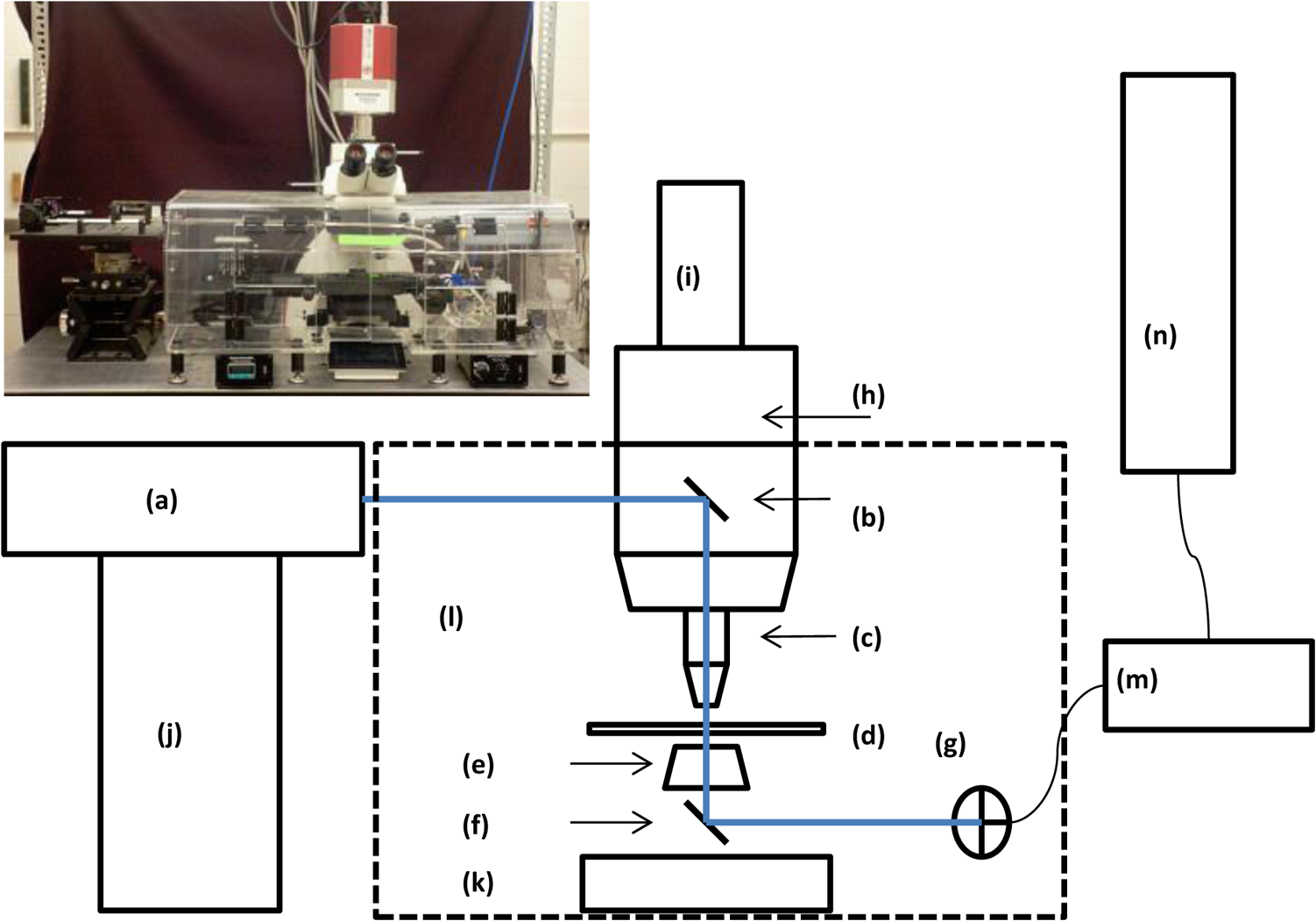 To record the movement of a trapped object, a QPD (first sensor model QP50-6-SD2) records the location of the trapping beam centroid. The QPD is located downstream from the condenser lens. Use of a dichroic mirror (Qoptic Microbench, Fairport, New York) and laser line filter (1064 nm, Edmund Optics, Barrington, New Jersey) ensures that only the Nd:YAG light is incident on the QPD. Intensities were converted to voltage readouts within the QPD housing and then transferred to a National Instruments data acquisition device. This device recorded voltages at a user-specified frequency and exported a digital record of particle positions to the host computer to be saved and analyzed later. 3.2.Software Architecture3.2.1.Tracking protocolWe created a virtual instrument (VI) environment in LabView 2010 with a front panel that allows for customization of sampling frequency and duration of data acquisition. Our tracking VI recorded voltage outputs from the QPD, normalized the data via a reference voltage to remove the circuit noise, and displayed the particle information in real time on the front panel. Figure 2 shows the flow of data through the VI, and Fig. 3 presents an example of the VI’s voltage/position readout. Fig. 2Flowchart detailing data progression within the data acquisition virtual instrument (VI). The incoming signal for the QPD is constantly pinged while the VI is running, allowing the user the ability to see a real-time feed of the laser spot on the surfaces of the QPD. 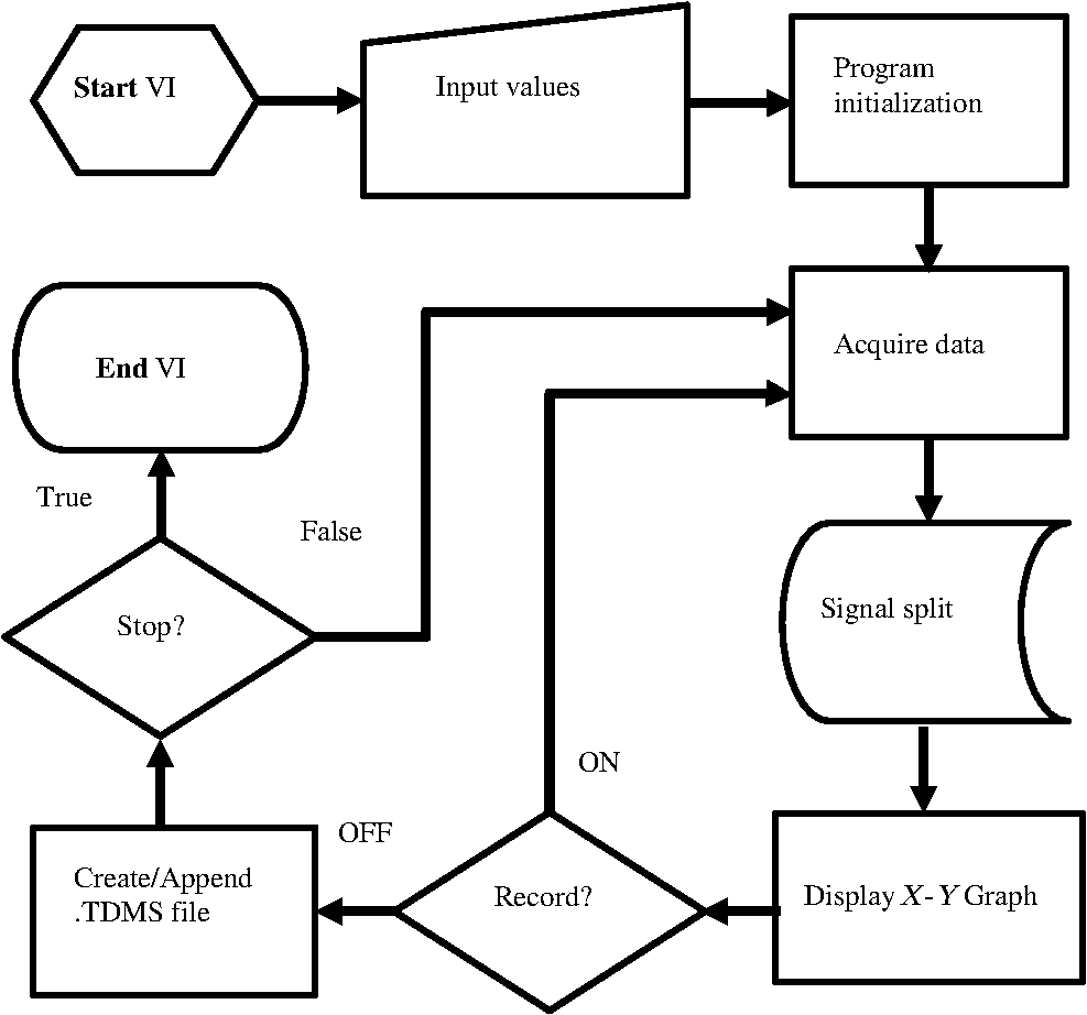 Fig. 3A sample of raw QPD output (‘X’ and ‘Y’ represent orthogonal directions). The dip is characteristic of a microsphere entering the trap.  The recorded datasets are then converted and stored as .TDMS binary files, which are used for their low data-loss rate at high sampling frequency and low memory footprint. This file can then be directly imported into our MATLAB analysis algorithm. Stock data analysis methods are not well suited for the large data files produced by high sampling rates. Therefore, an algorithm was developed to manage the large sets of acquired experimental data. All the analysis procedures are called using the function QPDanalysisBulk(TDMSFolder,TDMSfileID,f). This function has user input variables for the root directory of the .TDMS file to be analyzed and the filename of said .TDMS. 3.2.2.TDMS conversion to .MAT file typeIn order to begin the data analysis, our algorithm first converts the data from the .TDMS file into a .MAT file type for MATLAB to quickly perform the rest of the data analysis. The called function, convertTDMS(true, TDMSfileID), has been developed within a community of developers since late 2009. The function can be found via the MATLAB Central File Exchange and is offered open source to those who wish to make their own additions to the development of the code. In our toolbox, we utilized version 9 of the software and made no major changes to the function. 3.2.3.Calculate the mean-square-displacement of trajectoryWith our time-series voltage data loaded into MATLAB, the algorithm proceeds to calculate the MSD for the trajectory of the trapped particle. For any given trajectory discretized into time steps consisting of overlapping time intervals of duration , the position autocorrelation function is defined as63 The MSD(PosArray) function iteratively calculates the MSD for each lag-time, . PosArray is an array where each row is a position vector for a specific time. The function utilizes the fact that MATLAB can efficiently vectorize calculations on an entire array rather than computing them element-by-element. For example, the deltaCoords variable, which is the difference in positions between two row-vectors separated by , is computed by deltaCoords = PosArray[(1+dt:end),(1:2)]—PosArray[(1:end-dt),(1:2)]. This allows us to use the sum(deltaCoords^2, 2) function to sum each of the squares of the deltaCoord variable’s row elements and to finally take the average over all times for each . 3.2.4.Remove linear drift of MSDThe MSD curve can be split into roughly two sections. The initial (short-time) section of the curve represents an inertial timescale, whereas the latter section represents a long time limit corresponding to the restoring force of the optical trap. However, the long time limit is often not reached and as a result, the calculated MSD contains a linear drift. This experimental artifact is removed through the use of the function RemoveLinarDrift(MSDArray,maxlagtime,freq). The function first applies a linear regression to the long-time calculated MSD data. The linear regression is then subtracted from the experimentally acquired MSD data. The corrected MSD data allow the fitting of the idealized curve equation to the experimental data. An example of this curve can be seen in Fig. 4, which shows the removal of linear drift and resultant, corrected MSD. 3.2.5.Fit primary dataset to idealized relationship and store fitting parametersOnce the experimental data have been corrected with the linear drift of the long-term limit removed, the algorithm fits the data to the idealized MSD function. Since our data have an arbitrary length and time units, we must introduce two conversion constants, (normalized volts per meter) and (seconds per desired time unit). The new model can be expressed as Thus, our model can be expressed in terms of and To enhance our fitting routine’s accuracy, we first fit the long-time portion of our data with a linear model to obtain the value of . Next, we fit our data using a robust nonlinear least squares fit, supported by the MATLAB Curve Fitting toolbox. During this process, the stored value of is substituted into the model so that is the only free parameter. A graph of this fit is then exported as a MATLAB .FIG file and a high-resolution .PNG to the root folder. Figure 5 details an example of the quality of the fit achieved by the algorithm. Utilizing the relationships of the constants and , the software then solves for the spring and diffusion constants for the dataset. Finally, these values are stored in their own array to be appended with more values down the line. Fig. 5Example of the results from the curve-fitting routine for the MSD data shown in Fig. 4. Note the fitting of the long time-scale portion of the graph lies nearly along the average, allowing for an accurate reading of the fitting constants. 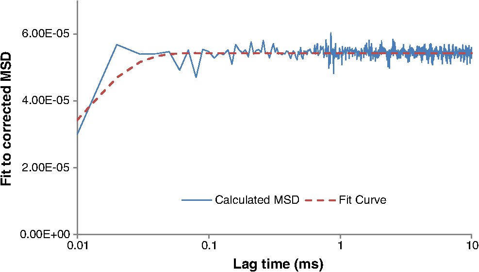 3.2.6.Subdivide primary dataset into data blocksDuring QPD data acquisition, it is sometimes observed that a second object either passes through the trapping beam or is even trapped as well, resulting in either two trapped objects or the initial object being ejected from the trap. This results in QPD data containing position jumps not characteristic to confined Brownian motion, requiring sections of the QPD data to be excised. To ease the process in manually excluding these datasets, the main data series is broken up into data blocks consisting of position data over 1-s time intervals. 3.2.7.Repeat analysis on data blocksWith the primary dataset subdivided into smaller data blocks consisting of 50 to 100 k data points, our analysis process is then iteratively applied to every data block. By repeating this analysis, we can produce results for the linear correction and fitting process as well as return a two-dimensional trajectory plot over the time interval. This trajectory plot will enable easy detection for which datasets should be excluded from analysis due to particle–particle interactions within the trap. 3.2.8.Return fitting parameters, graphs, and raw data for userAfter analysis is performed on all data blocks, the software finally deals with the problem of length-scale conversion. As detailed elsewhere,23 for an object with a known diffusion constant, the conversion constant is found by taking the ratio of the known diffusion constant with the fitted counterpart. We solved for given the fitting constants and . The software then converts all the spring constants to physical units []. Finally, the algorithm stores all the retuned constant arrays, graphs, and raw time-series data into a folder hierarchy within the root directory. This allows for a simple organization scheme for the user’s convenience. The total data processing time varies with the data acquisition time, but as a guideline, 10 s of QPD data is fully analyzed in 5 min using an Intel Core 2 Quad Q9400 CPU running at 2.66 GHz with 3.5 GB of RAM. 4.Experiments and Results4.1.Algorithm CalibrationSimulation of a trapped particle executing confined Brownian motion was used as an internal consistency check of our data analysis algorithm. The Langevin equation for a Brownian particle moving within a 3-D harmonic potential (neglecting the inertial term) is given as where is the 3-D coordinates of the particle at some time , is the 3-D velocity vector, is the strength of the trap along each of the axes, and is the white noise characteristic of Brownian motion. This differential equation can be solved for the position and gives the finite difference equation where represents the position of the particle at time , and is a vector of Gaussian random numbers with zero mean and a variance of 1. For our simulation, is generated by where is a matrix of random numbers that are uniformly distributed in (0,1) such that the sum produces . The MATLAB code can be found freely at the link provided in Ref. 66 and can simulate 3-D trajectories for any number of particles given a sampling rate, time span, trap stiffness constant, and particles’ “radii.”Following Refs. 64 and 65, we independently generated a trajectory for a spherical particle in an optical trap using our system specifications and analyzed the simulated data with our toolkit. Our toolkit calculated the MSD fitting parameters for several sets of simulation data with varying sampling frequencies, time spans, trap strengths, and initial positions. The returned constants fit the provided values within a range of 5% from the expected values. 4.2.Instrument CalibrationWe calibrated the optical trap fitting parameters using homogeneous spherical particles, and we will show that once calibrated, the fitting algorithm correctly returns the spring constant for (1) spherical particles trapped near a glass surface, (2) spherical particles immersed in glycerol, and (3) cylindrical objects (E. coli bacteria). Each test was chosen to verify the fitting algorithm using uncertainties in viscous drag (tests 1 and 2), changes in trap beam geometry (test 2), and changes in object geometry and optical properties (test 3). The optical trap was calibrated using 0.5-, 1-, 1.98-, 2.5-, and 5.46-μm diameter polystyrene microspheres (Bangs Laboratories, Fishers, Indiana), each stock solution diluted (by volume) in phosphate-buffered saline (PBS, Cellgro, Pittsburgh, Pennsylvania) to prevent the aggregation. Viscosity of PBS was measured with a Cannon-Fenske Routine viscometer (Induchem Lab Glass, Roselle, New Jersey) and pycnometer (Cole Parmer, Vernon Hills, Illinois), resulting in a value of at 25°C. The dilute suspension of (monodisperse) microspheres was placed within a hanging drop-type microscope slide, the laser trap was turned on, and the microscope stage was manipulated to bring a microsphere into the trap far from any solid surface using a camera for visual confirmation that a single microsphere was trapped. The height of the trapped particle relative to the microscope slide was recorded using the microscope’s internal -axis encoder readout. During lateral movements of the stage, the distance between trapped particle and microscope slide remained constant. Comparing QPD output to Stokes drag measurements, shown in Fig. 7, allowed us to obtain a calibrated relation between QPD data and applied force for spherical objects, because the only variable is the particle diameter. The QPD recorded the positions of spheres before the stage was moved. After the QPD data was acquired, the stage was moved laterally at a known speed from its home position to second position approximately 2 mm away and then back to its home position. The test was performed at progressively higher stage speeds until the trapped particle fell out of the laser trap due to viscous drag. The stage speed at which the particle fell out of the laser trap was used to determine the drag force from the PBS solution on the microsphere using Stokes’ law. 4.3.Validation of Trap Strength AlgorithmAs internal consistency checks, QPD data were collected for 60 s at sampling rates of 10, 50, and 100 kHz to determine potential effects from sampling rate. Other datasets were acquired for spot centroids located at various positions on the QPD to determine effects from misalignment. The aforementioned analysis was performed on each dataset, and the calculated spring constant was unchanged, indicating our system is quite robust. Next, a single large dataset was divided into smaller sets of 20,000 to 30,000 data points. The same analysis was performed on these subsets of data. The resulting spring constant of the entire set was compared with the spring constant results of the subsets of data, and the algorithm returned consistent spring constants. Taken together, our internal consistency checks demonstrate internal validation of our trap strength algorithm. 4.4.Validation of Trap Strength CalculationThree experimental checks of the fitting algorithm were performed. First, we trapped microspheres near the glass surface as an experimental test of Faxen’s law.67 Next, we trapped microspheres suspended in glycerol rather than PBS. Finally, we trapped an E. coli bacterium, a rod-shaped object for which a closed-form solution to Stokes drag can be obtained, and for all tests, we compared the calibrated fitting algorithm output to the (maximum) viscous drag force. The first validation step was performed by comparing the QPD data to Stokes drag data for particles trapped at various heights above the slide (Fig. 6). This check was performed because while the fluid drag varies with height, approximately given by Faxen’s law,68 the trapping force does not (the small amount of light back-reflected off the fluid–glass interface can be neglected). The calculated spring constant did not show a variation in height, as expected. Fig. 6Comparison of Stokes drag (diamonds) and fitted spring constant (squares) for 1.98-μm-diameter spheres trapped at fixed distances from a glass slide. The drag force varies with height; the fitted spring constant does not. 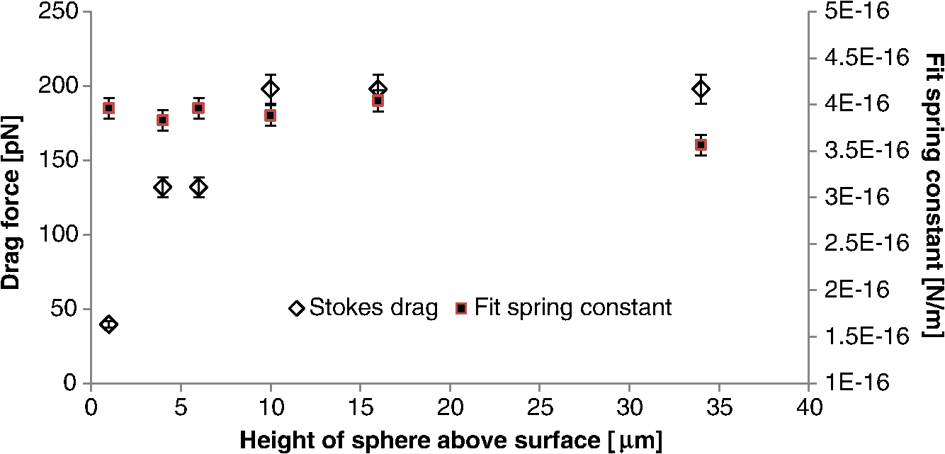 Next, we trapped a 1.98-μm-diameter microsphere in glycerol (Fisher Scientific, Pittsburgh, Pennsylvania). Glycerol is approximately 1000 times as viscous as PBS (), but because the MSD fit curve allows separate fitting of trap stiffness and viscous drag , the trap force can be distinguished from viscous drag. As seen in Fig. 7, the calibrated algorithm correctly measured the spring constant. Thus, we demonstrated that our calibration curve is not sensitive to variations in solvent viscosity. Fig. 7This graph shows the experimental results for the QPD algorithm calibration using microspheres ( for each data point) overlaid on results of our algorithm output for microsphere suspended in glycerol and our algorithm output for a trapped () Escherichia coli bacterium. The error bars correspond to measured uncertainty in (vertical) Stokes drag and (horizontal) results of our algorithm. 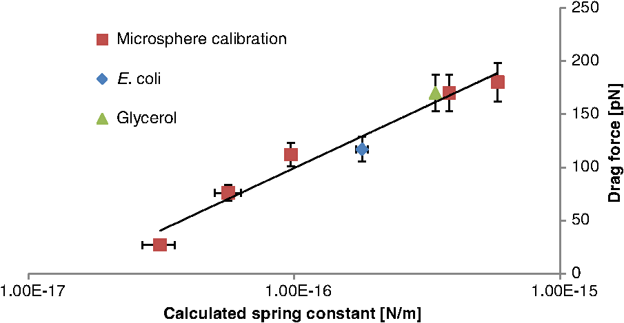 Additionally, because the objective lens is uncorrected for glycerol (at , , while ), the objective lens introduced wavefront aberrations (primarily spherical aberration) to the trapping beam. Thus, this measurement confirmed the results of test 1 and also demonstrated that our fitting algorithm does not require detailed information about the trapping beam wavefront. We next optically trapped a cylindrical object, a single E. coli bacterium. E. coli is a rod-shaped bacterium 1 μm in diameter and 3 μm in length. E. coli normally swim using a flagellum, so we first killed the bacteria with a brief exposure to intense ultraviolet light to avoid experimental artifacts. Once trapped, the bacterium oriented along the optical axis, and both QPD and Stokes drag measurements were performed. Critically important, the bacterium does not deform during the Stokes drag measurement. Modeling the bacterium as a cylinder of length and radius capped with hemispherical ends, the viscous drag at velocity (fluid density and viscosity ) is given by The first term results from the two hemispherical caps, and the second term is the drag force per unit length for a cylindrical object51 and contains Euler’s constant . Again, as seen in Fig. 7, the calibrated QPD algorithm correctly computed the spring constant, demonstrating that our algorithm results are insensitive to object shape. 5.Conclusion and Future WorkIn conclusion, we present a data acquisition and analysis toolkit based on particle tracking that allows near real-time measurements of the force applied by an optical trap to an object of unknown shape and composition. In addition, this analysis toolkit allows for a convenient calibration method for optical traps via the use of standard microspheres. This calibration step accurately calculates length-scale conversions, via diffusion constant ratios, as well as the effective strength of the trapping potential. Future work will be focused on applying the optical trap to a primary cilium, in an effort to measure the mechanical properties of this important organelle. AcknowledgmentsFunding for this work, provided by the National Institutes of Health under Grant R15DK092716, is gratefully acknowledged. ReferencesA. Resnick,
“Use of optical tweezers to probe epithelial mechanosensation,”
J. Biomed. Opt., 15
(1), 015005
(2010). http://dx.doi.org/10.1117/1.3316378 JBOPFO 1083-3668 Google Scholar
K. C. NeumanS. M. Block,
“Optical trapping,”
Rev. Sci. Instrum., 75
(9), 2787
–2809
(2004). http://dx.doi.org/10.1063/1.1785844 RSINAK 0034-6748 Google Scholar
J. A. Lock,
“Calculation of the radiation trapping force for laser tweezers by use of generalized Lorenz-Mie theory. II. On-axis trapping force,”
Appl. Opt., 43
(12), 2545
–2554
(2004). http://dx.doi.org/10.1364/AO.43.002545 APOPAI 0003-6935 Google Scholar
A. MazolliP. A. M. NetoH. M. Nussenzveig,
“Theory of trapping forces in optical tweezers,”
Proc. R. Soc. Lond. A Math. Phys. Eng. Sci., 459
(2040), 3021
–3041
(2003). http://dx.doi.org/10.1098/rspa.2003.1164 PRLAAZ 0080-4630 Google Scholar
N. B. Vianaet al.,
“Towards absolute calibration of optical tweezers,”
Phys. Rev. E Stat. Nonlin. Soft Matter Phys., 75
(2 Pt 1), 021914
(2007). http://dx.doi.org/10.1103/PhysRevE.75.021914 PLEEE8 1539-3755 Google Scholar
J. A. Lock,
“Calculation of the radiation trapping force for laser tweezers by use of generalized Lorenz-Mie theory. II. On-axis trapping force,”
Appl. Opt., 43
(12), 2545
–2554
(2004). http://dx.doi.org/10.1364/AO.43.002545 APOPAI 0003-6935 Google Scholar
W. H. WrightG. J. SonekM. W. Berns,
“Parametric study of the forces on microspheres held by optical tweezers,”
Appl. Opt., 33
(9), 1735
–1748
(1994). http://dx.doi.org/10.1364/AO.33.001735 APOPAI 0003-6935 Google Scholar
W. H. WrightG. J. SonekM. W. Berns,
“Radiation trapping forces on microspheres with optical tweezers,”
Appl. Phys. Lett., 63
(6), 715
–717
(1993). http://dx.doi.org/10.1063/1.109937 APPLAB 0003-6951 Google Scholar
Z. J. Liet al.,
“Calculation of radiation force and torque exerted on a uniaxial anisotropic sphere by an incident Gaussian beam with arbitrary propagation and polarization directions,”
Opt. Express, 20
(15), 16421
–16435
(2012). http://dx.doi.org/10.1364/OE.20.016421 OPEXFF 1094-4087 Google Scholar
A. AshkinJ. M. Dziedzic,
“Optical trapping and manipulation of viruses and bacteria,”
Science, 235
(4795), 1517
–1520
(1987). http://dx.doi.org/10.1126/science.3547653 SCIEAS 0036-8075 Google Scholar
C. Probstet al.,
“Microfluidic growth chambers with optical tweezers for full spatial single-cell control and analysis of evolving microbes,”
J. Microbiol. Methods, 95
(3), 470
–476
(2013). http://dx.doi.org/10.1016/j.mimet.2013.09.002 JMIMDQ 0167-7012 Google Scholar
H. XinC. ChengB. Li,
“Trapping and delivery of Escherichia coli in a microfluidic channel using an optical nanofiber,”
Nanoscale, 5
(15), 6720
–6724
(2013). http://dx.doi.org/10.1039/c3nr02088f 1556-276X Google Scholar
J. A. Lock,
“Scattering of a diagonally incident focused Gaussian beam by an infinitely long homogeneous circular cylinder,”
J. Opt. Soc. Am. A, 14
(3), 640
–652
(1997). http://dx.doi.org/10.1364/JOSAA.14.000640 JOAOD6 0740-3232 Google Scholar
T. M. GrzegorczykJ. A. Kong,
“Analytical expression of the force due to multiple TM plane-wave incidences on an infinite lossless dielectric circular cylinder of arbitrary size,”
J. Opt. Soc. Am. B, 24
(3), 644
–652
(2007). http://dx.doi.org/10.1364/JOSAB.24.000644 JOBPDE 0740-3224 Google Scholar
V. V. KotlyarA. G. Nalimov,
“Analytical expression for radiation forces on a dielectric cylinder illuminated by a cylindrical Gaussian beam,”
Opt. Express, 14
(13), 6316
–6321
(2006). http://dx.doi.org/10.1364/OE.14.006316 OPEXFF 1094-4087 Google Scholar
C. RockstuhlH. P. Herzig,
“Rigorous diffraction theory applied to the analysis of the optical force on elliptical nano- and micro-cylinders,”
J. Opt. A Pure Appl. Opt., 6
(10), 921
–931
(2004). http://dx.doi.org/10.1088/1464-4258/6/10/001 JOAOF8 1464-4258 Google Scholar
R. C. Gauthier,
“Theoretical investigation of the optical trapping force and torque on cylindrical micro-objects,”
J. Opt. Soc. Am. B, 14
(12), 3323
–3333
(1997). http://dx.doi.org/10.1364/JOSAB.14.003323 JOBPDE 0740-3224 Google Scholar
T. A. NieminenH. Rubinsztein-DunlopN. R. Heckenberg,
“Calculation and optical measurement of laser trapping forces on non-spherical particles,”
J. Quant. Spectrosc. Radiat., 70
(4–6), 627
–637
(2001). http://dx.doi.org/10.1016/S0022-4073(01)00034-6 JQSRAE 0022-4073 Google Scholar
A. G. Hoekstraet al.,
“Radiation forces in the discrete-dipole approximation,”
J. Opt. Soc. Am. A, 18
(8), 1944
–1953
(2001). http://dx.doi.org/10.1364/JOSAA.18.001944 JOAOD6 0740-3232 Google Scholar
L. Linget al.,
“Optical forces on arbitrary shaped particles in optical tweezers,”
J. Appl. Phys., 108
(7), 073110
(2010). http://dx.doi.org/10.1063/1.3484045 JAPIAU 0021-8979 Google Scholar
T. A. NieminenN. R. HeckenbergH. Rubinsztein-Dunlop,
“Computational modelling of optical tweezers,”
Proc. SPIE, 5514 514
–523
(2004). http://dx.doi.org/10.1117/12.557090 PSISDG 0277-786X Google Scholar
R. C. Gauthier,
“Computation of the optical trapping force using an FDTD based technique,”
Opt. Express, 13
(10), 3707
–3718
(2005). http://dx.doi.org/10.1364/OPEX.13.003707 OPEXFF 1094-4087 Google Scholar
K. Berg-SorensenH. Flyvbjerg,
“Power spectrum analysis for optical tweezers,”
Rev. Sci. Instrum., 75
(3), 594
–612
(2004). http://dx.doi.org/10.1063/1.1645654 RSINAK 0034-6748 Google Scholar
I. M. Tolic-NorrelykkeK. Berg-SorensenH. Flyvbjerg,
“MatLab program for precision calibration of optical tweezers,”
Comput. Phys. Commun., 159
(3), 225
–240
(2004). http://dx.doi.org/10.1016/j.cpc.2004.02.012 CPHCBZ 0010-4655 Google Scholar
H. Cabreraet al.,
“Experimental determination of trapping efficiency of optical tweezers,”
Philos. Mag. Lett., 93
(11), 655
–663
(2013). http://dx.doi.org/10.1080/09500839.2013.835078 PMLEEG 0950-0839 Google Scholar
D. BonessiK. BoninT. Walker,
“Optical forces on particles of arbitrary shape and size,”
J. Opt. A Pure Appl. Opt., 9
(8), S228
–S234
(2007). http://dx.doi.org/10.1088/1464-4258/9/8/S16 JOAOF8 1464-4258 Google Scholar
N. Malagninoet al.,
“Measurements of trapping efficiency and stiffness in optical tweezers,”
Opt. Commun., 214
(1–6), 15
–24
(2002). http://dx.doi.org/10.1016/S0030-4018(02)02119-3 OPCOB8 0030-4018 Google Scholar
L. P. GhislainN. A. SwitzW. W. Webb,
“Measurement of small forces using an optical trap,”
Rev. Sci. Instrum., 65
(9), 2762
–2768
(1994). http://dx.doi.org/10.1063/1.1144613 RSINAK 0034-6748 Google Scholar
P. BartlettD. Henderson,
“Three-dimensional force calibration of a single-beam optical gradient trap,”
J. Phys. Condens. Matter, 14
(33), 7757
–7768
(2002). http://dx.doi.org/10.1088/0953-8984/14/33/314 JCOMEL 0953-8984 Google Scholar
J. K. DreyerK. Berg-SorensenL. Oddershede,
“Improved axial position detection in optical tweezers measurements,”
Appl. Opt., 43
(10), 1991
–1995
(2004). http://dx.doi.org/10.1364/AO.43.001991 APOPAI 0003-6935 Google Scholar
S. KimB. D. Dynlacht,
“Assembling a primary cilium,”
Curr. Opin. Cell Biol., 25
(4), 506
–511
(2013). http://dx.doi.org/10.1016/j.ceb.2013.04.011 COCBE3 0955-0674 Google Scholar
G. G. Germino,
“Linking cilia to Wnts,”
Nat. Genet., 37
(5), 455
–457
(2005). http://dx.doi.org/10.1038/ng0505-455 NGENEC 1061-4036 Google Scholar
M. A. LancasterJ. G. Gleeson,
“The primary cilium as a cellular signaling center: lessons from disease,”
Curr. Opin. Genet. Dev., 19
(3), 220
–229
(2009). http://dx.doi.org/10.1016/j.gde.2009.04.008 COGDET 0959-437X Google Scholar
W. Liuet al.,
“Mechanoregulation of intracellular concentration is attenuated in collecting duct of monocilium-impaired orpk mice,”
Am. J. Physiol., 289
(5), F978
–F988
(2005). http://dx.doi.org/10.1152/ajprenal.00260.2004 AJPHAP 0002-9513 Google Scholar
S. H. Lowet al.,
“Polycystin-1, STAT6, and P100 function in a pathway that transduces ciliary mechanosensation and is activated in polycystic kidney disease,”
Dev. Cell, 10
(1), 57
–69
(2006). http://dx.doi.org/10.1016/j.devcel.2005.12.005 1534-5807 Google Scholar
S. Mukhopadhyayet al.,
“The ciliary G-protein-coupled receptor Gpr161 negatively regulates the sonic Hedgehog pathway via cAMP signaling,”
Cell, 152
(1–2), 210
–223
(2013). http://dx.doi.org/10.1016/j.cell.2012.12.026 CELLB5 0092-8674 Google Scholar
S. M. Nauliet al.,
“Polycystins 1 and 2 mediate mechanosensation in the primary cilium of kidney cells,”
Nat. Genet., 33
(2), 129
–137
(2003). http://dx.doi.org/10.1038/ng1076 NGENEC 1061-4036 Google Scholar
S. M. NauliJ. Zhou,
“Polycystins and mechanosensation in renal and nodal cilia,”
Bioessays, 26
(8), 844
–856
(2004). http://dx.doi.org/10.1002/(ISSN)1521-1878 BIOEEJ 0265-9247 Google Scholar
C. Ottet al.,
“Primary cilia utilize glycoprotein-dependent adhesion mechanisms to stabilize long-lasting cilia-cilia contacts,”
Cilia, 1
(1), 1
–14
(2012). http://dx.doi.org/10.1186/2046-2530-1-3 2046-2530 Google Scholar
L. M. Satlinet al.,
“Epithelial Na(+) channels are regulated by flow,”
Am. J. Physiol., 280
(6), F1010
–F1018
(2001). AJPHAP 0002-9513 Google Scholar
L. Schneideret al.,
“Directional cell migration and chemotaxis in wound healing response to PDGF-AA are coordinated by the primary cilium in fibroblasts,”
Cell Physiol. Biochem., 25
(2–3), 279
–292
(2010). http://dx.doi.org/10.1159/000276562 CEPBEW 1015-8987 Google Scholar
L. Schneideret al.,
“The Na+/H+ exchanger NHE1 is required for directional migration stimulated via PDGFR-alpha in the primary cilium,”
J. Cell Biol., 185
(1), 163
–176
(2009). http://dx.doi.org/10.1083/jcb.200806019 JCLBA3 0021-9525 Google Scholar
J. M. Shillingfordet al.,
“The mTOR pathway is regulated by polycystin-1, and its inhibition reverses renal cystogenesis in polycystic kidney disease,”
Proc. Natl. Acad. Sci. U. S. A., 103
(14), 5466
–5471
(2006). http://dx.doi.org/10.1073/pnas.0509694103 PNASA6 0027-8424 Google Scholar
T. WatnickG. Germino,
“From cilia to cyst,”
Nat. Genet., 34
(4), 355
–356
(2003). http://dx.doi.org/10.1038/ng0803-355 NGENEC 1061-4036 Google Scholar
T. Weimbs,
“Polycystic kidney disease and renal injury repair: common pathways, fluid flow, and the function of polycystin-1,”
Am. J. Physiol., 293
(5), F1423
–F1432
(2007). AJPHAP 0002-9513 Google Scholar
M. E. WernerB. J. Mitchell,
“Planar cell polarity: microtubules make the connection with cilia,”
Curr. Biol., 22
(23), R1001
–R1004
(2012). http://dx.doi.org/10.1016/j.cub.2012.10.030 CUBLE2 0960-9822 Google Scholar
S. Yuanet al.,
“Target-of-rapamycin complex 1 (Torc1) signaling modulates cilia size and function through protein synthesis regulation,”
Proc. Natl. Acad. Sci. U. S. A., 109
(6), 2021
–2026
(2012). http://dx.doi.org/10.1073/pnas.1112834109 PNASA6 0027-8424 Google Scholar
J. SavigeS. RatnaikeD. Colville,
“Retinal abnormalities characteristic of inherited renal disease,”
J. Am. Soc. Nephrol., 22
(8), 1403
–1415
(2011). http://dx.doi.org/10.1681/ASN.2010090965 JASNEU 1046-6673 Google Scholar
H. Takeuchiet al.,
“Mechanism of olfactory masking in the sensory cilia,”
J. Gen. Physiol., 133
(6), 583
–601
(2009). http://dx.doi.org/10.1085/jgp.200810085 JGPLAD 0022-1295 Google Scholar
D. R. RichA. L. Clark,
“Chondrocyte primary cilia shorten in response to osmotic challenge and are sites for endocytosis,”
Osteoarthr. Cartil., 20
(8), 923
–930
(2012). http://dx.doi.org/10.1016/j.joca.2012.04.017 OSCAEO 1063-4584 Google Scholar
A. ResnickU. Hopfer,
“Force-response considerations in ciliary mechanosensation,”
Biophys. J., 93
(4), 1380
–1390
(2007). http://dx.doi.org/10.1529/biophysj.107.105007 BIOJAU 0006-3495 Google Scholar
A. ResnickU. Hopfer,
“Mechanical stimulation of primary cilia,”
Front. Biosci., 13
(1), 1665
–1680
(2008). http://dx.doi.org/10.2741/2790 1093-9946 Google Scholar
H. Higginbothamet al.,
“Arl13b in primary cilia regulates the migration and placement of interneurons in the developing cerebral cortex,”
Dev. Cell, 23
(5), 925
–938
(2012). http://dx.doi.org/10.1016/j.devcel.2012.09.019 1534-5807 Google Scholar
D. Daiet al.,
“Planar cell polarity effector gene Intu regulates cell fate-specific differentiation of keratinocytes through the primary cilia,”
Cell Death Differ., 20
(1), 130
–138
(2013). http://dx.doi.org/10.1038/cdd.2012.104 1350-9047 Google Scholar
M. DeinerS. L. TammS. Tamm,
“Mechanical properties of ciliary axonemes and membranes as shown by paddle cilia,”
J. Cell Sci., 104
(Pt 4), 1251
–1262
(1993). JNCSAI 0021-9533 Google Scholar
E. A. Schwartzet al.,
“Analysis and modeling of the primary cilium bending response to fluid shear,”
Am. J. Physiol., 272
(1 Pt 2), F132
–F138
(1997). AJPHAP 0002-9513 Google Scholar
C. J. Brokaw,
“Is the pattern of flagellar and ciliary axonemes an efficient arrangement for generating planar bending?,”
J. Mechanochem. Cell Motil., 4
(2), 101
–111
(1977). JMCLAO 0091-6552 Google Scholar
C. J. Brokaw,
“Computer simulation of flagellar movement VIII: coordination of dynein by local curvature control can generate helical bending waves,”
Cell Motil. Cytoskeleton, 53
(2), 103
–124
(2002). http://dx.doi.org/10.1002/(ISSN)1097-0169 CMCYEO 0886-1544 Google Scholar
C. B. Lindemann,
“A model of flagellar and ciliary functioning which uses the forces transverse to the axoneme as the regulator of dynein activation,”
Cell Motil. Cytoskeleton, 29
(2), 141
–154
(1994). http://dx.doi.org/10.1002/(ISSN)1097-0169 CMCYEO 0886-1544 Google Scholar
K. A. Schmitzet al.,
“Measurement of the force produced by an intact bull sperm flagellum in isometric arrest and estimation of the dynein stall force,”
Biophys. J., 79
(1), 468
–478
(2000). http://dx.doi.org/10.1016/S0006-3495(00)76308-9 BIOJAU 0006-3495 Google Scholar
A. Resnick,
“Design and construction of a space-borne optical tweezer apparatus,”
Rev. Sci. Instrum., 72
(11), 4059
–4065
(2001). http://dx.doi.org/10.1063/1.1406921 RSINAK 0034-6748 Google Scholar
A. Resnick,
“Use of optical tweezers for colloid science,”
J. Colloid Interface Sci., 262
(1), 55
–59
(2003). http://dx.doi.org/10.1016/S0021-9797(03)00193-0 JCISA5 0021-9797 Google Scholar
M. J. Saxton,
“Single-particle tracking: the distribution of diffusion coefficients,”
Biophys. J., 72
(4), 1744
–1753
(1997). http://dx.doi.org/10.1016/S0006-3495(97)78820-9 BIOJAU 0006-3495 Google Scholar
T. C. LiM. G. Raizen,
“Brownian motion at short time scales,”
Ann. Phys. Berlin, 525
(4), 281
–295
(2013). http://dx.doi.org/10.1002/andp.v525.4 ANPYA2 0003-3804 Google Scholar
G. VolpeG. Volpe,
“Simulation of a Brownian particle in an optical trap,”
Am. J. Phys., 81
(3), 224
–230
(2013). http://dx.doi.org/10.1119/1.4772632 AJPIAS 0002-9505 Google Scholar
J. Glaser,
“Simulation for Brownian Motion within an Harmonic Potential,”
(2013) http://www.mathworks.com/matlabcentral/fileexchange/44733 December ). 2013). Google Scholar
H. Faxén, Der Widerstand gegen die Bewegung einer starren Kugel in einer zähen Flüssigkeit, die zwischen zwei parallelen ebenen Wänden eingeschlossen ist [Mitteilg 1], Almquist & Wiksells Boktryckeri-A.-B., Stockholm
(1924). Google Scholar
P. SharmaS. GhoshS. Bhattacharya,
“high-precision study of hindered diffusion near a wall,”
Appl. Phys. Lett., 97
(10), 104101
(2010). http://dx.doi.org/10.1063/1.3486123 APPLAB 0003-6951 Google Scholar
BiographyJoseph Glaser received his BS degree in physics from Cleveland State University in 2014 and is currently enrolled in the physics graduate program at Drexel University. David Hoeprich received his MS degree in medical physics from Cleveland State University in 2012. He is currently employed as a board-certified medical physicist at Applied Medical Physics In Radiology, Inc., located in Kirtland Hills, Ohio. Andrew Resnick is an assistant professor at Cleveland State University. He received his BS degree in physics from Rensselaer Polytechnic Institute in 1991 and his PhD degree in physics from the University of Alabama in Huntsville in 1996. His current research interests include cellular mechanotransduction and microscopy. He is a member of the American Physical Society, American Physiological Society, and Optical Society of America. |