1.

Introduction

The development of optical technology has increased the requirements for high-precision optical elements, especially aspheric optics. When used in an optical system, aspheric optics can increase the degrees of freedom in a design, reduce the weight and size of the system, and provide a significant advantage for correcting system aberrations.¹

The polishing procedure is vital for acquiring high-accuracy aspheric optics during the manufacturing process. The traditional polishing process, which depends on skilled workers, does not meet current needs, due to its inefficiency, unpredictability, and so on. Hence, various computer-controlled optical surfacing (CCOS) processes have been developed in recent decades.^2–6 CCOS adopting a small-pitch tool was first developed by Jones,² and it has been successfully used for polishing various types of optical elements.^7,8 Its form correction efficiency is much higher than the artisanal processes. But, there is a mismatch between the pitch tool and the work-piece surface when polishing the aspheric optics. Therefore, some other polishing technologies were developed, including noncontact polishing, e.g., ion beam figuring (IBF)⁹ and cabrasive jet polishing;^10,11 contact polishing using flexible or semiflexible polishing tools, e.g., magnetorheological finishing (MRF),^12,13 bonnet tool polishing,^14–16 and rigid conformal lap polishing.⁶ The bonnet polishing technology was first developed by Zeeko, Ltd. (Leicestershire, United Kingdom) in collaboration with the Optical Science Laboratory at the University College London and Loh Optikmaschinen.^17,18 This technology uses a rotating inflated spherical membrane tool (the “bonnet”) that naturally molds itself to the local aspheric surface and maintains stability to provide natural smoothing. Compared to other polishing processes, the bonnet shows higher removal efficiency, no mismatch between the work-piece and the tool, and the ability to control the mirror’s edges.^5,19–22 Bonnets have thus been widely used for polishing optical lenses, especially aspheric optics,²³ molds,²⁴ freeform surfaces,²⁵ structured surfaces,²⁶ and so on.

In bonnet tool polishing, much attention has been paid to the tool influence function (TIF),^14,27,28 the edge effect,^21,22 the final surface error,^5,19 and so on. However, little attention has been paid to the surface residual error induced by the superposition of the TIF. These residual errors, including some medium-high frequency errors, are severe in some applications, such as intense laser systems and high resolution image formation systems.^29,30 Different TIFs will cause different surface residual errors. Hence, research on the effect of different polishing parameters on the residual error is significant for the purpose of achieving extremely high surface accuracy.

In this paper, the residual error induced by the superposition of the TIF is first theoretically presented. Then, practical and simulation experiments to study the effect of various polishing parameters on the residual error using the minimum residual error method are described. Finally, an optimal combination of these parameters is determined and verified.

2.

Theoretical Background

2.1.

TIF Model

Bonnet polishing adopts a unique precession motion, leading to a Gaussian-like TIF²⁷ as shown in Fig. 1. According to the well-known Preston’s law,³¹ the material removal function can be expressed as

Eq. (1)

$$\frac{dz}{dt}=kpv,$$

where $dt$ is the dwell time, $dz$ is the material removal during the dwell time, $k$ is the removal coefficient, $p$ is the polishing pressure, and $v$ is the relative speed between the tool and the work-piece. There are several TIF models of bonnet polishing. For example, Kim and Kim³² proposed a static tool influence function (sTIF). Li et al.²⁷ presented simulation results of static and dynamic TIFs. Wang et al.²⁸ demonstrated and modeled three kinds of static TIFs based on the finite element analysis method. As in the practical polishing process in which the four discrete precession polishing modes¹⁴ are usually adopted and the rotation speed of $A$-axis is zero, the four discrete precession static tool influence function (${\mathrm{sTIF}}_{\mathrm{d}}$) should be used in the simulation polishing process to make the simulation closer to the actual.

Fig. 1

Tool influence function (TIF) for bonnet polishing: (a) contour map of TIF and (b) section profile of TIF. (Polishing parameters: bonnet radius is 80 mm, 5.54% ${\mathrm{CeO}}_2$ weight percentage polishing slurry is used, the rotation speed of $H$-axis ${\omega }_1=500\mathrm{rpm}$, the rotation speed of $A$-axis ${\omega }_2=20\mathrm{rpm}$, $\text{inner pressure}=0.25\mathrm{MPa}$, $z$ $\text{offset}=0.8\mathrm{mm}$, $\text{precession angle}=25\mathrm{deg}$, and the dwell time is 6 s).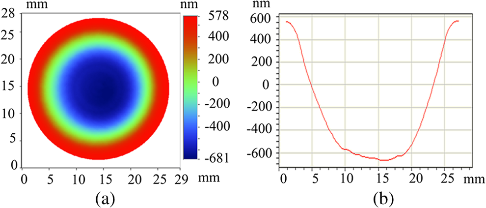

Without loss of generality, the TIF of bonnet polishing is mostly modeled on a flat surface.^27,28,32 Figure 2 demonstrates the schematic diagram of the discrete precession bonnet polishing. Figure 2(a) shows the tool polishing a flat surface following a raster path, and Fig. 2(b) presents the detailed geometry of bonnet tool polishing a flat surface. Here, $Q$ is a point in the contact area, ${\omega }_1$ is the rotation speed of the $H$-axis, $v_r$ is the velocity of point $Q$ derived from the rotation about the $H$-axis, ${\omega }_2$ is the rotation speed of the $A$-axis, $v_p$ is the velocity of point $Q$ derived from the rotation about the $A$-axis, $O_1$ is the center of the bonnet tool, $O_2$ is the center of the contact area, $l$ is the $z$ offset of the bonnet, $R_0$ is the radius of the bonnet tool, and $\alpha$ is the precession angle.

Fig. 2

Schematic diagram of the discrete precession bonnet polishing: (a) bonnet tool polishing a flat surface following the raster path and (b) detailed geometry of bonnet tool polishing a flat surface.

${\mathrm{sTIF}}_{\mathrm{d}}$ ($x,y$) can be expressed as²⁸

Eq. (2)

$${\mathrm{sTIF}}_{\mathrm{d}}(x,y)=\sum _{i=1}^4\{{\mathrm{\Delta }}_i\frac{T}{4}k{p}_{\max }{\left[\exp \right(-\frac{(x^2+y^2)}{2{\sigma }^2}\left)\right]}^{\phi }\sqrt{{\{|{\mathit{\omega }}_1|[(R_0-l)\sin \alpha -y\cos \alpha ]\}}^2+{(|{\mathit{\omega }}_1|\cos \alpha )}^2{x}^2}\},$$

where $p_{\max }$ is the maximum pressure in the contact area, $\sigma$ is the standard deviation of the pressure distribution, $\phi$ is the modification coefficient, $T$ is the unit dwell time, and ${\mathrm{\Delta }}_i$ is the matrix of the velocity direction of each step. Assuming that the initial velocity direction angle is zero, the velocity direction angle of the $i$’th step, ${\theta }_i$, can be expressed in degrees as

Eq. (3)

$${\theta }_i=(i-1)·90\mathrm{deg}\mathrm{.}$$

Therefore, ${\mathrm{\Delta }}_i$ can be easily derived using a MATLAB code when we know the value of ${\theta }_i$. Using the aforementioned equations, we can easily simulate ${\mathrm{sTIF}}_{\mathrm{d}}$ under different conditions. Figure 3 shows the simulation results of ${\mathrm{sTIF}}_{\mathrm{d}}$, which is a Gaussian-like shape. Figure 3(a) shows the three-dimensional contour of ${\mathrm{sTIF}}_{\mathrm{d}}$, and Fig. 3(b) shows its $x/y$ section profile. It is completely axisymmetric as shown in Fig. 3(b) that its two section profiles are exactly coincidence.

Fig. 3

Simulation results for ${\mathrm{sTIF}}_{\mathrm{d}}$: (a) three-dimensional contour of simulated ${\mathrm{sTIF}}_{\mathrm{d}}$, and (b) $x/y$ section profile of simulated ${\mathrm{sTIF}}_{\mathrm{d}}$. (Polishing parameters: bonnet radius is 80 mm, $k{=-2.4059\times 10}^{-13}$, ${\omega }_1=500\mathrm{rpm}$, $\text{inner pressure}=0.25\mathrm{MPa}$, $z$ $\text{offset}=0.8\mathrm{mm}$, $\text{precession angle}=25\mathrm{deg}$, and the dwell time is 12 s).

2.2.

Residual Error Induced by the Superposition of TIF

Bonnet polishing is a type of deterministic polishing. The amount of material removed in bonnet polishing, $H(x,y)$, is equal to the two-dimensional (2-D) convolution between the material removal function per unit time $R(x,y)$ and the dwell time function $D(x,y)$, along with the motion track:^33,34

Eq. (4)

$$H(x,y)=R(x,y)**D(x,y).$$

The convolution between $R(x,y)$ and $D(x,y)$ leads to the residual error caused by the superposition of $R(x,y)$ (hereafter called “residual error” for brevity). Therefore, the residual error $E(x,y)$ after the polishing process can be expressed as

Eq. (5)

$$E(x,y)=H_0(x,y)-R(x,y)**D(x,y),$$

where $H_0(x,y)$ is the amount of material to be removed.

In order to demonstrate the residual error theoretically, a material removal experiment was simulated. Table 1 lists the simulation parameters. The material depth to be removed was $1\mu \mathrm{m}$. A raster path was adopted, and the distance between adjacent points was 2 mm in both the $x$ and the $y$ directions. Two-dimensional simulation results are shown in Fig. 4. In Fig. 4, the principle of residual error generation is demonstrated. Omitting the edge effect, the peak-to-valley value (PV) of the residual error is 18.98 nm. Therefore, research for minimizing the residual error would be quite valuable for achieving extremely accurate optical surfaces.

Table 1

Simulation parameters.

Parameters	Value
Bonnet tool radius (mm)	80
Inner pressure (MPa)	0.15
$z$ offset (mm)	0.8
$H$-axis speed (rpm)	500
Precession angle (deg)	16
Distance between dwell points (mm)	2

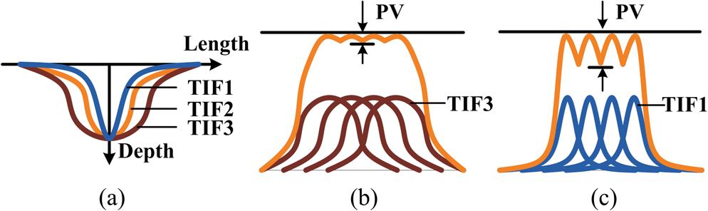
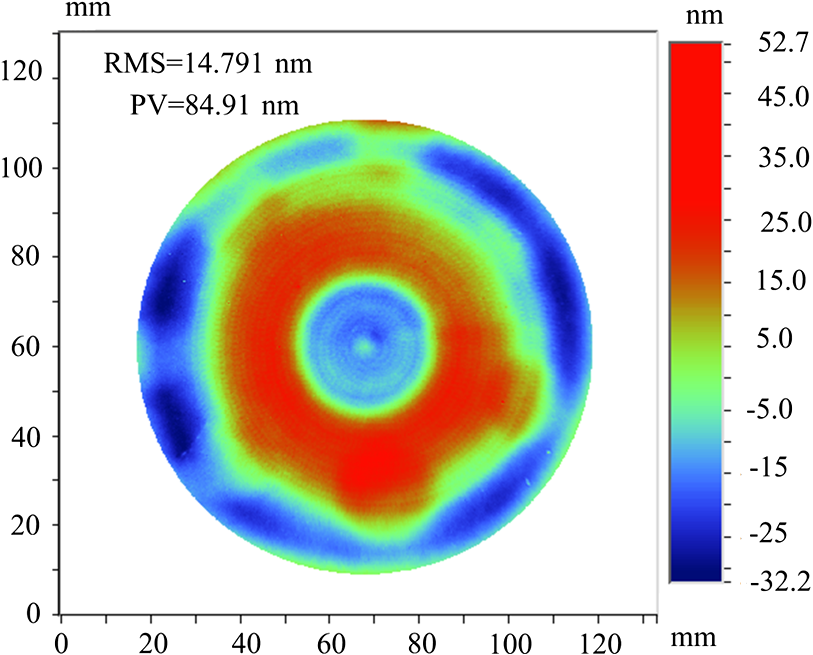
Fig. 4

Simulation results of the material removal. [The symbols in this figure correspond to Eqs. (4) and (5).]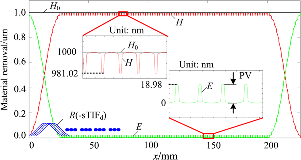

It has been reported that this residual error is mainly affected by the raster interval and the size of TIF.³⁵ However, as shown in Fig. 5, different shapes of TIF may also have effects to it, even though they have the same size. Figure 5(a) shows three different shapes of TIF with the same size and the maximum removal rate, Fig. 5(b) shows the material removal generated by the superposition of TIF3, and Fig. 5(c) shows the material removal generated by the superposition of TIF1. It is noted that the PV value of the residual error using TIF3 is smaller than that using TIF1 when the raster intervals of them are the same. The shape of TIF in bonnet polishing is influenced by many factors, such as inner pressure, precession angle, $z$ offset, and so on. Hence, it is necessary to study these factors’ effect to the residual error and determine an optimal combination of them to produce a surface with minimum residual error.

Fig. 5

A schematic diagram to show the effects of TIF shape to the residual error: (a) three different shapes of TIF with the same size and the maximum removal rate, (b) material removal generated by the superposition of TIF3, and (c) material removal generated by the superposition of TIF1.

3.

Experimental Analysis of the Effect of Polishing Parameters on Residual Error

There are two modes of bonnet polishing tool motion: the discrete dwell point (DDP) mode and the continuous dwell point (CDP) mode. In the DDP mode, the tool dwells at each point for a designated time and then moves to another dwell point and repeats the cycle. For a raster path, this mode will lead to the aforementioned residual error in the $x$ and the $y$ directions. In the CDP mode, the dwell time at each point is converted into an average speed in the interval between each point, and different dwell times at different dwell points are obtained by controlling the speed between in each interval. The CDP mode can eliminate the residual error induced by the superposition of TIF in one direction and reduce feeding time between each dwell point compared with the DDP mode. However, a residual error remains in the raster space direction.

3.1.

Residual Error Induced by the Superposition of TIF

We conducted a uniform removal experiment with our newly developed experimental prototype. The prototype is shown in Fig. 6. The experiment was conducted on a plane 100-mm-diameter BK7 glass with a surface polished to 84.91-nm PV. Figure 7 shows the initial surface error of the work-piece measured through QED SSI® (QED Optics, Rochester, New York). In order to retain unpolished surfaces from which the absolute removal depth could be established, an 80-mm-diameter subarea of the part was polished. A raster path in the CDP mode was used with a raster distance of 3 mm. ${\mathrm{CeO}}_2$ polishing slurry is used with the weight percentage of 1.96% in this experiment. Table 2 lists the other experimental conditions.

Fig. 6

Experimental prototype for bonnet polishing.

Fig. 7

Initial surface error of the BK7 part.

Table 2

Uniform removal conditions.

Parameters	Value
Tool radius (mm)	80
Precession angle (deg)	23
$H$-axis speed (rpm)	500
Feed speed ($\mathrm{mm}/\min$)	600
$z$ offset (mm)	0.7
Inner pressure (MPa)	0.25
Total polishing time (min)	24

Figure 8 shows the measured results of the surface profile after uniform removal from QED SSI®, and they are processed using WYKO VISION software for optical testing (Developed by Veeco Instruments Inc., New York). Figure 8(a) shows the whole surface and the partially enlarged surface contour; the sectional profiles along the $x$ and the $y$ directions are shown in Fig. 8(b). The residual error appears to be in the $x$ direction. The surface profile in the $y$ direction is obviously tilted. This could be traced to a tilt in the work-piece on the machine. Also, omitting the tilted error, there is also fluctuation in this direction, which may be induced by the “stick-slip” phenomenon during the polishing process. As shown in the top part of Fig. 8(b), the PV of the induced residual error is $\sim 40\mathrm{nm}$, but it is not constant over the entire surface. It could be caused by the initial surface not being flat enough as shown in Fig. 7. Other reasons, such as the instability of TIF, could also induce that. Therefore, the residual error generated by the actual polishing process includes many other errors and not just the residual error aforementioned induced by the superposition of the TIF. Viewing this, the practical experiments could not generate this residual error accurately and could not be used to analyze the effects of the factors to the residual error. Three main reasons have been concluded as follows:

• 1. The initial surface profile is not a standard plane surface, which leads to different tool removal at each dwell point.

• 2. The instability of the TIF as induced by fluctuations of slurry weight percentage, etc., leads to different tool removal at each dwell point.

• 3. The error induced by holding the work-piece and the accuracy of the machine would make the work-piece tilt as shown in Fig. 8.

Fig. 8

Work-piece surface profile after uniform removal: (a) Surface contour after uniform polishing and (b) $x$ and $y$ profile of the partial surface as shown in (a).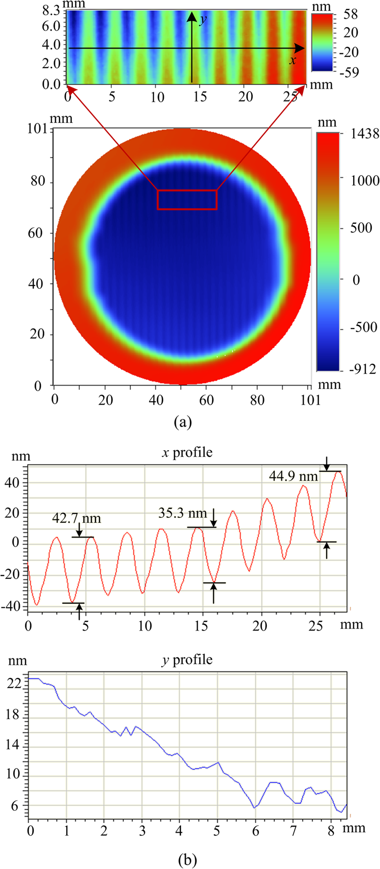

Hence, simulation experiments were adopted for this analysis. The simulation analyzes the effects of only the polishing parameters on the residual error and can exclude other uncorrelated parameters.

3.2.

Simulation Experiment

3.2.1.

Experimental design

Several parameters affect the surface residual error in the bonnet polishing process as mentioned above. On both the lab scale and the industrial scale, it can be extremely time consuming and expensive to run a large number of experiments to test the influence and the combinations of all parameters in a practical polishing process. Hence, a judicious experimental design is necessary, especially for a multiparameter bonnet polishing process. This can not only simplify and standardize experimental operations but also will permit identification of critical parameters and optimization of their combinations to minimize residual error. Therefore, orthogonal experiment design was used in this study.

Considering the minimum residual error method, the PV of the residual error was chosen as the quality characteristic for the orthogonal experiment design, and the minimized PV will indicate the smallest residual error in this study. In the bonnet polishing process, parameters, such as inner pressure, $z$ offset, $H$-axis speed, precession angle, and raster distance, are the major operating parameters that influence the residual error. In this study, raster distance defines the space between each feeding line in a raster path as demonstrated in Fig. 2(b). It can be easily noted that the best value of $z$ offset and raster distance for a polishing process is directly influenced by the size of the bonnet tool. Therefore, the following two ratios defining the relationship between $z$ offset, raster distance, and bonnet tool radius are used to replace $z$ offset and raster distance in the experiment.

Eq. (6)

$${\eta }_{z\text{offset}}=\frac{z\text{offset}}{R_0},$$

Eq. (7)

$${\eta }_{\text{raster distance}}=\frac{\text{raster distance}}{R_0}.$$

The bonnet tool radius is defined as 80 mm in this experiment. An orthogonal experiment design for these five parameters at four levels was used to evaluate their impact on the multiparameter bonnet polishing process, as summarized in Table 3. The four levels for each parameter are within the commonly used ranges for bonnet tool polishing.

Table 3

Parameters and levels of orthogonal experiment design.

Parameter	Level
	1	2	3	4
Inner pressure (MPa)	0.10	0.15	0.20	0.25
${\eta }_{z\text{offset}}$	0.0025	0.005	0.0075	0.01
${\eta }_{\text{raster distance}}$	0.0125	0.01875	0.025	0.03125
$H$-axis speed (rpm)	250	500	750	1000
Precession angle (deg)	16	19	22	25

The orthogonal experiment designs are expressed using the notation $Ln$ ($t^k$), where $L$ is the symbol of the orthogonal layout; $n$ indicates the number of experiments instead of the full factorial experiments; $t$ is the number of levels of each factor investigated, and $k$ is the number of factors investigated. Therefore, the orthogonal array employed for this study was the $L16$ ($4^5$) array, where the experiment requires only 16 runs rather than the 1024 runs that would be required for the full $4^5$ factorial experiment. Details of the $L16$ ($4^5$) orthogonal array are summarized in Table 4. The numbers 1, 2, 3, and 4 denote the four levels for the five control parameters. Each row of Table 4 represents a run for each of the five parameters and is specified at one of the four levels.

Table 4

Experimental layout using an L16 (45) orthogonal array.

Experiment number	Parameters
	Inner pressure	$z$ offset	Raster distance	$H$-axis speed	Precession angle
1	1	1	1	1	1
2	1	2	2	2	2
3	1	3	3	3	3
4	1	4	4	4	4
5	2	1	2	3	4
6	2	2	1	4	3
7	2	3	4	1	2
8	2	4	3	2	1
9	3	1	3	4	2
10	3	2	4	3	1
11	3	3	1	2	4
12	3	4	2	1	3
13	4	1	4	2	3
14	4	2	3	1	4
15	4	3	2	4	1
16	4	4	1	3	2

3.2.2.

Experimental procedure

Figure 9 demonstrates the flowchart of each simulation procedure in the orthogonal experiment. First, each ${\mathrm{sTIF}}_{\mathrm{d}}$ using the parameters of each row in Table 4 was modeled and simulated by applying Eq. (2). The uniform material removal could then be simulated using Eq. (4) on a standard plane surface, and a $5\text{-}\mu \mathrm{m}$ depth of material was defined as the amount of material to be removed for each experiment without loss of generality. After that, the final surface error could be determined by using Eq. (5). The PV of the residual error was calculated based on the data for the central part of the uniform removal area, without consideration of the edge zone.

Fig. 9

Flowchart of each simulation procedure in the orthogonal experiment.

3.2.3.

Orthogonal experiment results

The results of the orthogonal experiment are summarized in Table 5. The average PV of the residual error for the 16 experiments can be determined from the data listed in Table 5 and is given by the following expression.

Eq. (6)

$$Y=\frac{1}{16}\sum _1^{16}{y}_i=92.6,$$

where $y_i$ is the PV of the residual error of the $i$’th experiment run. In orthogonal experiment design, the average result at each level for a particular parameter can indicate its influence at that level. Hence, through analysis of the average results for each parameter, information can be obtained on how each parameter affects the surface residual error. For example, the first four runs for the inner pressure were conducted at 0.1 MPa (level 1). Hence, these four runs should belong to one subgroup for this parameter. Runs 5 through 8, 9 through 12, and 13 through 16 belong to the other three subgroups for levels 2, 3, and 4, respectively. The average values ($\overline{I_1}$, $\overline{I_2}$, $\overline{I_3}$, $\overline{I_4}$) can be calculated for each subgroup. For level 1 of the inner pressure, $\overline{I_1}$ is 72.5 nm. The resulting values for the four subgroups for each of the five control parameters are listed in Table 5.

Table 5

Orthogonal experiment results and calculated average responses.

Experiment number	Parameters					PV of residual error (nm)
	Inner pressure (MPa)	${\eta }_{z\text{offset}}$	${\eta }_{\text{raster distance}}$	$H$-axis speed (rpm)	Precession angle (deg)
1	0.10	0.0025	0.0125	250	16	54.7
2	0.10	0.005	0.01875	500	19	65.7
3	0.10	0.0075	0.025	750	22	75.3
4	0.10	0.01	0.03125	1000	25	94.4
5	0.15	0.0025	0.01875	750	25	115.8
6	0.15	0.005	0.0125	1000	22	45.1
7	0.15	0.0075	0.03125	250	19	121.8
8	0.15	0.01	0.025	500	16	94.9
9	0.20	0.0025	0.025	1000	19	140.7
10	0.20	0.005	0.03125	750	16	130.0
11	0.20	0.0075	0.0125	500	25	48.8
12	0.20	0.01	0.01875	250	22	60.2
13	0.25	0.0025	0.03125	500	22	214.6
14	0.25	0.005	0.025	250	25	98.8
15	0.25	0.0075	0.01875	1000	16	75.0
16	0.25	0.01	0.0125	750	19	45.4
$\overline{I_1}$	72.5	131.5	48.5	83.9	88.7	$Y=92.6$
$\overline{I_2}$	94.4	84.9	79.2	106.0	93.4
$\overline{I_3}$	94.9	80.2	102.4	91.7	98.8
$\overline{I_4}$	108.5	73.7	140.2	88.8	89.5

3.2.4.

Discussion

The influence of each parameter on the residual error can be assessed by comparing the average PV of residual error for each level ($\overline{I_1}$, $\overline{I_2}$, $\overline{I_3}$, $\overline{I_4}$) in graphical form, as shown in Fig. 10. As shown in Fig. 10(a), the effect of the inner pressure on the residual error is weak, but increasing the inner pressure would lead to an increase in the residual error. From Fig. 10(b), we can see that a larger $z$ offset would give a smaller residual error. The PV of the residual error shows a monotonic increase with increasing raster distance as demonstrated in Fig. 10(c). Both the $H$-axis speed and the precession angle have little impact on the PV of the surface residual error as shown in Figs. 10(d) and 10(e). However, we still can determine the best-fitted $H$-axis speed and precession angle to achieve the approximate minimum residual error.

Fig. 10

Effects of parameters on the peak-to-valley value (PV) of the surface residual error: (a) effect of the inner pressure on the residual error, (b) effect of the $z$ offset on the residual error, (c) effect of the raster distance on the residual error, (d) effect of the $H$-axis speed on the residual error, and (e) effect of the precession angle on the residual error.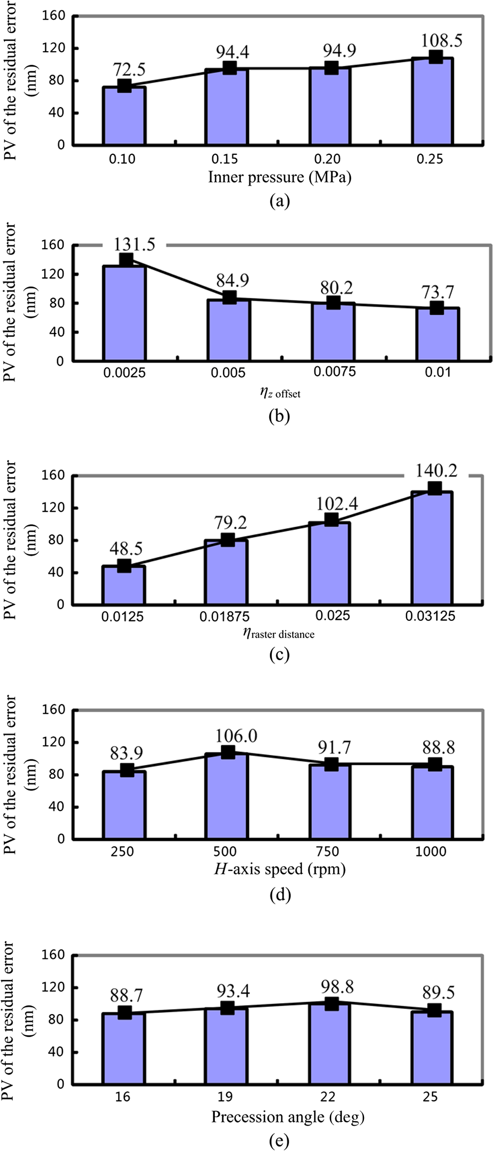

In summary, in terms of impact on the residual error, the parameters considered here rank as follows, from most to least significant: raster distance, $z$ offset, inner pressure, $H$-axis speed, and precession angle. In order to achieve the minimum residual error, the raster distance and the inner pressure should be relatively small and the $z$ offset should be relatively large. Moreover, there exist optimal values of the $H$-axis speed and the precession angle to achieve the minimum residual error. Hence, the optimal combination of the polishing parameter values can be easily deduced, as listed in Table 6.

Table 6

Optimal combination of polishing parameter values.

Parameters	Value
Bonnet radius (mm)	80
Inner pressure (MPa)	0.1
${\eta }_{z\text{offset}}$	0.01
${\eta }_{\text{raster distance}}$	0.0125
$H$-axis speed (rpm)	250
Precession angle (deg)	16

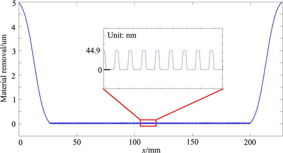
4.

Verification

In order to verify the simulation results and prove that the combination of the polishing parameter values listed in Table 6 is optimal, we conducted a verification test. Polishing parameter values were set as listed in Table 6. The experimental procedure and other conditions were the same as those described in Sec. 3.2.2. The test results are shown in Fig. 11. The PV of the residual error is 44.9 nm, which is smaller than any of the values listed in Table 5. Hence, it was verified that the method and simulation described above are appropriate and that the combination of the polishing parameter values shown in Table 6 is optimal for producing a surface with minimum residual error.

Fig. 11

Results of verification test.

5.

Conclusions

This paper reported that the residual error occurs because of the superposition of the TIF in the bonnet polishing process. Because the surface residual error is influenced by several parameters, experimental studies were conducted to study the effect of each parameter on the residual error. Practical bonnet polishing experiments are not appropriate for this purpose, because the residual error could be disturbed by conditions, such as initial surface profile error, instability of the TIF, and holding an error of the work-piece. Hence, orthogonal simulation experiments were designed for five major operating parameters at four levels: inner pressure, $z$ offset, raster distance, $H$-axis speed, and precession angle. It has been shown that the ranking of these parameters in terms of impact on the residual error, in decreasing order, is as follows: raster distance, $z$ offset, inner pressure, $H$-axis speed, and precession angle. Relatively small values for the raster distance and the inner pressure should be adopted together with a relatively large $z$ offset to reduce the residual error. We also determined and verified an optimal combination of five parameter values among these four levels based on the minimum residual error method.

The minimum residual error method proposed in this paper has been used to determine the optimal combination of five parameters for bonnet polishing when the tool radius is 80 mm. This method can also be effective for other sizes of tool radius.

Bonnet polishing technology is a subaperture polishing technology. A surface that is polished using other subaperture polishing technologies, such as IBF, MRF, and fluid jet polishing also has residual error. The minimum residual error method is also suitable for optimizing the polishing parameters of these processes.