Comprehensive numerical design approach for refractive laser beam shapers to generate annular irradiance profiles

Meijie Li; Youri Meuret; Fabian Duerr; Michael Vervaeke; Hugo Thienpont

doi:10.1117/1.OE.53.8.085103

6 August 2014 Comprehensive numerical design approach for refractive laser beam shapers to generate annular irradiance profiles

Meijie Li, Youri Meuret, Fabian Duerr, Michael Vervaeke, Hugo Thienpont

Author Affiliations +

Optical Engineering, Vol. 53, Issue 8, 085103 (August 2014). https://doi.org/10.1117/1.OE.53.8.085103

Abstract

A refractive laser beam shaper typically consists of either two plano-aspheric lenses or one thick lens with two aspherical surfaces. Ray mapping is a general optical design technique for irradiance reshaping based on geometric optics. Although ray mapping, in principle, allows generating any rotational-symmetric irradiance profile, in the literature this technique is mainly used to transform a Gaussian irradiance profile to a uniform rotational-symmetric profile. For more complex profiles, especially with low intensity in the inner region (such as annular profiles), a high sampling rate is required to ensure an accurate calculation of the surfaces. In practice, the high sampling rate increases the numerical effort to calculate the aspherical surfaces and the simulation time to verify the design considerably. In this work, we evaluate different sampling approaches and surface construction methods. This allows us to propose and demonstrate a comprehensive numerical approach to efficiently design refractive laser beam shapers to generate rotational-symmetric collimated beams with annular irradiance profiles. Ray tracing analysis for several annular irradiance profiles demonstrates the excellent performance of the designed lenses and the versatility of our design procedure.

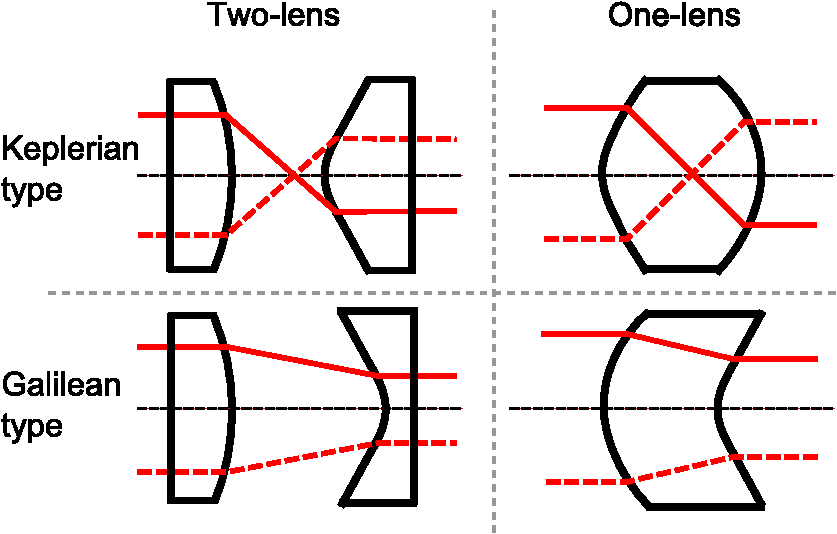
1. Introduction

Laser beam shaping is widely used in many industrial and medical applications. In most cases, a laser beam with a Gaussian irradiance profile is reshaped to have a uniform output profile, usually called a flat-top profile. In some applications, such as optical trapping,¹ atom guiding,² and laser additive manufacturing, an annular irradiance profile is required in order to ensure the optimal system performance. One example of such an annular irradiance profile is a dark hollow Gaussian (DHG) irradiance profile. There are various proposed techniques for laser beam shaping, especially to generate the rotational symmetric flat-top irradiance profiles. The simplest technique is either to truncate an expanded Gaussian beam³ or to use an apodized absorption filter.⁴ Such a technique allows one to generate uniform intensity patterns but is rather energy-inefficient. Typical energy-efficient approaches include refractive⁵ or reflective systems,⁶ diffractive elements,⁷ holograms,⁸ and microlens arrays.⁹ Among these techniques, refractive laser beam shapers are commonly used due to their high optical efficiency and simple structure.¹⁰

Four general configurations of refractive beam shapers are given in Fig. 1. They are formed either by two plano-aspheric lenses or by one single thick lens with two aspherical surfaces. The general optical design approach of such refractive beam shapers is based on ray mapping within the framework of geometric optics. The problem was initially proposed by Frieden in 1965.¹¹ Then, Kreuzer patented a design procedure in 1969¹² which is still widely used today. The ray mapping technique was further investigated and developed by Rhodes¹³ and Hoffnagle.⁵^,¹⁴^,¹⁵ Additional research led to the simplification of the practical design steps¹⁶ and optimization of the design algorithm for better performance.¹⁷

Fig. 1

Refractive laser beam shapers can be divided into four general configurations.

With the ray mapping technique, it is possible to generate any irradiance profile. However, published works mainly focus on flat-top profile generation and do not describe the practical steps of how to generate more complex profiles. For generating annular irradiance profiles with low intensity in the inner region, it is difficult to analytically derive a solution; the available numerical design approach¹⁶ to generate the elementary profiles does not work properly. Based on the ray mapping technique, this work presents an efficient numerical approach to design the refractive laser beam shapers to get annular irradiance profiles. With our design approach, both the numerical effort to calculate the aspherical surfaces and the simulation time to evaluate the designed lens system have been dramatically reduced. Also, the designed aspherical surfaces can be more accurately constructed by comparing different surface construction methods.

This article is structured as follows. In Sec. 2, the design procedure of how to design a refractive beam shaper is described. In the first design step for calculating the mapping function between the radial positions on the two aspherical surfaces, we have introduced both the conventional sampling method and our proposed alternative method. In the last step for constructing the designed surfaces, two methods are investigated and compared. One method is polynomial fitting and the other one is spline fitting which describes the surface profile by piecewise low degree polynomials. In Sec. 3, ray tracing results for different annular irradiance profiles are presented and analyzed. Taking a DHG profile as an example, the efficiency of two sampling methods is compared, highlighting the advantage of the alternative sampling method. Furthermore, the accuracy of two different surface construction methods is discussed and compared. In the end, additional simulation results for two other annular irradiance profiles are presented, underlining the versatility of our design procedure. Finally, in Sec. 4, conclusions are drawn and an outlook is given.

2. Design Procedure of Refractive Beam Shapers

The design of a refractive beam shaper based on geometric ray mapping is typically divided into four steps, which are listed in Table 1. Following these four design steps, this section describes both the conventional approach to transform a Gaussian irradiance profile to a flat-top profile¹⁶ and our alternative approach to generate annular profiles. The core differences between the two approaches for each step are also given in Table 1. Detailed explanations of different sampling methods and surface construction methods can be found later in their corresponding design steps. The two-lens Galilean-type configuration (see Fig. 2) is used for all designs in this article. It should be noticed that the presented approach can easily be adapted to design other configurations in Fig. 1 by only modifying the slope function Eq. (11) in Step 2.

Table 1

Design steps of refractive beam shapers.

Steps	Conventional approach: generating flat-top profiles	Our approach: generating annular profiles
Mapping $r$ to $R$	Sampling $P$	Sampling $R$
Calculating the surface slopes	Direct calculation	Same
Calculating the surface sags	Numerical integration of slopes	Same
Constructing the aspherical surfaces	Polynomial fitting with even exponents only	Spline fitting or polynomial fitting with even and odd exponents

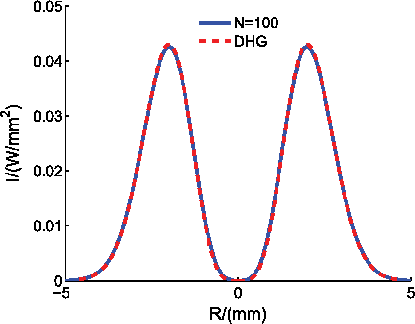
Fig. 2

Illustration of the two-lens Galilean-type configuration that transforms a collimated input beam to a collimated output beam: an arbitrary ray (from A to B) intersects the input plane at radius $r$ and arrives at the output plane at radius $R$ ; $z$ and $Z$ describe the sag values of the first and second aspherical surfaces; $t_{1}$ and $t_{2}$ define the thickness of the first and second aspherical surfaces; $D$ is the separation between the two lenses.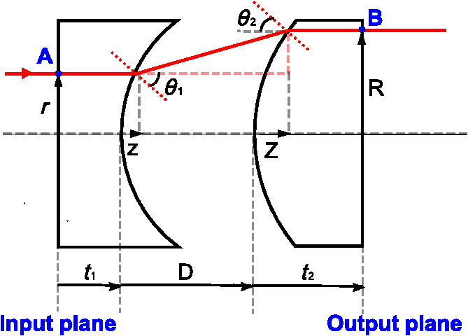

2.1.

Step 1: Mapping $r$ to $R$

Based on the law of conservation of energy, the power at the input plane is equal to the power at the output plane assuming there is no energy loss through the lens system. In order to map every radial coordinate $r$ to $R$ , the power inside each circle of the input radial coordinate $r$ should be the same as the power at the inside of each circle of the output radial coordinate $R$ .

Both the input and output irradiance profiles are rotationally symmetric, and can be described by functions $F_{in} (r)$ and $F_{out} (R)$ . The encircled power within $r$ at the input plane is a function of $r$ , given by the integral function $G_{in} (r)$ :

Eq. (1)

G_{in} (r) = 2 π \int_{0}^{r} F_{in} (x) \cdot x \cdot d x .

Similarly, at the output plane, the function $G_{out} (R)$ calculates the encircled power within $R$ as

Eq. (2)

G_{out} (R) = 2 π \int_{0}^{R} F_{out} (x) \cdot x \cdot d x .

There are two possible ways to calculate the mapping relationship between $r$ and $R$ from Eq. (1) and Eq. (2). Conventionally, the total power $P$ is directly sampled into equal power bins and, for each power bin, the corresponding radial positions on the first aspherical surface $r$ and on the second aspherical surface $R$ are calculated accordingly. We call this method “sampling $P$ .” For annular irradiance profiles, we have found that the numerical calculation effort can be considerably reduced by sampling the output radial coordinate $R$ with alternative equidistant points. More precisely, the complexity of the input and output irradiance profiles has to be properly compared and the radial coordinate at the plane with the more complex profile should be sampled. As the desired annular output profile (e.g., a DHG profile) has a null intensity in the inner region, it is considered to be more complex than the input Gaussian distribution. The output radial coordinate $R$ should be sampled. Therefore, we name this alternative sampling method as “sampling $R$ .”

2.1.1.

Sampling $P$

The sampling $P$ method is commonly used in the literature to generate a flat-top irradiance profile. Here, both the total input and output power are normalized to 1 or 100%. First, the maximum radii at the input and output planes $r_{\max}$ and $R_{\max}$ should be properly chosen, so that sufficient power $P_{\max}$ (e.g., 99.9%) can be transferred from the input to the output. Then, the total power $P_{\max}$ is sampled by equal bins. Supposing the sampling number is $N$ , the sampling index $i$ becomes ${1,2, \dots, N}$ . There are a total of ( $N - 1$ ) bins. For each bin, the encircled power is then given as

Eq. (3)

P_{i} = {0, \frac{99.9 %}{N - 1}, 2 \times \frac{99.9 %}{N - 1}, \dots, 99.9 %} .

For each power bin, the corresponding radii at the input plane and output plane $r_{i}$ and $R_{i}$ can be derived from the inverse functions of $G_{in} (r)$ and $G_{out} (R)$ :

Eq. (4)

r_{i} = G_{in}^{- 1} (P_{i}),

Eq. (5)

R_{i} = G_{out}^{- 1} (P_{i}) .

In this way, $r$ is mapped to $R$ and the generated data pairs ${r_{i}, R_{i}}$ are used for further calculation.

2.1.2.

Sampling $R$

In order to generate annular irradiance patterns, we propose an equidistant sampling of the output radial coordinate $R$ as an efficient alternative. In this case, we work as follows:

1. A maximum value for $R$ has to be chosen large enough to transmit sufficient power $P$ (e.g., $P_{\max} = 99.9 %$ ). The value $R_{\max}$ should be verified to ensure a feasible aperture size for the designed lens. $R_{\max}$ is calculated by
Eq. (6)
$R_{\max} = G_{out}^{- 1} (P_{\max})$
2. $R_{\max}$ is equidistantly sampled by a sufficient number of points $N$ . Similarly to previous calculations, the sampling index $i$ is ${1,2, \dots, N}$ . Then
Eq. (7)
$R_{i} = {0, \frac{R_{\max}}{N - 1}, 2 \times \frac{R_{\max}}{N - 1}, \dots, R_{\max}} .$
3. The encircled power within $R_{i}$ is calculated by
Eq. (8)
$P_{i} = G_{out} (R_{i}) .$
4. The corresponding $r_{i}$ at the input plane is calculated by
Eq. (9)
$r_{i} = G_{in}^{- 1} (P_{i}),$

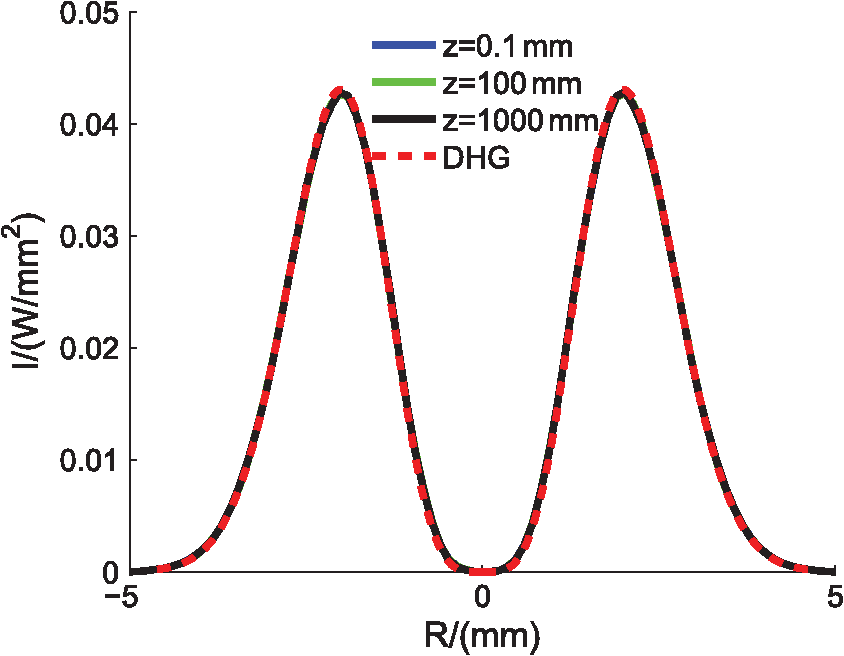
The calculated data pairs ${r_{i}, R_{i}}$ provide the mapping relationship between $r$ and $R$ .

2.2.

Step 2: Calculating the Surface Slopes

In Fig. 2, the slopes $v_{i}$ and $V_{i}$ are of two aspheric lens profiles which are defined as

Eq. (10)

v_{i} = \tan θ_{1}, V_{i} = \tan θ_{2} .

Due to the fact that both input and output beams are collimated, it follows from symmetry that the angles $θ_{1}$ and $θ_{2}$ are equal and as a result, $v_{i} = V_{i}$ .

By applying Snell’s law at each aspherical surface and keeping the optical path length between the input plane and the output plane constant, the slope values $v_{i}$ or $V_{i}$ can be described as a function of $r_{i}$ , $R_{i}$ , the separation between two lenses $D$ , and the refractive index of the lenses $n_{2}$ .¹² The local slope value at every radial position is calculated by

Eq. (11)

v_{i} = V_{i} = \frac{R_{i} - r_{i}}{\sqrt{(n_{2}^{2} - 1) {(R_{i} - r_{i})}^{2} + D^{2} {(n_{2} - 1)}^{2}}} .

2.3.

Step 3: Calculating the Surface Sags

After the calculation of the local slopes at each surface, the surface sags $z_{i}$ and $Z_{i}$ can be numerically calculated by integrating the slopes. The specific numerical integration method should be carefully selected in order to minimize the numerical calculation error. In this article, the trapezoidal numerical integration is used, available within MATLAB¹⁸ via the command “TRAPZ”.

2.4.

Step 4: Constructing the Aspherical Surfaces

In order to evaluate the optical performance of the beam shaper, it is necessary to construct smooth surfaces from the calculated discrete data sets of sag and slope values. We evaluate two different surface construction methods: polynomial fitting and spline fitting.

2.4.1.

Polynomial fitting

With polynomial fitting an analytical polynomial function is fitted to each set of sag points that describe each surface. To generate a flat-top profile, it is sufficient to use a polynomial function with only even exponents:¹⁶

Eq. (12)

z (r) = A_{1} r^{2} + A_{2} r^{4} + \dots + A_{n} r^{2 n} .

For more complex irradiance profiles such as annular profiles, we have found that a polynomial function with only even exponents is not adequate no matter how many coefficients are used. Instead, a polynomial function with both even and odd exponents should be used:

Eq. (13)

z (r) = A_{1} r + A_{2} r^{2} + \dots + A_{n} r^{n} .

Here, it should be noticed that $r$ is always positive and the pattern is rotationally symmetric.

The coefficients ${A_{1}, A_{2}, \dots, A_{n}}$ can be determined by either fitting the polynomial function $z (r)$ to the calculated sags or by fitting its first derivative $z^{'} (r)$ to the calculated slopes.¹⁶ In this article, the polynomial function is fitted to the calculated sags in MATLAB¹⁸ using the command “POLYFITN”. This algorithm calculates the coefficients of the polynomial function that fits the data set best by minimizing the least-squares.

2.4.2.

Spline fitting

As an alternative, spline fitting uses piecewise low order polynomial functions to match both calculated sag and slope values in order to describe the surface profile.¹⁹ We have used a continuous piecewise cubic spline to construct the designed aspherical surfaces in the optical ray tracing software ASAP²⁰ with the “SPLINE” command.

3. Ray Tracing Results and Discussions

Our designed refractive beam shapers are evaluated by ray tracing in ASAP and the simulation results are presented and discussed in this section.

The input and output irradiance profiles of our example to transform a Gaussian profile to a DHG profile are shown in Fig. 3. The input beam has a circular Gaussian irradiance profile. The irradiance of a Gaussian profile $I_{G}$ is expressed by

Eq. (14)

I_{G} (r) = I_{a} \times \exp [- 2 {(\frac{r}{w_{G}})}^{2}],

where

r

is the radial coordinate,

I_{a}

is the maximum (maximum) irradiance at

r = 0

, and

w_{G}

is the beam waist. The irradiance at the beam waist is equal to

I_{a} \times e^{- 2}

. In our example,

I_{a}

is calculated by normalizing the total power to 1, and

w_{G}

is 2.366 mm. The output beam has a DHG irradiance profile; therefore, the beam can be described by hollow Gaussian beams (HGBs).²¹ Then, the irradiance

I_{DHG}

is calculated by

Eq. (15)

I_{DHG} (r) = I_{b} \times {(\frac{r^{2}}{w_{DHG}^{2}})}^{2 n} \times \exp (- 2 \frac{r^{2}}{w_{DHG}^{2}}), n = 0,1, 2, \dots,

where

I_{b}

is a constant,

n

is the order of the HGB, and

r

is the radial coordinate. In the case where

n

is equal to 0, the DHG is identical by the fundamental Gaussian with beam waist

w_{DHG}

. As energy is conserved,

I_{b}

is calculated by also normalizing the total power to 1.

n

is chosen as 1 and

w_{DHG}

is 2 mm.

Fig. 3

Irradiance profiles: input Gaussian profile and output DHG profile. $r$ is the radial coordinate and $I$ is the irradiance.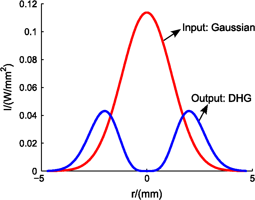

3.1.

Ray Tracing Results for Designs Obtained with Different Sampling Methods

Two sampling methods have been introduced in Step 1 of Sec. 2: sampling $P$ and sampling $R$ . In order to evaluate these two sampling methods, we have used both methods with different sampling numbers to design beam shapers that generate the same DHG profile. After constructing the calculated aspherical surfaces by spline fitting, both designs are simulated in ASAP and ray tracing results are compared.

With the sampling $P$ method, several beam shapers are designed to generate the DHG output profile by using different numbers of sampling points. For each design, a grid of $2001 \times 2001$ rays has been traced through the lens system with ASAP to directly generate the output intensity profile after the second lens. A comparison of the detected output profiles for different designs is given in Fig. 4. In order to match the required DHG profile, the number of sampling points $N$ has to be as large as 10,000. With fewer sampling points, the output profile departs from the expected DHG profile, especially for the center part. The reason for this is that the original sampling of equidistant power bins in combination with a null/very low intensity at the optical axis results in an equally low sampling rate of the second aspherical lens surface in that region. Therefore, a much higher overall sampling rate (thousands of bins) is necessary to achieve a sufficiently high sampling of the second aspherical lens surface close to the optical axis. This problem is solved by our proposed sampling $R$ method, as it samples the second aspherical surface with equidistant sampling points.

Fig. 4

Ray tracing results for designs obtained with sampling $P$ method for different number $N$ of sampling points: the shown simulation results (solid lines) in comparison with the required DHG profile (dashed line) reveal the high sampling rate that is necessary to achieve good agreement of the intensities especially in the central region.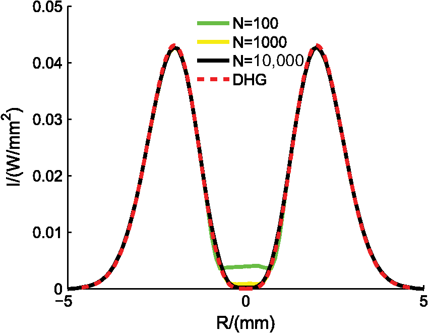

The ray tracing result for a design with sampling $R$ by only 100 sampling points is shown in Fig. 5. It clearly shows that 100 sampling points are already sufficient, which is much less than when we sample the encircled power $P$ . With fewer sampling points, the numerical efforts to calculate the lens profiles and the simulation time to evaluate the designed beam shaper can be drastically reduced, as we will explain in more detail in the next section. This finding highlights the benefits of the sampling $R$ method to efficiently generate annular irradiance profiles.

Fig. 5

Ray tracing results for designs obtained with sampling $R$ method for a moderate number of only 100 sampling points: the simulated DHG irradiance profile (solid line) matches the required DHG output profile (dashed line) very well.

3.2.

Ray Tracing Results for Designs Obtained with Different Surface Construction Methods

We consider two possible ways to construct the surfaces from the calculated surface sages and/or slopes: polynomial fitting and spline fitting. Designs obtained with these two methods are simulated in ASAP. For each simulation, a grid of $2001 \times 2001$ rays is traced and evaluated not only at the plane directly after the second lens, but also at planes with certain distances from the second lens along the $z$ axis. In this way, it is possible to verify how well the generated output profile is maintained after propagation, which is a good indication of the collimation quality of the output beam.

For the method of polynomial fitting, a polynomial function in Eq. (13) with 21 coefficients is used. Ray tracing results for the design with a polynomial fitting are presented in Fig. 6. The dashed line is the required DHG profile, whereas the different solid lines correspond to the simulation results for the output profile after certain propagation distances along the $z$ axis. For $z = 0.1 mm$ , the output profile corresponds well to the expected DHG profile. The irradiance profile starts to deviate from the DHG profile when it propagates over distances beyond 100 mm, and after 1000 mm, the difference is very clear. For the design of transforming a Gaussian irradiance profile to a DHG profile, a recently published article has proposed that the first aspherical surface should be described by a polynomial function with fractional instead of integer exponents.²² This proposed polynomial function with fractional exponents has provided a very low mapping error, yet the generated DHG profile seems to not be maintained well enough after propagating by 1000 mm.

Fig. 6

Ray tracing results for designs obtained with polynomial fitting: $z$ is the propagation distance from the beam shaper. After propagating only 0.1 mm, the simulated output irradiance profile still fits well with the required DHG profile (dashed line); however, the irradiance profile begins to deviate from the required DHG profile with increased propagation distances.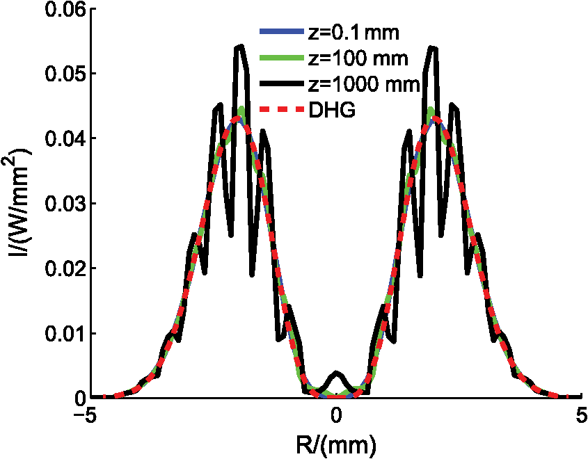

Figure 7 shows the simulation results for the design obtained with spline fitting. In this case, the irradiance profile agrees well with the required DHG profile over the complete propagation trajectory, which proves perfect collimation of the output beam. It should be noticed that the simulation time for surfaces constructed by spline fitting is strongly dependent on the number of piecewise polynomial functions, which is defined by the number sampling points. Fewer sampling points significantly reduce the simulation time.

Fig. 7

Ray tracing results for designs obtained with spline fitting: $z$ is the propagation distance from the beam shaper. The simulated irradiance profiles (solid lines) are in excellent agreement with the required DHG profile (dashed line) over the complete propagation trajectory.

3.3.

Further Examples of Generated Annular Irradiance Profiles

The presented design approach allows the design of refractive laser beam shapers for various complex irradiance profiles, which are rotational symmetric. As a further example for annular profiles, a Gaussian beam is transformed into an output beam with a cosine irradiance profile, which has both a center peak and an outside ring. The output cosine irradiance profile is a cosine function where a constant is added so that the minimum irradiance is 0. Similarly, we used 100 points to sample the output radial coordinate $R$ and spline fitting for the surface construction. The ray tracing result with a grid of $2001 \times 2001$ rays is given in Fig. 8. The simulation result is in good agreement with the expected cosine profile.

Fig. 8

The output cosine irradiance profile is a cosine function shifted upward, so that the minimum irradiance is 0. The simulation result (solid line) of the designed beam shaper to transform a Gaussian profile to a cosine profile shows good agreement with the expected output profile (dashed line).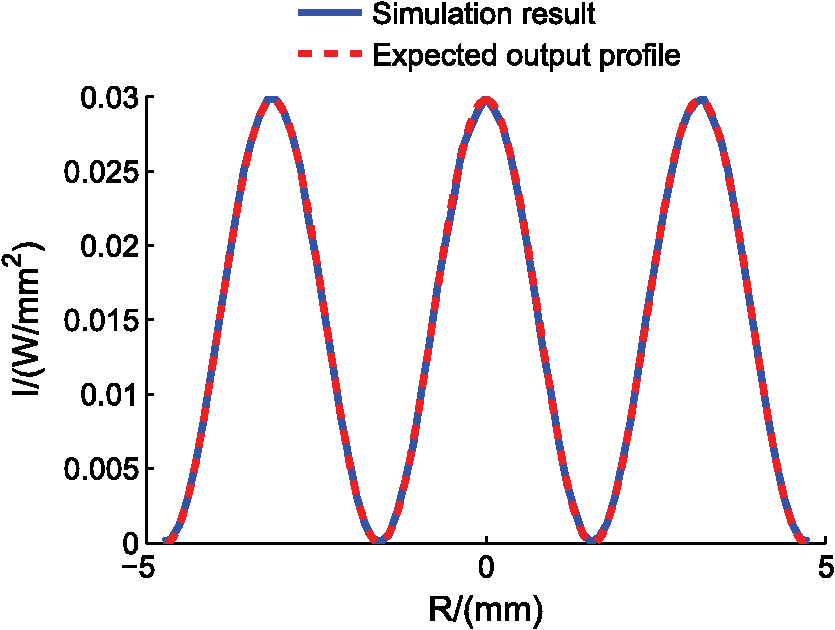

As another example, the laser beam shaper is designed to generate a sine irradiance output profile which has two concentric rings. The output sine irradiance profile is a sine function shifted upward to have zero minimum irradiance and moved rightward to have a rotational symmetry axis at 0. Applying the same design approach and simulation procedure, the ray tracing result is shown in Fig. 9. It also agrees well with the expected sine profile.

Fig. 9

The output sine irradiance profile is a sine function shifted upward to have zero minimum irradiance and moved rightward to have a rotational symmetry axis at 0. The simulation result (solid line) of the designed beam shaper to transform a Gaussian profile to a sine profile shows good agreement with the expected output profile (dashed line).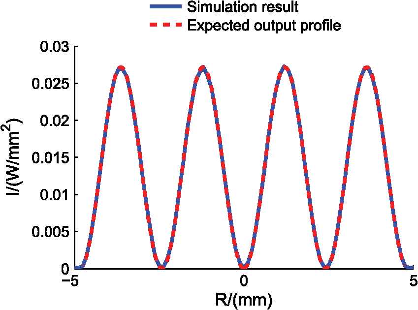

These two examples conform the versatility of our design procedure and highlight its potential use for generating different annular irradiance profiles with single or multiple rings.

4. Conclusion

Ray mapping-based optical design is a powerful technique to design the refractive laser beam shapers for irradiance redistribution. If the desired profile is more complex than a flat-top profile, especially with low intensity in the inner region such as annular profiles, the available design procedures have to be modified. In the first step to calculate the mapping function, we have identified an alternative efficient sampling method. Our method by sampling the output radial coordinate $R$ requires much fewer sampling points than the conventional sampling method by sampling the encircled power $P$ . Normally, only 100 sampling points are sufficient. Depending on the particular beam shaping problem, the optical designer should carefully identify and select the appropriate sampling method that allows an accurate and fast design and reconstruction of the lens surfaces. In the last step, to construct the calculated aspherical surfaces, both polynomial and spline fittings can provide satisfactory results. For a polynomial fitting, the polynomial series should have both even and odd exponents rather than only even exponents. Compared with the polynomial fitting, spline fitting has better precision because the generated annular profile can propagate unchanged though a much longer distance along the optical axis.

The described design approach in this article can be easily followed to design a refractive lens system that transforms a Gaussian irradiance pattern to an annular pattern with rotational symmetry. It should be noticed that both input and output beams are collimated, and are thus described by plane wave fronts. A generalization to cope with arbitrary wave fronts will be addressed in future work.

Acknowledgments

The work reported in this article is mainly funded by a SBO Project Grant No. 110070: eSHM with AM of the Agency for Innovation by Science and Technology (IWT). It is also supported by the Research Foundation, Flanders (FWO-Vlaanderen) that provides a postdoctoral grant to Fabian Duerr, and in part by the IAPBELSPO grant IAP P7-35 photonics@be, the Industrial Research Funding (IOF), FWO (G008413N), the MP1205, COST Action, the Methusalem and Hercules foundations and the OZR of the Vrije Universiteit Brussel (VUB).

References

1.

T. Kugaet al., “Novel optical trap of atoms with a doughnut beam,” Phys. Rev. Lett., 78 (25), 4713 –4716 (1997). http://dx.doi.org/10.1103/PhysRevLett.78.4713 PRLTAO 0031-9007 Google Scholar

2.

J. YinY. Zhu, “Optical potential for atom guidance in a dark hollow laser beam,” J. Opt. Soc. Am. B, 15 (1), 25 –33 (1998). http://dx.doi.org/10.1364/JOSAB.15.000025 JOBPDE 0740-3224 Google Scholar

3.

J. P. CampbellL. G. Deshazer, “Near fields of truncated-Gaussian apertures,” J. Opt. Soc. Am., 59 (11), 1427 –1429 (1969). http://dx.doi.org/10.1364/JOSA.59.001427 JOSAAH 0030-3941 Google Scholar

4.

S. P. Changet al., “Transformation of Gaussian to coherent uniform beams by inverse-Gaussian transmittive filters,” Appl. Opt., 37 (4), 747 –752 (1998). http://dx.doi.org/10.1364/AO.37.000747 APOPAI 0003-6935 Google Scholar

5.

J. A. HoffnagleC. M. Jefferson, “Design and performance of a refractive optical system that converts a Gaussian to a flattop beam,” Appl. Opt., 39 (30), 5488 –5499 (2000). http://dx.doi.org/10.1364/AO.39.005488 APOPAI 0003-6935 Google Scholar

6.

V. Oliker, “Optical design of freeform two-mirror beam-shaping systems,” J. Opt. Soc. Am. A, 24 (12), 3741 –3752 (2007). http://dx.doi.org/10.1364/JOSAA.24.003741 JOAOD6 0740-3232 Google Scholar

7.

D. PalimaJ. Glückstad, “Gaussian to uniform intensity shaper based on generalized phase contrast,” Opt. Express, 16 (3), 1507 –1516 (2008). http://dx.doi.org/10.1364/OE.16.001507 OPEXFF 1094-4087 Google Scholar

8.

T. DreselM. BeyerleinJ. Schwider, “Design and fabrication of computer-generated beam-shaping holograms,” Appl. Opt., 35 (23), 4615 –4621 (1996). http://dx.doi.org/10.1364/AO.35.004615 APOPAI 0003-6935 Google Scholar

9.

F. Wippermannet al., “Beam homogenizers based on chirped microlens arrays,” Opt. Express, 15 (10), 6218 –6231 (2007). http://dx.doi.org/10.1364/OE.15.006218 OPEXFF 1094-4087 Google Scholar

10.

L. A. RomeroF. M. Dickey, “Lossless laser beam shaping,” J. Opt. Soc. Am. A, 13 (4), 751 –760 (1996). http://dx.doi.org/10.1364/JOSAA.13.000751 JOAOD6 0740-3232 Google Scholar

11.

B. R. Frieden, “Lossless conversion of a plane laser wave to a plane wave of uniform irradiance,” Appl. Opt., 4 (11), 1400 –1403 (1965). http://dx.doi.org/10.1364/AO.4.001400 APOPAI 0003-6935 Google Scholar

12.

J. L. Kreuzer, “Coherent light optical system yielding an output beam of desired intensity distribution at a desired equiphase surface,” (1969). Google Scholar

13.

P. W. RhodesD. L. Shealy, “Refractive optical systems for irradiance redistribution of collimated radiation their design and analysis,” Appl. Opt., 19 (20), 3545 –3553 (1980). http://dx.doi.org/10.1364/AO.19.003545 APOPAI 0003-6935 Google Scholar

14.

J. A. HoffnagleC. M. Jefferson, “Refractive optical system that converts a laser beam to a collimated flat-top beam,” (2001). Google Scholar

15.

J. A. HoffnagleC. M. Jefferson, “Beam shaping with a plano-aspheric lens pair,” Opt. Eng., 42 (11), 3090 –3099 (2003). http://dx.doi.org/10.1117/1.1613957 OPEGAR 0091-3286 Google Scholar

16.

J. A. McNeil, “Design of laser beam shaping optics—a simple algebraic method,” Proc. SPIE, 6872 68720D (2008). http://dx.doi.org/10.1117/12.763626 PSISDG 0277-786X Google Scholar

17.

H. Maet al., “Improvement of Galilean refractive beam shaping system for accurately generating near-diffraction-limited flattop beam with arbitrary beam size,” Opt. Express, 19 (14), 13105 –13117 (2011). http://dx.doi.org/10.1364/OE.19.013105 OPEXFF 1094-4087 Google Scholar

18.

Software MATLAB, (2014) http://www.mathworks.com/ January ). 2014). Google Scholar

19.

C. de Boor, A Practical Guide to Splines, Springer-Verlag, New York (1978). Google Scholar

20.

Software ASAP, (2014) http://www.breault.com/software/asap.php/ January ). 2014). Google Scholar

21.

Y. CaiQ. Lin, “Hollow elliptical gaussian beam and its propagation through aligned and misaligned paraxial optical systems,” J. Opt. Soc. Am. A, 21 (6), 1058 –1065 (2004). http://dx.doi.org/10.1364/JOSAA.21.001058 JOAOD6 0740-3232 Google Scholar

22.

F. DuerrH. Thienpont, “Refractive laser beam shaping by means of a functional differential equation based design approach,” Opt. Express, 22 (7), 8001 –8011 (2014). http://dx.doi.org/10.1364/OE.22.008001 OPEXFF 1094-4087 Google Scholar

Biography

Meijie Li received her BS degree in electronics science and technology from Shandong University, China, in 2008. She graduated from Erasmus Mundus Master program “OpSciTech” in 2010 with a double MS degree: one from Warsaw University of Technology (WUT), Poland, and the other one from Delft University of Technology (TUD), the Netherlands. She is now a PhD student at Vrije Universiteit Brussel (VUB), Belgium, in optical design and simulation. She is a student member of SPIE.

Youri Meuret graduated in physics in 1998 and received his PhD degree in applied sciences in 2003, both at Ghent University, Belgium. Afterward he was responsible for a research group on novel projection displays and illumination systems at Department of Applied Physics and Photonics, Vrije Universiteit Brussel (VUB). Since 2013 he is associate professor at the Light and Lighting Laboratory, KU Leuven, Belgium.

Fabian Duerr graduated in physics from the Karlsruhe Institute of Technology (KIT), Germany in 2008. He then joined the Department of Applied Physics and Photonics at the Vrije Universiteit Brussel (VUB), Belgium in 2009, where he received his PhD degree in applied sciences in 2013. As a postdoctoral research fellow of FWO-Vlaanderen, currently he is responsible for a research group that explores the potential of novel free-form optical designs. He is a member of SPIE and OSA.

Michael Vervaeke received his PhD degree in electrotechnical engineering on photonic modeling and packaging of chip-level interconnects. He is now responsible for the ultraprecision fabrication technologies for polymer optics and photonic systems at the Brussels Photonics Team. He authored more than 56 publications in international conference proceedings in his research field as well as in education, and authored or co-authored more than 11 journal publications.

Hugo Thienpont graduated as an electrotechnical engineer in 1984 and received his PhD degree in applied sciences in 1990, both at the Vrije Universiteit Brussel (VUB), Belgium. He became a professor at the Faculty of Engineering in 1994. He is now the managing director of Brussels Photonics Team (BPHOT). He is a fellow member of SPIE and EOS, and a member of OSA and the IEEE Photonics Society.

CC BY: © The Authors. Published by SPIE under a Creative Commons Attribution 4.0 Unported License. Distribution or reproduction of this work in whole or in part requires full attribution of the original publication, including its DOI.

Citation Download Citation

Meijie Li, Youri Meuret, Fabian Duerr, Michael Vervaeke, and Hugo Thienpont "Comprehensive numerical design approach for refractive laser beam shapers to generate annular irradiance profiles," Optical Engineering 53(8), 085103 (6 August 2014). https://doi.org/10.1117/1.OE.53.8.085103

Published: 6 August 2014

Access the abstract

JOURNAL ARTICLE
7 PAGES

DOWNLOAD PAPER SAVE TO MY LIBRARY

GET CITATION

CITATIONS

Cited by 6 scholarly publications.

Explore citations on Lens.org

KEYWORDS

Ray tracing

Beam shaping

Collimation

Computer simulations

Lens design

Lenses

Optical simulations

1.

Introduction