Relating the statistics of the angle of linear polarization to measurement uncertainty of the Stokes vector

Meredith Kupinski; Russell Chipman; Eric Clarkson

doi:10.1117/1.OE.53.11.113108

12 November 2014 Relating the statistics of the angle of linear polarization to measurement uncertainty of the Stokes vector

Meredith Kupinski, Russell Chipman, Eric Clarkson

Author Affiliations +

Optical Engineering, Vol. 53, Issue 11, 113108 (November 2014). https://doi.org/10.1117/1.OE.53.11.113108

Abstract

This work shows an analytic solution to the central moments of the angle of linear polarization (AoLP) when the linear Stokes parameters are independent and Gaussian distributed with different means but equal variance. Such a result is useful for distinguishing AoLP features from noise in polarimetry. When the DoLP is high relative to the measurement uncertainty of the linear Stokes vector, AoLP statistics have been shown to be well approximated by a Gaussian distribution. When the DoLP is zero, AoLP values are uniformly distributed. In general, the probability density function (PDF) of AoLP does not have a closed-form solution and this is the first report, to our knowledge, on an exact analytic form for the central moments of the AoLP. This analytic form will be useful when the AoLP is of interest even when the DoLP is low and the corresponding PDF on the AoLP is in between the extreme cases of a Gaussian or a uniform distribution. We also show that a simple propagation of error (PE) analysis underestimates the AoLP variance at extremely low DoLP but is verified for cases of DoLP that are high relative to the Stokes measurement uncertainty. An example use of the AoLP variance in imaging polarimetry is presented.

1. Introduction

The Stokes vector that is limited to the three first components is commonly referred to as the linear Stokes vector¹ and includes intensity and two linear Stokes parameters. From its measurement, two primary parameters of interest are calculated: the degree of linear polarization (DoLP) and the angle of linear polarization (AoLP). The AoLP and DoLP are nonlinear transforms of the two linear Stokes parameters from Cartesian to polar coordinates. The AoLP expresses the orientation of the linear polarization state. The DoLP expresses the magnitude of the linear polarization state. This work presents an exact analytic solution for the central moments of the AoLP when the linear Stokes parameters are drawn from uncorrelated Gaussian distributions of different means but equal variance. Fluctuations due to a change in the object’s polarization state during data acquisition (e.g., atmospheric turbulence) or fluctuations due to system artifacts (e.g., error from mechanical motion of optical components) could potentially introduce significant correlations. To test the validity of the uncorrelated assumption both the polarimetric instrumentation and the postprocessing calculations must be considered. If in postprocessing, different raw measurements are used to calculate each linear Stokes parameter then the measurement statistics will be uncorrelated owing to the independence of each measurement. Correlations would be introduced by reusing an individual measurement in the calculation of both linear Stokes parameters. Division of amplitude, aperture, or wavefront polarimeters traditionally use independent measurements to estimate each linear Stokes parameter. Traditional wire-grid polarizers also produce linear Stokes parameters with measurement noise that is uncorrelated since a different pair of independent measurements are used to calculate each.

If the Stokes parameters are calculated by combining a weighted sum of numerous independent measurements then, owing to the central limit theorem, a Gaussian probability density function (PDF) is expected with increasing confidence as the number of measurements used in the calculation increases.² For example, modulated polarimeters collect a series of measurements while simultaneously changing the instrument’s polarimetric response. Using this strategy, the object’s polarization can be encoded temporally, spatially, and/or spectrally in the measurements. Then, in postprocessing numerous independent measurements are combined, usually by fitting to a model, to form an estimate of the object’s polarization.

Physical models of polarization are often specified in polar coordinates (e.g., astronomy and material scattering properties), therefore, characterizing AoLP statistics is of interest.³^,⁴ Although an integral form of the PDF of the AoLP is known, this is the first report, to our knowledge, on an exact analytic expression for the central moments of the AoLP and their relation to the measurement uncertainty of the linear Stokes vector. When the DoLP is high relative to the measurement uncertainty of the linear Stokes vector, AoLP statistics have been shown to be well approximated by a Gaussian distribution;⁵ this is consistent with the results presented in this paper. As the DoLP approaches the measurement uncertainty of the linear Stoke parameters, the distribution on AoLP is no longer well approximated by a Gaussian distribution; this is also consistent with the results presented in this paper. This low DoLP limit is of interest and importance to researchers in astrophysics,⁵ reconnaissance,⁶ and atmospheric aerosol retrieval.⁷

2. Mathematical Results

Consider the two linear Stokes parameters $q$ and $u$ as independent and normally distributed random variables with equal variance, $pr (q) = N (\bar{q}, σ_{u, q}^{2})$ and $pr (u) = N (\bar{u}, σ_{u, q}^{2})$ . Here, all quantities are normalized by the intensity (i.e., the first linear Stokes component), as in $q = Q / I$ and $u = U / I$ where $I$ denotes the intensity. In practice, the PDF on $q$ and $u$ will depend upon how these quantities are measured. If in postprocessing the Stokes parameters are calculated from a sum, or weighted sum, of raw measurements then we can argue from the central limit theorem that the $pr (u)$ and $pr (u)$ will be approximately Gaussian if the raw measurements are sufficiently independent. From $pr (u)$ and $pr (u)$ , a transformation of random variables is used to obtain $pr (θ)$ as a function of the means and variance of the two linear Stokes parameters. Beginning with the joint PDF

Eq. (1)

{pr}_{θ, d} (θ, d) = {pr}_{q, u} [d \cos (2 θ), d \sin (2 θ)] | \det [\begin{matrix} \cos (2 θ) & 2 d \sin (2 θ) \\ \sin (2 θ) & - 2 d \cos (2 θ) \end{matrix}] | = \frac{2 d}{2 π σ_{u, q}^{2}} \exp {- \frac{{[d \cos (2 θ) - \bar{q}]}^{2} + {[d \sin (2 θ) - \bar{u}]}^{2}}{2 σ_{u, q}^{2}}},

where

θ

is the AoLP and

d

is the DoLP. Here, the transformations

q = d \cos (2 θ)

and

u = d \sin (2 θ)

have been used to relate the linear Stokes parameters to the AoLP and the DoLP. Marginalizing over AoLP yields the Rice distribution on DoLP.⁸ Marginalizing over the DoLP to obtain the PDF of AoLP

Eq. (2)

pr (θ) = \int_{0}^{1} d p {pr}_{θ, d} (θ, p) = \frac{1}{π} e^{\frac{- {\bar{d}}^{2}}{2}} \int_{0}^{\infty} d \tilde{p} \tilde{p} e^{\frac{- {\tilde{p}}^{2}}{2}} e^{\tilde{p} [\bar{q} \cos (2 θ) + \bar{u} \sin (2 θ)]},

where all parameters denoted with the tilde have been normalized by

σ_{u, q}

, e.g.,

\tilde{\bar{u}} = (\bar{u} / σ_{u, q})

and

{\tilde{\bar{d}}}^{2} = {\tilde{\bar{u}}}^{2} + {\tilde{\bar{q}}}^{2}

. This integral form is the moment generating function of the Rayleigh distribution; it is not closed-form but can be expressed using error functions as in Ref. 9.

The definition of the $α$ -order central moment of the AoLP is

Eq. (3)

〈 {(θ - \bar{ϕ})}^{α} 〉 = \int_{\bar{ϕ} - π / 2}^{\bar{ϕ} + π / 2} d θ pr (θ) {(θ - \bar{ϕ})}^{α} .

Here,

\bar{ϕ} = 1 / 2 atan

(

\bar{u} / \bar{q}

) is half the angle between the mean of

{pr}_{q, u} (q, u)

and the

q

-axis, as depicted in Fig. 1. The distribution

pr (θ)

is symmetric about

\bar{ϕ}

and the expectation over all possible values of

θ

is evaluated over a

π

interval centered on

\bar{ϕ}

. This definition of

pr (θ)

avoids the spurious values in calculations of angular quantities if wrapping of the directional statistics is not accounted for.

Fig. 1

In (a) and (b), the yellow points are samples from ${pr}_{q, u} (q, u)$ where the spread of this distribution is characterized by $\tilde{\bar{d}} = \sqrt{{\bar{u}}^{2} + {\bar{q}}^{2}} / σ_{u, q}$ and both low and high examples of this value are provided. Two points are labeled: the mean $\tilde{\bar{r}}$ and the $n$ ’th sample ${\tilde{r}}_{n}$ . $\bar{ϕ}$ is the angle of linear polarization (AoLP) of $\tilde{\bar{r}}$ and $θ_{n}$ is the AoLP of ${\tilde{r}}_{n}$ . The AoLP’s central moments are related to the angular spread from $\bar{ϕ}$ . A histogram of ( $θ - \bar{ϕ}$ ) is given in (c) and (d); the red line is a least-squares fit to a Gaussian distribution.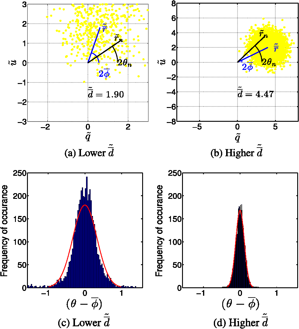

In the Appendix, we show that the $α$ -order central moment of the AoLP can be equivalently expressed as

Eq. (4)

〈 {(θ - \bar{ϕ})}^{α} 〉 = \frac{1}{2^{α + 1} π} \sum_{n = - \infty}^{\infty} B_{n}^{α} f_{n} (\tilde{\bar{d}}),

where the scalar

B_{n}^{α}

and the function

f_{n}

are defined below. As expected, the central moments are circularly symmetric with respect to the average value of the AoLP, in other words, only the DoLP and the uncertainty of the linear Stokes parameters

σ_{u, q}

are in this expression;

\bar{ϕ}

is not. The term that can be factored as independent of the DoLP and only dependent upon the order of the moment is

Eq. (5)

B_{n}^{α} = \frac{1}{2 π} \int_{- π}^{π} β^{α} e^{- in β} d β,

where

β = 2 θ - 2 \bar{ϕ}

describes the angular deviation as depicted in Fig. 1. For the first and second moments, which are calculated in Secs. 3 and 4

Eq. (6)

B_{n}^{1} = {\begin{cases} \frac{{(- 1)}^{n} i}{n} & \forall n \neq 0 \\ 0 & otherwise \end{cases},

Eq. (7)

B_{n}^{2} = {\begin{cases} \frac{2 {(- 1)}^{n}}{n^{2}} & \forall n \neq 0.1 c m \\ \frac{π^{2}}{3} & otherwise . \end{cases}

The other term depends on the DoLP and the linear Stokes uncertainty, but not the

α

moment

Eq. (8)

f_{n} (\tilde{\bar{d}}) = {\begin{cases} \sqrt{\frac{π^{3}}{2}} e^{\frac{- {\bar{d}}^{2}}{4}} \bar{d} [I_{\frac{n - 1}{2}} (\frac{{\bar{d}}^{2}}{4}) + I_{\frac{n + 1}{2}} (\frac{{\bar{d}}^{2}}{4})] & \forall n \neq 0 \\ 2 π & otherwise . \end{cases}

Here,

I

is a modified Bessel function of the first kind. Appendix contains a detailed derivation of Eq. (4) from Eq. (3).

The analytic expression for the AoLP central moments is an infinite sum which, in practice, must be truncated, therefore, the computed value depends upon the number of terms retained

Eq. (9)

〈 {(θ - \bar{ϕ})}^{α} 〉 \approx 〈 \hat{{(θ - \bar{ϕ})}^{α}} 〉 (K) = \frac{1}{2^{α + 1} π} \sum_{n = - K}^{K} B_{n}^{α} f_{n} (\tilde{\bar{d}}) .

When performing this computation, it is useful to notice that

f_{- n} = f_{n}

. The analytic form for the square root of the second central moment, i.e., the standard deviation, of the AoLP is shown in Fig. 2(b) for

K = 500

.

Fig. 2

The AoLP standard deviation is reported in degrees and calculated from (a) sample statistics [Eq. (12)], (b) the new analytic form presented in this work [Eq. (9)], and (c) the propagation of error approximation [Eq. (11)]. The maximum differences between methods (b) and (c) with respect to method (a) are 0.03 deg and 4.72 deg, respectively. This agreement between an asymptotically unbiased estimate and the analytic form is expected and verifies the precision of the analytic expression and its derivation presented in the Appendix.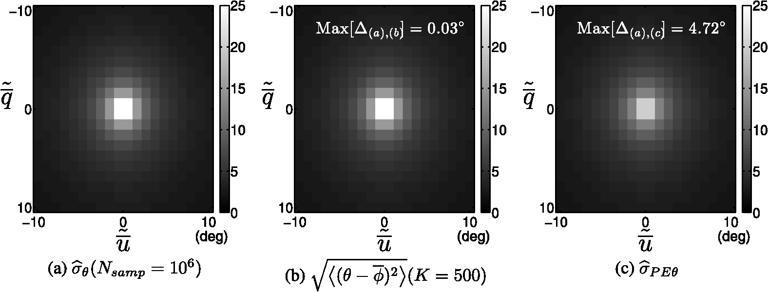

3. Computational Results

To verify the precision of the new analytic expression for the central moments of the AoLP, the square root of the second central moment (i.e., $α = 2$ ) is compared to two other numerical methods for calculating the AoLP standard deviation.

When a random variable of unknown variance has a nonlinear relationship to random variables of known variance the propagation of error (PE) method approximates the unknown variance by a truncated Taylor series as described in Ref. 10. When the linear Stokes parameters are uncorrelated, the PE approximation of the AoLP variance is

Eq. (10)

σ_{θ}^{2} \approx σ_{u}^{2} {(\frac{\partial θ}{\partial u})}^{2} + σ_{q}^{2} {(\frac{\partial θ}{\partial q})}^{2} .

By applying the assumption of equal variances for each linear Stokes parameter, the PE approximation becomes

Eq. (11)

{\hat{σ}}_{PE θ} = \frac{1}{2 \tilde{d}} = \frac{σ_{u, q}}{2 d},

which is displayed in Fig. 2(c).

The AoLP variance can also be calculated directly from $N_{samp}$ linear Stokes parameter samples

Eq. (12)

{\hat{σ}}_{θ}^{2} (N_{samp}) = \frac{1}{N_{samp}} \sum_{n = 1}^{N_{samp}} {‖ (θ_{n} - \bar{ϕ}) ‖}^{2} = \frac{1}{N_{samp}} \sum_{n = 1}^{N_{samp}} {[\frac{1}{2} acos (\frac{\bar{r} \cdot r_{n}}{| \bar{r} | | r_{n} |})]}^{2},

where

r_{n}

is the

n

’th sample generated by sampling from the Gaussian distributions

pr (q)

and

pr (u)

, the mean values of these distributions are

\bar{r} = [\bar{u}, \bar{q}]

, and the dot product

\bar{r} \cdot r_{n}

is used to calculate half of the angle between the vectors (

θ_{n} - \bar{ϕ}

) (depicted in Fig. 1). This sample variance is asymptotically unbiased, therefore, it will approach the true value of the AoLP variance as

N_{samp}

increases. To verify the precision of the analytic form, a true value for the AoLP variance is needed. To provide this comparison, the sample variance is calculated using a very large number of samples. The calculation using

N_{samp} = 10^{6}

is displayed in Fig. 2(a). The analytic form is closer to the sample variance than the PE approximation; the maximum difference is given as a text box in Fig. 2 and is 0.03 deg for the analytic form and 4.72 deg for the PE approximation.

To investigate the sensitivity between number of terms retained in Eq. (9) and the AoLP variance, a comparison is shown in Fig. 3(a). The number of terms required for convergence depends upon the AoLP variance. Accuracy at low AoLP variances (i.e., high DoLP) requires retaining more terms. For low DoLP environments and $σ_{θ} > 10 \deg$ , convergence is achieved at even 20 terms. This convergence behavior is advantageous since the analytic expression for AoLP variance is most useful in low DoLP environments. In relatively high DoLP environments, the analytic expression is not necessary because simpler approximations for the variance of AoLP, such as the PE method, are valid.

Fig. 3

(a) To show the effect of truncating the infinite sum in Eq. (4), the calculation is compared for different numbers of terms retained. Convergence with respect to $K$ is slowest at low values of $σ_{θ}$ . The results become indistinguishable between $K = 250$ and $K = 500$ . The black line is ${\hat{σ}}_{PE θ}$ and does not agree with the sample statistics or the analytic form at high values of $σ_{θ}$ . (b) The under estimation of $σ_{θ}$ by ${\hat{σ}}_{PE θ}$ is shown to occur at DoLP values below 2% when 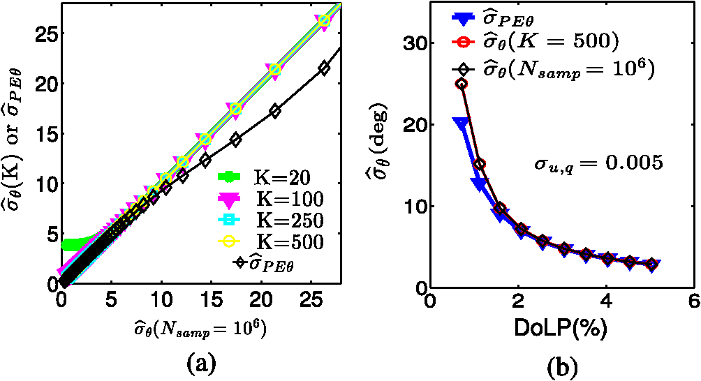$σ_{u, q} = 0.005$ .

Figure 3(b) is a comparison between the PE estimate and the analytic expression for the AoLP variance at low DoLP. For $σ_{u, q} = 0.005$ , the two methods agree above about 2% DoLP. For DoLP lower than 2%, the methods begin to disagree and the PE analysis predicts lower values for $σ_{θ}$ . At 1% DoLP, the difference between the two methods is approximately 5 deg. This difference is potentially significant because statistical testing becomes most useful when the DoLP is low.

4. Example Application in Imaging Polarimetry

Figure 4 shows a cloud measurement from the Ground-based Multiangle SpectroPolarimetric Imager (GroundMSPI).¹¹ This is an ideal application for our analytic AoLP variance since 47% of the pixels in the scene are at or below 2% DoLP; see Fig. 4(b). AoLP statistical analysis can be used to test GroundMSPI’s sensitivity in distinguishing single from multiple scattering events. In the case of single scattering, the AoLP of the cloud will either be the same as the AoLP of the sky or 90 deg from it as described in Refs. 12 and 13. Given GroundMSPI’s measurement uncertainty in the Stokes parameters of $\pm 0.005$ ,¹⁴ the analytic form presented in this paper is used to calculate the standard deviation of the AoLP measured at each image pixel. Pixels are selected from the GroundMSPI image based on three different $σ_{AoLP}$ thresholds of: 3 deg, 6 deg, and 9 deg. These thresholds result in including 40%, 48%, and 60% of the image pixels; respectively. In Fig. 5, these AoLP values are plotted versus DoLP to separate sky from cloud pixels. The AoLP is plotted with error bars $\pm 2 σ_{θ}$ from the measured value. The $\pm 2 σ_{θ}$ interval has been shown in Ref. 5 to produce a 95.45% confidence level on AoLP. The AoLP uncertainty is lowest for the sky measurements since these have a higher DoLP value than the cloud [see Figs. 4(b) and 4(d)]. As the $σ_{AoLP}$ threshold is increased, more low DoLP cloud pixels are included and a majority of these are $\pm 90 \deg$ from the sky’s AoLP, which indicates single scattering. Multiple scattering would further decrease the DoLP, and at the lowest $σ_{AoLP}$ threshold, more low DoLP points that are intermediate to sky and $\pm 90 \deg$ sky AoLP appear.

Fig. 4

An 865 nm GroundMSPI cloud measurement acquired on August 16, 2013 13:27 (PST) at 32°N, 110°W. Here, the solar angle is [23 deg, 40 deg] and the view angle ranged from [37 deg to 46 deg, 172 deg to 188 deg] within the field of view (FOV). Angles are expressed as [zenith, azimuth]. The resulting scattering angle over the FOV was 145 deg to 159 deg. The measured linear Stokes components are used to calculate (b) DoLP and (c) AoLP. The assumption $σ_{q} = σ_{u} = 0.005$ is used to calculate (d), the standard deviation of AoLP.

Fig. 5

AoLP of GroundMSPI measurements in Fig. 4 is plotted versus DoLP. This separates the sky pixels, which are more polarized, from the cloud pixels. The sky’s average AoLP is 90 deg in scattering coordinates as expected and denoted by a red line. Each AoLP point includes an error bar of $\pm 2 σ_{AoLP}$ . A single event scattering within the cloud results in an AoLP that equals the sky’s AoLP or differs by 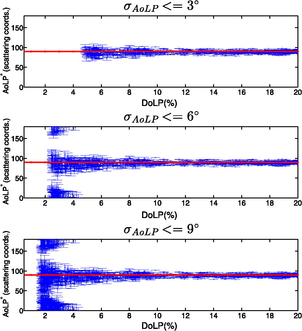$\pm 90 \deg$ .

To further investigate the presence of multiple scattering, Fig. 6(a) shows all AoLP measurements with a $\pm 2 σ_{AoLP}$ confidence interval that does not overlap the sky’s AoLP within a 12 deg boundary. This thresholding results in including 4% of the pixels and the location of these are displayed in Fig. 6(b). A higher density of intermediate AoLP values are seen as the DoLP decreases which would be expected for the AoLP of multiple scattering events.¹³ This analysis suggests the possibility that GroundMSPI is capable of detecting multiple scattering events and that a very low number of multiple scattering events is present in this scene but is not comprehensive enough to conclude that the intermediate population of AoLP values is caused by multiple scattering. Instead this analysis motivates further statistical AoLP studies on more polarimetric cloud images, as well as inspection of instrument calibration data to check whether the Gaussian noise assumption is valid. This cursory statistical analysis of MSPI cloud images is presented to motivate the usefulness of an analytic form for the AoLP variance when the linear Stokes parameters are uncorrelated and normally distributed with equal variance.

Fig. 6

(a) To distinguish multiple scattering, pixels with a $\pm 2 σ_{AoLP}$ confidence interval that do not coincide with the sky’s AoLP are displayed. The sky’s AoLP is defined as 90 deg or 180 deg within a 12 deg range. These intervals are denoted by the red horizontal lines. This thresholding results in including 4% of the pixels in the image. A higher density of intermediate AoLP values is measured as the DoLP decreases, which would be expected for the AoLP of multiple scattering events. AoLP measurements that are below the sky AoLP (plotted in blue) are more dense than above the sky AoLP (plotted in cyan). (b) The locations of intermediate AoLP values are displayed as an overlay of dots on the intensity image; blue or cyan denotes the measurements below or above the sky AoLP.

5. Conclusion

Here, we have provided an analytic form which relates the central moments of the AoLP to the Gaussian statistics of the linear Stokes vector. This expression yields a functional relationship between the measurement uncertainty in AoLP and the measurement uncertainty in DoLP. This is especially useful for high fidelity imaging polarimetry measurements of low DoLP scenes. In such an environment, simple Gaussian assumptions on the statistics of the AoLP are not valid because the high measurement precision of the AoLP statistics may contain useful information about the scene. Additionally, we have shown that a simple PE analysis underestimates the AoLP variance at extremely low DoLP values, but is accurate at DoLP values that are high relative to the Stokes measurement uncertainty. An example use of the analytic form on AoLP variance is presented for an example in imaging polarimetry.

Appendices

Appendix

Substituting Eq. (2) into Eq. (3) yields an expression for the AoLP central moments involving two integrals

Eq. (13)

〈 {(θ - \bar{ϕ})}^{α} 〉 = \frac{1}{π} e^{\frac{- {\tilde{\bar{d}}}^{2}}{2}} \int_{0}^{\infty} d \tilde{p} \tilde{p} e^{\frac{- {\tilde{p}}^{2}}{2}} \int_{\bar{ϕ} - π / 2}^{\bar{ϕ} + π / 2} d θ e^{\tilde{p} (\tilde{\bar{q}} \cos (2 θ) + \tilde{\bar{u}} \sin (2 θ))} {(θ - \bar{ϕ})}^{α} .

From Fig. 1, it can be seen that

\tilde{\bar{q}} = \tilde{\bar{d}} \cos (2 \bar{ϕ})

and

\tilde{\bar{u}} = \tilde{\bar{d}} \sin (2 \bar{ϕ})

. Using the equality

\cos (A) \cos (B) + \sin (A) \sin (B) = \cos (B - A)

and the change of variables

β = 2 θ - 2 \bar{ϕ}

allows the angular integral from Eq. (13) to be expressed as

Eq. (14)

\frac{1}{2^{α + 1}} \int_{- π}^{π} d β β^{α} e^{\tilde{p} \tilde{\bar{d}} \cos (β)} .

To represent

β^{α}

on the

[- π, π]

interval, the function can be expanded in a Fourier series

Eq. (15)

β^{α} = \sum_{- \infty}^{\infty} B_{n}^{α} e^{in β},

where the Fourier coefficients are defined by

Eq. (16)

B_{n}^{α} = \frac{1}{2 π} \int_{- π}^{π} d β β^{α} e^{- in β} .

This integral can be represented recursively for

n \neq 0

by integrating by parts

Eq. (17)

B_{n}^{α} = \frac{{(- 1)}^{n} π^{α - 1} i}{2 n} [1 - {(- 1)}^{α}] + \frac{α}{in} B_{n}^{α - 1}

and the integral can be solved for

n = 0

Eq. (18)

B_{0}^{α} = \frac{π^{α + 1}}{2 π (α + 1)} [1 - {(- 1)}^{α + 1}] .

When

α = 0

the integral in Eq. (16) simplifies to

Eq. (19)

B_{n}^{0} = \frac{1}{2 π} \int_{- π}^{π} d β e^{- in β} = δ_{n 0},

where

δ

is the Kronecker delta function. Since the Fourier coefficients have closed-form solutions, substituting Eq. (15) into Eq. (14) is helpful because it leads to an expression

Eq. (20)

\frac{1}{2^{α + 1}} \sum_{n = - \infty}^{\infty} B_{n}^{α} \int_{- π}^{π} d β e^{in β} e^{\tilde{p} \tilde{\bar{d}} \cos (β)}

that can be related to a modified Bessel function

Eq. (21)

I_{n} (x) = \frac{1}{2 π} \int_{- π}^{π} e^{x \cos (θ)} e^{in θ} d θ .

Now the integral expression over the angle is replaced by an infinite sum involving modified Bessel functions

Eq. (22)

\frac{2 π}{2^{α + 1}} \sum_{n = - \infty}^{\infty} B_{n}^{α} I_{n} (\tilde{p} \tilde{\bar{d}}) .

By substituting these results into Eq. (13), the AoLP central moments are

Eq. (23)

〈 {(θ - \bar{ϕ})}^{α} 〉 = \frac{1}{2^{α}} e^{\frac{- {\tilde{\bar{d}}}^{2}}{2}} \sum_{n = - \infty}^{\infty} B_{n}^{α} \int_{0}^{\infty} d \tilde{p} \tilde{p} e^{\frac{- {\tilde{p}}^{2}}{2}} I_{n} (\tilde{p} \tilde{\bar{d}}) .

Noting the recurrence relations for derivatives of modified Bessel functions

Eq. (24)

\frac{d}{d x} I_{n} (x) = \frac{1}{2} I_{n - 1} (x) + \frac{1}{2} I_{n + 1} (x)

and using integration by parts from page 259 of Ref. 15 leads to the equality

Eq. (25)

\int_{0}^{\infty} d \tilde{p} \tilde{p} e^{\frac{- {\tilde{p}}^{2}}{2}} I_{n} (\tilde{p} \tilde{\bar{d}}) = \frac{\tilde{\bar{d}}}{2} \sqrt{\frac{π}{2}} e^{\frac{{\tilde{\bar{d}}}^{2}}{4}} [I_{\frac{n - 1}{2}} (\frac{{\tilde{\bar{d}}}^{2}}{4}) + I_{\frac{n + 1}{2}} (\frac{{\tilde{\bar{d}}}^{2}}{4})] \forall n \neq 0 .

For $n = 0$ , relating the modified Bessel function to a Bessel function with a purely complex argument allows a solution using integration by parts

Eq. (26)

\int_{0}^{\infty} d \tilde{p} \tilde{p} e^{\frac{- {\tilde{p}}^{2}}{2}} I_{0} (\tilde{p} \tilde{\bar{d}}) = \int_{0}^{\infty} d \tilde{p} \tilde{p} e^{\frac{- {\tilde{p}}^{2}}{2}} J_{0} (i \tilde{p} \tilde{\bar{d}}) = e^{\frac{{\tilde{\bar{d}}}^{2}}{2}}

Substituting these integral solutions into Eq. (23) leads to Eq. (4) which is presented in the body of this paper. This analytic expression offers a solution for the central moments of the AoLP that involves an infinite series of modified Bessel functions to avoid evaluating the expected value over two integrals. This infinite series has been shown to be computationally useful because it converges relatively quickly as presented in Fig. 3(a).

Acknowledgments

This work is supported by NSF/CHE-1313892. Christine Bradley provided the GroundMSPI images and brought the application of AoLP analysis to distinguish single and multiple scattering to our attention. Discussions with Michael Garay, Anthony Davis, and David Diner of the Jet Propulsion Laboratory, California Institute of Technology improved the interpretation of GroundMSPI data.

References

1.

R. A. Chipman, OSA Handbook of Optics, 22.21 –22.35 McGraw-Hill, New York (1995). Google Scholar

2.

A. DasGupta, Asymptotic Theory of Statistics and Probability, Springer, New York (2008). Google Scholar

3.

D. ClarkB. G. Stewart, “Statistical methods of stellar polarimetry,” Vistas Astron., 29 (1), 27 –51 (1986). http://dx.doi.org/10.1016/0083-6656(86)90013-9 VASTA6 0083-6656 Google Scholar

4.

F. GoudailA. Bénière, “Estimation precision of the degree of linear polarization and of the angle of polarization in the presence of different sources of noise,” Appl. Opt., 49 (4), 683 –693 (2010). http://dx.doi.org/10.1364/AO.49.000683 APOPAI 0003-6935 Google Scholar

5.

J. Naghizadeh-KhoueiD. Clarke, “On the statistical behavior of the position angle of linear polarization,” Astron. Astrophys., 274 968 (1993). AAEJAF 0004-6361 Google Scholar

6.

K. L. Coulson, “Effects of reflection properties of natural surfaces in aerial reconnaissance,” Appl. Opt., 5 (6), 905 –917 (1966). http://dx.doi.org/10.1364/AO.5.000905 APOPAI 0003-6935 Google Scholar

7.

M. MishchenkoL. Travis, “Satellite retrieval of aerosol properties over the ocean using polarization as well as intensity of reflected sunlight,” J. Geophys. Res. Atmos., 102 (D14), 16989 –17013 (1997). http://dx.doi.org/10.1029/96JD02425 JGRDE3 0148-0227 Google Scholar

8.

S. O. Rice, “Mathematical analysis of random noise,” Bell Syst. Tech. J., 24 (1), 46 –156 (1945). http://dx.doi.org/10.1002/(ISSN)1538-7305c BSTJAN 0005-8580 Google Scholar

9.

J. L. Quinn, “Bayesian analysis of polarization measurements,” Astron. Astrophys., 538 A65 (2012). http://dx.doi.org/10.1051/0004-6361/201015785 AAEJAF 0004-6361 Google Scholar

10.

P. R. BevingtonD. K. Robinson, Data Reduction and Error Analysis for the Physical Sciences, McGraw-Hill, New York (1969). Google Scholar

11.

D. Dineret al., “Exploration of a polarized surface bidirectional reflectance model using the ground-based multiangle spectropolarimetric imager,” Atmosphere, 3 (4), 591 –619 (2012). http://dx.doi.org/10.3390/atmos3040591 2073-4433 Google Scholar

12.

N. PustJ. Shaw, “Digital all-sky polarization imaging of partly cloudy skies,” Appl. Opt., 47 (34), H190 –H198 (2008). http://dx.doi.org/10.1364/AO.47.00H190 APOPAI 0003-6935 Google Scholar

13.

A. Kokhanovsky, “Optical properties of terrestrial clouds,” Earth Sci. Rev., 64 (3), 189 –241 (2004). http://dx.doi.org/10.1016/S0012-8252(03)00042-4 ESREAV 0012-8252 Google Scholar

14.

A. MahlerD. DinerR. Chipman, “Analysis of static and time-varying polarization errors in the multiangle spectropolarimetric imager,” Appl. Opt., 50 (14), 2080 –2087 (2011). http://dx.doi.org/10.1364/AO.50.002080 APOPAI 0003-6935 Google Scholar

15.

F. Olveret al., NIST Handbook of Mathematical Functions, Cambridge University Press, Cambridge (2010). Google Scholar

Biography

Meredith Kupinski earned a BS degree in imaging technology from the Rochester Institute of Technology and both MS and PhD degrees in optical science from University of Arizona. She is an assistant research professor at the University of Arizona’s College of Optical Sciences working on statistical optics, imaging science, and probabilistic decision theory. She is the recipient of a Science, Engineering, and Education for Sustainability (SEES) fellowship from the National Science Foundation.

Russell Chipman received his BS degree from MIT and his MS/PhD degree in optical science from the University of Arizona. He is the co-PI of the Jet Propulsion Labs Multi-Spectral Polarimetric Imager, a candidate instrument for the global monitoring of aerosols from space to support measurements of the global energy balance for climate studies. He is a fellow of both OSA and SPIE and the 2007 recipient of SPIE’s Stokes award for polarimetry.

Eric Clarkson obtained a BA degree in mathematics, physics, and philosophy from Rice University, an MS degree in physics and a PhD degree in mathematics from Arizona State University, and an MS degree in optical sciences from the University of Arizona. He is a professor at the University of Arizona with joint appointments in the Department of Medical Imaging and the College of Optical Sciences. His research interests include statistical decision theory, statistical estimation, information theory, and image analysis.

CC BY: © The Authors. Published by SPIE under a Creative Commons Attribution 4.0 Unported License. Distribution or reproduction of this work in whole or in part requires full attribution of the original publication, including its DOI.

Citation Download Citation

Meredith Kupinski, Russell Chipman, and Eric Clarkson "Relating the statistics of the angle of linear polarization to measurement uncertainty of the Stokes vector," Optical Engineering 53(11), 113108 (12 November 2014). https://doi.org/10.1117/1.OE.53.11.113108

Published: 12 November 2014

Access the abstract

JOURNAL ARTICLE
7 PAGES

DOWNLOAD PAPER SAVE TO MY LIBRARY

GET CITATION

CITATIONS

Cited by 15 scholarly publications.

Explore citations on Lens.org

KEYWORDS

Polarization

Statistical analysis

Polarimetry

Clouds

Multiple scattering

Error analysis

Bessel functions

1.

Introduction

2.

Mathematical Results

Eq. (1)

Eq. (2)

Eq. (3)

Fig. 1

Eq. (4)

Eq. (5)

Eq. (6)

Eq. (7)

Eq. (8)

Eq. (9)

Fig. 2

3.

Computational Results

Eq. (10)

Eq. (11)

Eq. (12)

Fig. 3

4.

Example Application in Imaging Polarimetry

Fig. 4

Fig. 5

Fig. 6

5.

Conclusion

Appendices

Appendix

Eq. (13)

Eq. (14)

Eq. (15)

Eq. (16)

Eq. (17)

Eq. (18)

Eq. (19)

Eq. (20)

Eq. (21)

Eq. (22)

Eq. (23)

Eq. (24)

Eq. (25)

Eq. (26)

Acknowledgments

References

Biography

Show All Keywords

Keywords/Phrases

Search In:

Publication Years