|
|
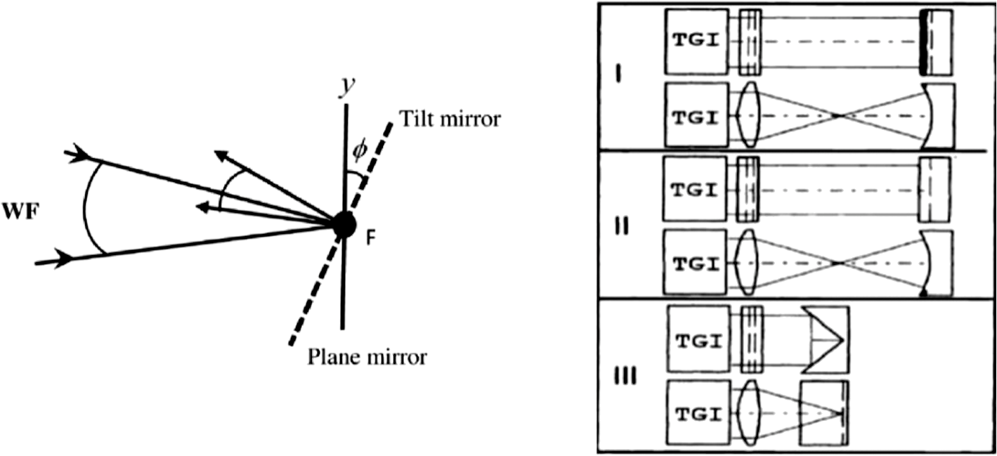
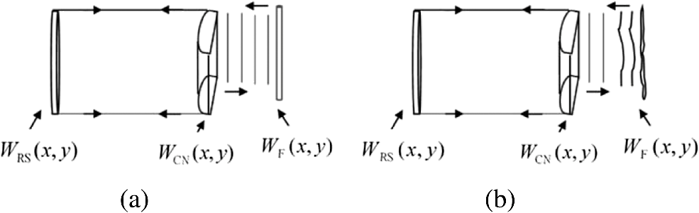
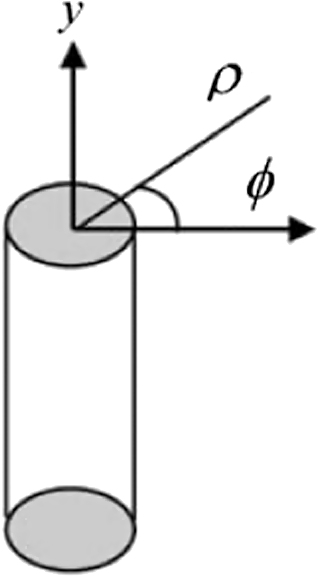
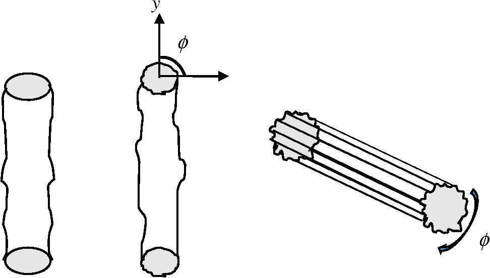
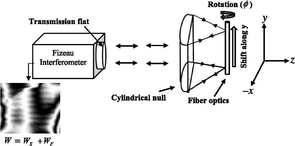
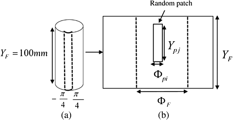
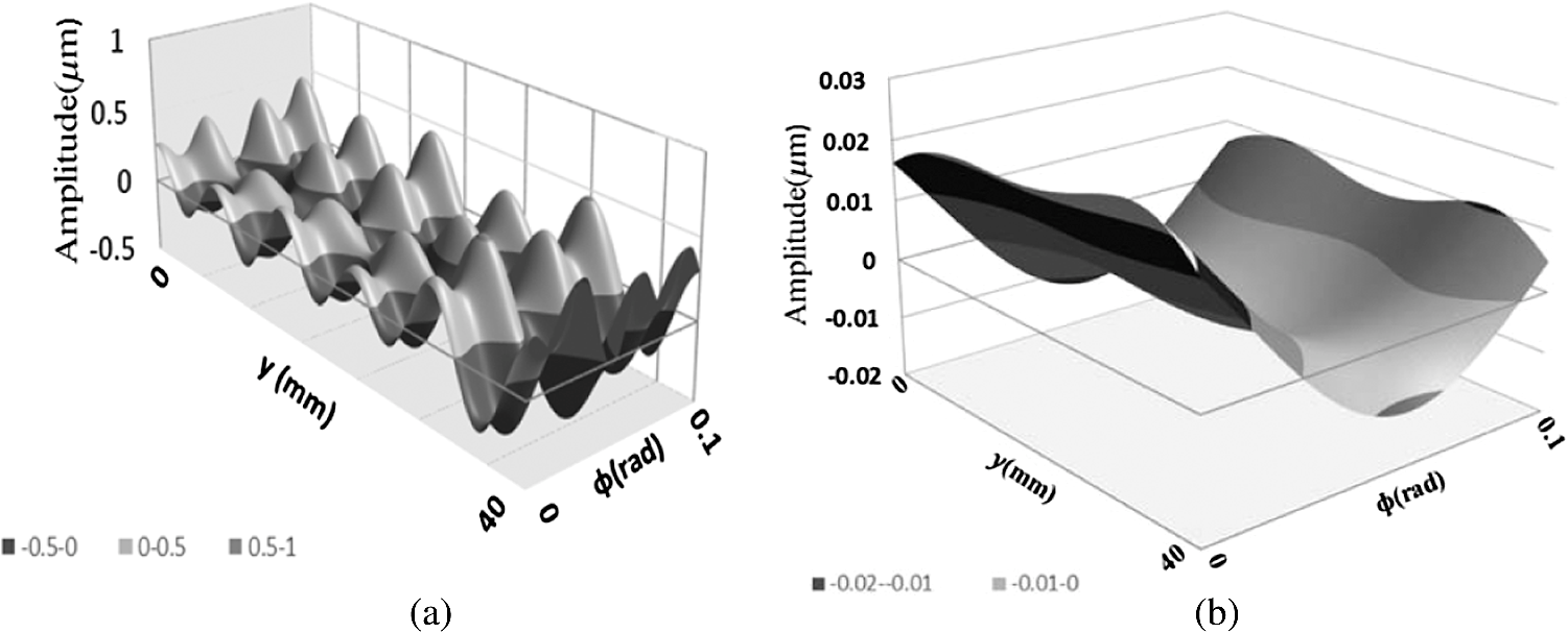
1.IntroductionIn interferometry, one endeavors to measure the deviation of the tested system as compared the ideal one. The real interferometric measurement includes the error of the tested surface plus any additional error caused by the interferometer system. In an interferometer measurement that has been set up well, the greatest remaining source of error is often the reference surface. This error can be the same magnitude or larger than the error of the optics to be tested, which reduces the measurement accuracy. To meet the demand for accurate interferometric test results, absolute measurement techniques have been used to separate the true surface deviation from the interferometric error. Absolute measurement of spherical surfaces has been well studied. These methods can be divided into two categories; calibrating the spherical reference surface and calibrating the tested part. Examples of the techniques to calibrate a spherical reference are the even/odd decomposition,1 symmetric/asymmetric decomposition,2 and the Cali ball averaging method.3–7 Techniques to calibrate the test part are rotationally and nonrotationally symmetric decomposition8 and also even/odd decomposition.9,10 From the review of the absolute testing method of spherical surfaces, it is apparent that these methods cannot be directly employed for absolute testing for cylindrical surfaces. Producing a high quality spherical surface reference is inherently easier than the producing similar cylindrical surfaces. Additionally, spheres are rotationally symmetric and have more degrees-of-freedom that do not change the reflected wavefront. The purpose of this paper is to present an absolute optical testing method that provides an efficient and accurate absolute measurement of cylindrical wavefronts. Section 2 briefly introduces the existing methods of cylindrical absolute testing. Section 3 describes the proposed method, Sec. 4 presents the simulation result and, finally, Sec. 5 describes preliminary experimental results. 2.Existing Absolute Testing Method of Cylindrical WavefrontCylindrical surfaces are a special case of a freeform surface; they are not rotationally symmetric. They have a powered axis as well as the plano axis or zero-power axis. The demand for such surfaces has increased in many applications such as laser scanning, laser diode collimation, as well as near-cylindrical surfaces such as grazing incidence x-ray optics and confocal domes. With the advances in fabrication processes for cylindrical surfaces, one of the looming challenges is to develop accurate surface measurement methods. Unfortunately, the desirable geometric shape is also the cause of testing difficulties. There are few techniques for the absolute testing of cylindrical surfaces. Two primary ones are described below. 2.1.Tilted MirrorThe principle of the first method is shown in Fig. 1(a).11,12 The cylindrical wavefront from the interferometer meets with a plane mirror. The plane mirror is placed at a cylindrical cat’s eye position, and is then tilted so the wavefront is reflected at different angles. By combining these wavefront-sheared measurements, the interferometer error contribution can be calculated. 2.2.Roof MirrorThis method is somewhat analogous to a method for absolute spherical surface testing.9 As illustrated in Fig. 1(b),12 three relative measurements are taken. By combining these three measurements, the interferometer error can be calculated. We note that for both of these methods, the reported measurement accuracy reached is . For the tilting mirror method, it is difficult to decouple tilt, focus, and lateral motion. Unless the mirror is rotated about the line focus, light will reflect off different areas of the mirror and each area will contribute a different error to each measurement. Another disadvantage of the tilting mirror method is that it reveals only the error as a function of , so only errors in the -direction are revealed. It is blind to any error correction in the direction. Hence, we propose a new technique for improving the accuracy of cylindrical optic testing based on the integration of two well-known techniques. 3.Proposed MethodThis approach is based on the merging of the random ball test method with the fiber optic reference test. The random ball test assumes a large number of interferograms of a good quality sphere with errors that are statistically distributed such that the average of the errors goes to zero.3–7 The fiber optic reference test utilizes a specially processed optical fiber to provide a high quality reference wave from an incident line focus from the cylindrical wave under test.13–16 By taking measurements at different rotations and translations of the fiber, an analogous procedure can be employed to determine the quality of the converging cylindrical wave with high accuracy—a “random fiber” test. 3.1.Analysis of Cylindrical Wavefront Error ContributionsThe proposed interferometer configuration and coordinate geometry for absolute testing of a cylindrical wavefront using fiber optics are shown in Fig. 2. Fig. 2Configuration for the absolute testing of cylindrical wavefront using fiber optics where the fiber is oriented along the -axis. 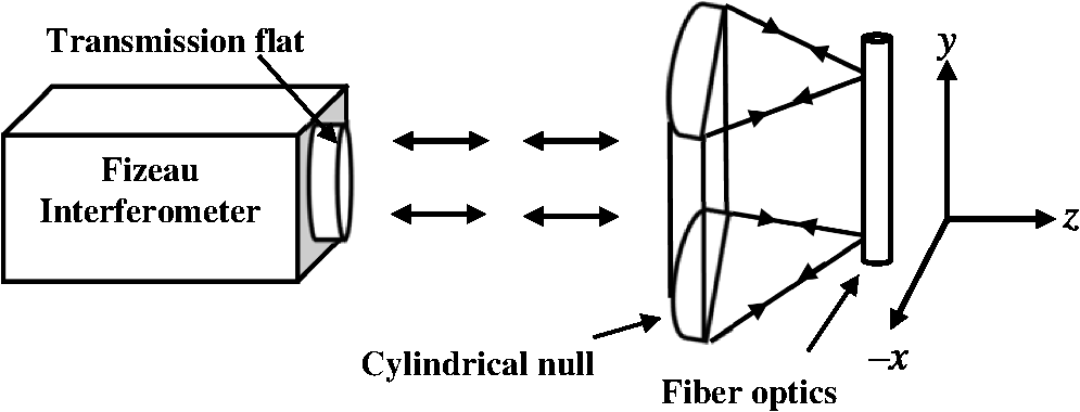 In the first pass, a collimated wavefront from the interferometer propagates to the cylindrical null optic. Then it passes through the null optic to be focused into a waist region extending along the surface of the fiber. When the fiber interacts with a collimated beam, only a small portion of the incident beam on the fiber will reflect back into the null13–16 due to the small radius of the reflective cylindrical fiber reference. The wavefront error sources of this experiment are described by considering two cases. 3.1.1.Case of ideal optical fiber referenceIn this case, the incident wavefront picks up the error of the flat reference, the cylindrical null, and then the fiber reference as shown in Fig. 3(a). Following Geary,13–16 the fiber filters the axis but passes the variation along the axis. Thus, the errors contribution of the wavefront reflected off the fiber can be written as where (the fiber wavefront error) is twice the fiber optic surface error. is the wavefront error of the transmission flat reference, and is the error of the cylindrical null. The wavefront returns through the null and picks up its error then interacts with the flat reference surface and picks up its error. Therefore, the measured wavefront can be written asEquation (2) reduces to where is the instrument error.For an ideal fiber optic reference surface, the fiber adds no wavefront error, thus Consequently, the total wavefront error sources in this case are 3.1.2.Case of nonideal optical fiber referenceWhen the fiber optic surface is not perfect, as shown in Fig. 3(b). The total wavefront error is described by Eq. (3). This imperfect wavefront reference adds unknown errors to the actual optical figure error measurement. For applications that require knowledge of the cylindrical wavefront to accuracies better than the fiber optic reference, it is critical to quantify and remove the fiber error contribution. In the following section, these errors of the fiber reference surface are decomposed in a way that enables the proposed approach to extract and remove these errors from the eventual measurement of the test part. 3.2.Decomposition of Possible Geometric Errors of the Fiber ReferenceCreating the fiber reference begins with the production of the optical fiber and ends with mounting it on its stage, and the surface irregularities are generated throughout the whole process. During the fiber drawing process there are several factors that cause variation in the fiber cladding diameter.17–20 To prepare the optical fiber as a reference, the plastic jacket is removed13 which may induce cracks, pulls, divets, or sharps microbends. The dejacketed fiber is then coated with reflective material, typically aluminum, but the coating uniformity is unknown. Finally, the fiber is gently stretched across a special mount, operating under tension to avoid sagging or bending.13 To discuss the form of potential geometric errors of the fiber reference, we first assume cylindrical coordinate symmetry about the fiber as illustrated in Fig. 4. Note that, to date, one publication has discussed the accuracy of using the fiber as a reference, stating only that the fiber is P–V or better.13 As cylindrical wavefront accuracy is typically quoted separately along the powered and the plano axes directions,21 there is a need for better data. We begin by defining four possible forms of geometric error on the fiber surface. The first three are fiber diameter variations , longitudinal error , and random bumps , Fig. 5. The tensioned fiber is effectively straight, so the fourth geometric error, bending, is assumed to be negligible and is ignored, though it could be accommodated with . 3.3.Measurement Algorithm DevelopmentThe proposed absolute interferometric testing is illustrated in Fig. 6. The fiber is precisely located at the cylindrical null focal line so the number of fringes is minimized in the test aperture. An interferogram is taken and the wavefront data stored. We start with the basic assumption that the measured wavefront is the sum of system error and fiber surface error According to Sec. 3.2, we can write as the sum of three wavefront error sources: Therefore, the measured wavefront in Eq. (5) can be written as Perfect cylindrical optics has three degrees-of-freedom that do not change the reflected wavefront. They are translation along the cylindrical axis, rotations about the -axis, and flipping the fiber . Based on this principle, we propose three steps to quantify and remove the fiber geometric error contribution from the actual measured wavefront. 3.3.1.Average of y-shifting tests of the fiberTo remove the fiber diameter variation, , one takes many measurements at different shifts. This is a one-dimensional (1-D) analogy to a Cali ball.3–7 The fiber optic is translated along its length various distances to get additional information about the fiber. The measured wavefront for each shift distance is where denotes one of many -shifts of the fiber. A series of these interferograms, averaged, yields where is the average of shifting measurements. and remain constant in all measurements, soThen the average of measurements reduces the wavefront errors in Eq. (9) to 3.3.2.Average of -rotation tests of the fiberTo remove the longitudinal error of the fiber, , we rotate the fiber about its center where the rotation is now a 1-D analog to the Cali ball test.3–7 In this step, the fiber is rotated around its axis , and each time it is rotated, an arbitrary new patch of the fiber surface is illuminated and produces a different wavefront measurement: where denotes one of many -rotations of the fiber. When a series of interferograms have been taken and averaged, following the same process as in the previous technique yields where is the average of -rotation measurements.3.3.3.Average of -rotation and y-shift tests of the fiberThis is the complete cylindrical analogue of the Cali ball test3–7 where the fiber is shifted and rotated randomly. The resulting wavefront measurement of each patch is An average over random rotations and shifts of the fiber is then described by The optical system error remains constant in all the measurements. Thus Subtracting Eq. (14) from Eqs. (10) and (12), we can get the fiber surface deformation error contribution to the actual wavefront measurement: And to get , we need only one measurement, so that at the position defined for measurement . Thus, we can now remove all errors introduced by the fiber reference and get absolute calibration of a cylindrical null or optic.4.SimulationA fiber reference test simulation of this calibration method, the complete cylindrical analogue of the Cali ball test,5 was performed to both validate the approach in reducing the effect of fiber reference errors, and to exercise the software algorithms needed for future experiments. 4.1.Fiber Error ModelingThe fiber cladding surface shape is unknown; no published papers discuss the diameter variation of the cladding, especially at the spatial periods over which we are interested. Additionally, the effect of de-jacketing and metalizing the optical fiber cladding is unknown. We, therefore, chose a simple model of fiber surface shape errors which matches the physically appropriate error decomposition described above. This allows us to both exercise and check our algorithms and conceptually prove the proposed method. The surface errors were described by the sum of sinusoidal errors in and each with random amplitudes and phase, and random Gaussian bumps or divits whose position, amplitude, and widths were also randomly generated: where , , and are the amplitudes and , represent the period and the phase shifting, respectively. The parameter and are the centers of the bump or divits and , is their width.We used parameters that match the pending experimental values. The total fiber length is and the range of rotation is . The long dimension of the cylindrical null in Fig. 6 is and it generates a cylindrical wavefront with . Thus, the size of each measurement patch on the fiber is and as shown in Fig. 7. 4.2.Result and DiscussionA series of 50 simulated fiber references surfaces, each with different spatial surface deformation, were randomly generated in order to evaluate the effect of applying this “random fiber” approach. Based on the only published data on the fiber reference quality and the fiber manufacturing tolerance of diameter, we have only accepted randomly generated surfaces which have no more than of error. Regardless of the magnitude of the error, what matters is the reduction resulting from the multiple measurements. From this simulation, we have found that this method reduces the contributed P-V and RMS error by a factor, on average, and , respectively. The best case yielded a reduction in the PV of and an RMS of , where the worst case yielded a reduction in PV of and an RMS of . One example of simulated fiber surface errors with a peak-to-valley distance and 0.18waves RMS along the entire fiber length is shown in Fig. 8. Simulation shows that the averaging of 231 patches leaves a residual fiber error of peak-to-valley, and an RMS error of . This is a reduction in P-V and a reduction in RMS compared to a single patch. Thus, this method appears feasible in eliminating the error contribution of the fiber reference to the measurement. 5.Preliminary Experimental ResultsA preliminary set of data was taken with a properly prepared fiber. This initial experiment only explores the average of the -shifting technique of the fiber due to limitations with the stages and some residual misalignment issues, as discussed in a recent article.22 A 40-mm cylindrical null23 was tested against a 100-mm-long fiber. The fiber was shifted vertically () in random steps of length to 30 different shift positions. The individual measurements, which all showed distinct differences indicative of fiber reference errors, were decomposed into Chebyshev polynomials in order to analyze the results.24 The 30 shifted measurements were averaged, and the individual measurements were then compared to the average. The PV and RMS error differences between the individual measured surfaces and the average were calculated. They ranged from a maximum of PV and RMS, to a minimum of PV and RMS. These are the errors, or uncertainties, in a calibration measurement based on only a single-fiber reference test. Additionally, as reported in Ref. 22, with this method, the uncertainties in a single-fiber reference test were expressed as Chebyshev polynomial terms, enabling detailed powered and plano axis descriptions of the errors. Finally, this preliminary -shifting experiment shows that the fiber reference errors can be significantly reduced. 6.ConclusionThe fiber optic reference combined with the principles of the random averaging method yield a technique for absolute interferometric testing of near cylindrical surfaces. We defined and decomposed the major potential error sources of the fiber reference surface that affect the measurement accuracy. With the new procedure and algorithm, the different error components of the fiber can be calculated and subtracted from the actual measurement of the cylindrical surface. Simulation and preliminary experimental results show that the proposed method should greatly improve high accuracy measurements of cylindrical surfaces. There are further experiments underway to quantify and eliminate the other fiber reference error components. Initial testing will first examine the misalignment errors resulting from the fiber reference itself. The authors are anticipating, and expect to soon publish, misalignment-induced aberration trends for a fiber reference. This will also speed fiber reference testing since misalignments will be numerically correctable. ReferencesR. Schreineret al.,
“Absolute testing of the reference surface of a Fizeau interferometer through even/odd decompositions,”
Appl. Opt., 47 6134
–6141
(2008). http://dx.doi.org/10.1364/AO.47.006134 APOPAI 0003-6935 Google Scholar
W. Songet al.,
“Absolute calibration of spherical reference surface for a Fizeau interferometer with the shift-rotation method of iterative algorithm,”
Opt. Eng., 52 033601
(2013). http://dx.doi.org/10.1117/1.OE.52.3.033601 OPEGAR 0091-3286 Google Scholar
U. Griesmannet al.,
“A simple ball averager for reference sphere calibrations,”
Proc. SPIE, 5869 58690S
(2005). http://dx.doi.org/10.1117/12.614992 PSISDG 0277-786X Google Scholar
R. E. Parks,
“A practical implementation of the random ball test,”
in Frontiers in Optics,
(2006). Google Scholar
P. ZhouJ. Burge,
“Limits for interferometer calibration using the random ball test,”
Proc. SPIE, 7426 74260U
(2009). http://dx.doi.org/10.1117/12.828503 PSISDG 0277-786X Google Scholar
Y. Zhouet al.,
“Application of the random ball test for calibrating slope-dependent errors in profilometry measurements,”
Appl. Opt., 52 5925
–5931
(2013). http://dx.doi.org/10.1364/AO.52.005925 APOPAI 0003-6935 Google Scholar
R. E. ParksC. J. EvansL. Shao,
“Calibration of interferometer transmission spheres,”
in Optical Fabrication and Testing Workshop OSA Technical Digest Series,
(1998). Google Scholar
W. SongF. WuX. Hou,
“Method to test rotationally asymmetric surface deviation with high accuracy,”
Appl. Opt., 51
(22), 5567
–5572
(2012). http://dx.doi.org/10.1364/AO.51.005567 APOPAI 0003-6935 Google Scholar
K. CreathJ. C. Waynt,
“Absolute measurement of spherical surfaces,”
Proc. SPIE, 1332 2
–7
(1990). http://dx.doi.org/10.1117/12.51045 PSISDG 0277-786X Google Scholar
K. CreathJ. C. Wyant,
“Testing spherical surfaces: a fast, quasi-absolute technique,”
Appl. Opt., 31 4350
–4354
(1992). http://dx.doi.org/10.1364/AO.31.004350 APOPAI 0003-6935 Google Scholar
G. Schulzet al.,
“Calibration of an interferometer for testing cylindrical surfaces,”
Opt. Commun., 117 512
–520
(1995). http://dx.doi.org/10.1016/0030-4018(95)00125-R OPCOB8 0030-4018 Google Scholar
K.-E. Elßneret al.,
“Absolute interferometric calibration of cylindrical surfaces: experiments,”
Proc. SPIE, 2536 75
–80
(1995). http://dx.doi.org/10.1117/12.218462 PSISDG 0277-786X Google Scholar
J. GearyL. Parker,
“A new test for cylindrical optics,”
Proc. SPIE, 661 359
–364
(1986). http://dx.doi.org/10.1117/12.938638 PSISDG 0277-786X Google Scholar
J. Geary,
“Data analysis in fiber optic testing of cylindrical optics,”
Opt. Eng., 28
(3), 283212
(1989). http://dx.doi.org/10.1117/12.7976936 OPEGAR 0091-3286 Google Scholar
J. Geary,
“Fiber/cylinder interferorneter test: focus and offaxis response,”
Opt. Eng., 30
(12), 1902
–1909
(1991). http://dx.doi.org/10.1117/12.56022 OPEGAR 0091-3286 Google Scholar
J. Geary,
“An overview of cylindrical optics testing using a fiber optic reference,”
Proc. SPIE, 2536 68
–74
(1995). http://dx.doi.org/10.1117/12.218461 PSISDG 0277-786X Google Scholar
S. E. MillerI. P. Kaminow, Optical Fiber Telecommunications, Academic Press, Boston
(1998). Google Scholar
J. F. Owenet al.,
“Determination of optical-fiber diameter from resonances in the elastic scattering spectrum,”
Opt. Lett., 6 272
–274
(1981). http://dx.doi.org/10.1364/OL.6.000272 OPLEDP 0146-9592 Google Scholar
M. H. Weik, Fiber Optic Standard Dictionary, Van Nostrand Reinhold, New York
(1997). Google Scholar
P. ReardonA. Alatawi,
“Experimental results for absolute cylindrical wavefront testing,”
Proc. SPIE, 9206 92060E
(2014). http://dx.doi.org/10.1117/12.2062320 PSISDG 0277-786X Google Scholar
P. ReardonF. LiuJ. Geary,
“Schmidt-like corrector plate for cylindrical optics,”
Opt. Eng., 49
(5), 053002
(2010). http://dx.doi.org/10.1117/1.3421652 OPEGAR 0091-3286 Google Scholar
F. Liuet al.,
“Analyzing optics test data on rectangular apertures using 2-D Chebyshev polynomials,”
Opt. Eng., 50
(4), 043609
(2011). http://dx.doi.org/10.1117/1.3569692 OPEGAR 0091-3286 Google Scholar
BiographyAyshah Alatawi is currently pursuing her PhD degree in electrical engineering at the University of Alabama in Huntsville. In 2010, she received her MS degree in physics from the University of Alabama in Huntsville. Her current research interest is optical metrology of freeform optics. She is a member of SPIE. Patrick J. Reardon is the associate director of the Center for Applied Optics and an assistant professor in the Electrical Engineering Department at the University of Alabama in Huntsville. His research has covered the fields of optical design, fabrication and testing for DoD, aerospace, ophthalmic, and commercial applications. |