|
|
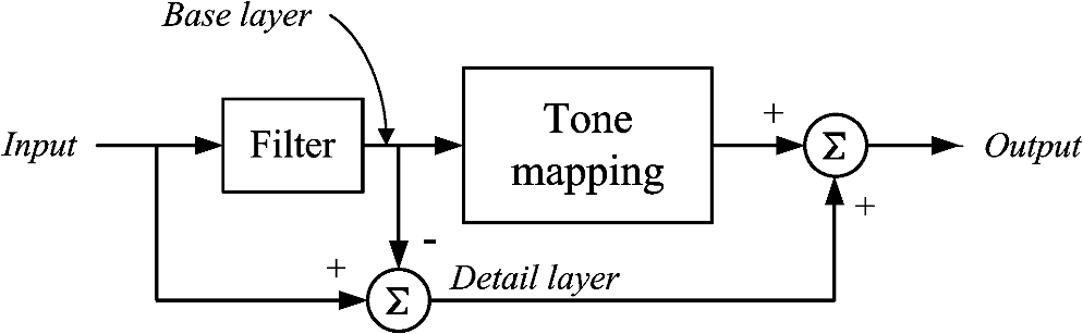
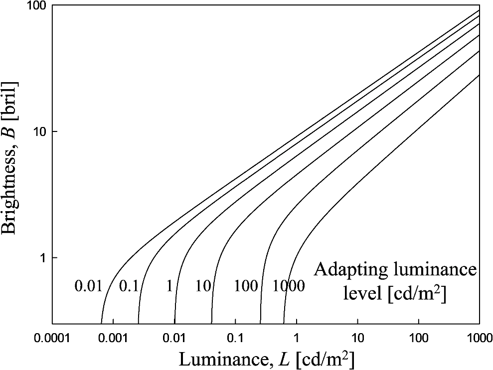
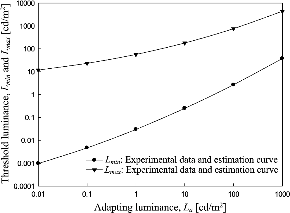
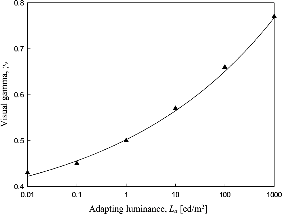
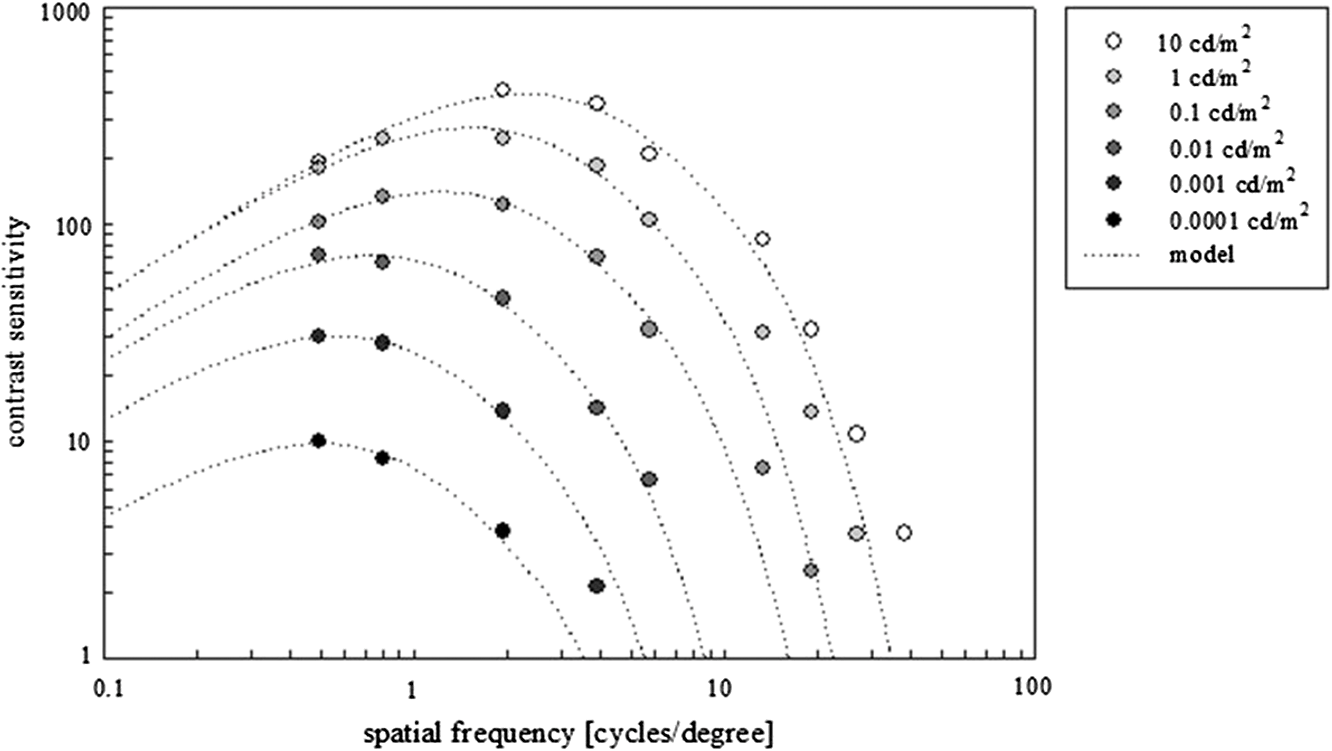
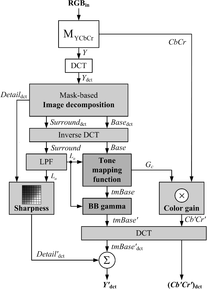
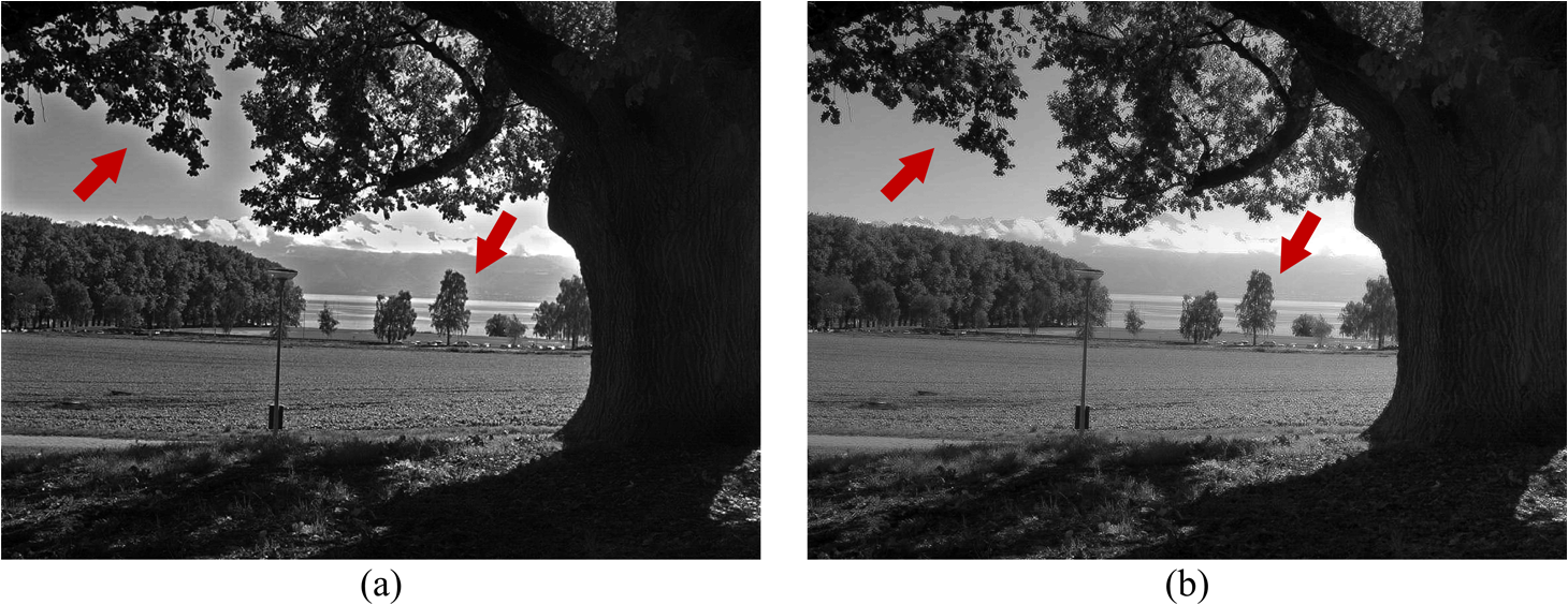
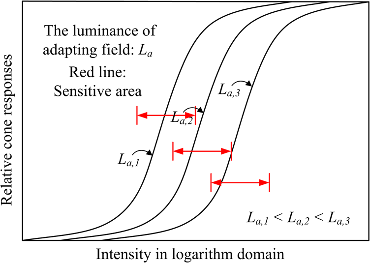
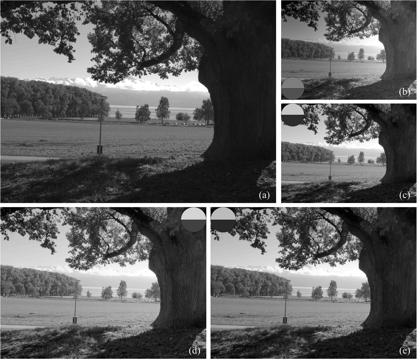
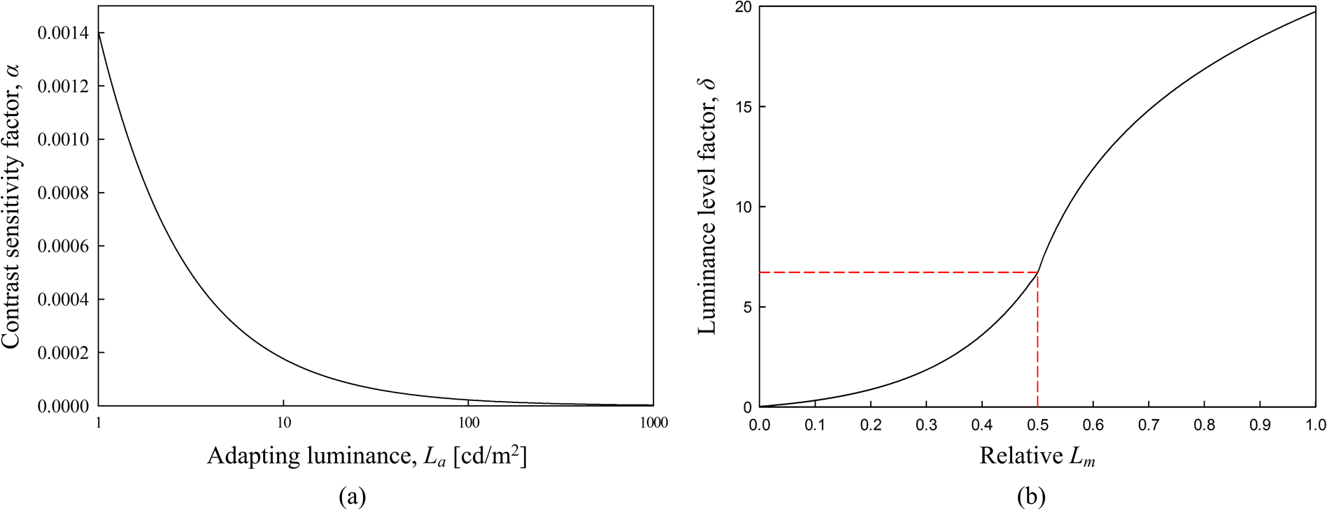
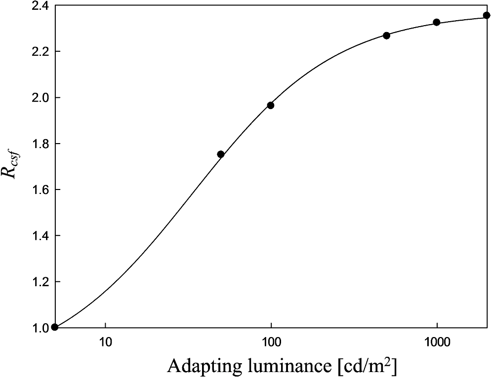
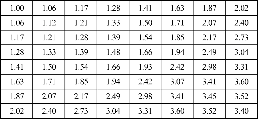
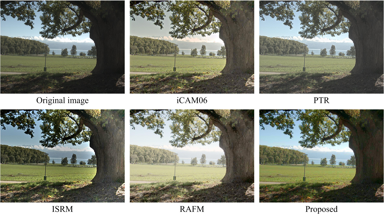
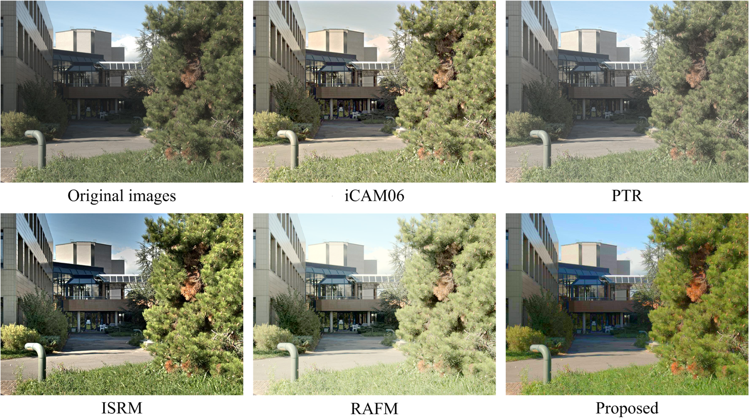
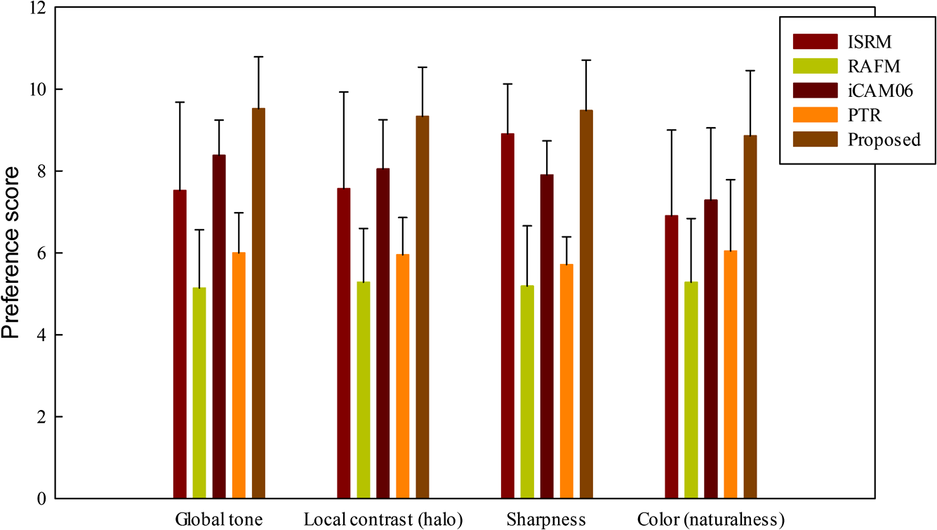
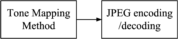
1.IntroductionThe luminance dynamic range in the real world is significantly large and the dynamic range of the eyes can shift in response to the change or intensity of scenes.1 In contrast, image sensors that capture the luminance dynamic range are limited to a certain intensity range, which is relatively very low. Thus, there is a substantial difference between an image captured by a sensor and the perceived scene.2 To reduce this discrepancy, researchers have proposed a number of global and local tone mapping methods. The global tone mapping method using only one mapping function has a relatively simple computation, though it is insufficient to address wide dynamic range, whereas the local tone mapping method has an adaptive function that may vary depending on spatially adjacent pixels. Furthermore, certain local methods adopt human visual properties for local contrast enhancement, such as image color appearance model (iCAM)-based methods,3,4 logarithmic mapping,5 local eye adaptation,6 and histogram adjustment.7 These make images similar to real scenes that an observer would perceive. It is widely known that human vision responds to luminance in such a manner that individual visual cells adjust each gain according to locally adapted luminance. Moreover, various experiments that help us understand the instinctive nature of human vision have been conducted by psychophysicists. The results of the experiments are usually statistical data and need to be created as the functions so that they are easy to use. Recently, tone mapping operators are extended into video streams.8,9 These methods use temporally close frames to smooth out abrupt changes of luminance.10 In addition, for surveillance system, content-based tone mapping has been proposed.11 It presents inter and interframe object based tone mapping for the enhancement of regions of interest (ROIs) in video streams. Essentially, this content-based method has piecewise global tone mapping based on features from detected ROIs. Generally, local tone mapping methods have better performance because the human visual system is a spatial correlation system sensitive to regional relative brightness, rather than a system described globally single tone curve.4 Local tone mapping methods usually use image decomposition for edge preservation. Textures and detail information can be removed when a dynamic range is largely compressed.3,12,13 The procedure for local tone mapping using image decomposition is shown in Fig. 1. The detail layer is preserved, whereas the base layer is compressed by tone mapping. The base layer has large features and is extracted by filtering the input image. The detail layer is a subtraction of the base layer from the input. After compressing the base layer, it is recomposed with the detail layer. The details are not suppressed through tone mapping. Therefore, image decomposition is a necessary procedure for local tone mapping methods. This paper proposes a luminance-adaptive local tone mapping method in the compression field for the contrast enhancement of low dynamic range images. Tone mapping is composed of simple local functions related to human vision properties that respond to luminance change. In order to achieve this, we investigate human visual sensitivity properties using two luminance adaptation functions for simple or complex stimuli and contrast sensitivity functions (CSFs). Our image enhancement is based on these luminance-adaptive human factors. In addition, we propose a novel image decomposition method in the compression domain using discrete cosine transform (DCT) band splitting. The image decomposition is not only a necessary step for local tone mapping, but also an initial step required for merging the proposed tone mapping with JPEG baseline. The previous spatial domain based methods require several Gaussian kernels for multiscale tone mapping and detail-base separation. Moreover, edge stopped blurring techniques to prevent halo artifact are computationally intensive.13 The proposed method does not use any Gaussian kernel for edge preserving and reduces the complexity of the process for adjusting sharpness and colors by cooperating with DCT coefficients. Consequently, it performs well in terms of simplicity of the process, detail preserving, tonal rendition, and halo artifact elimination. Further, for postcomplementary processing, mask-based sharpness enhancement, visual gamma correction, and color compensation are accomplished. The remainder of this paper is organized as follows. In Sec. 2, we discuss the luminance-adaptive human factors relevant to our research. In Sec. 3, we present the proposed algorithm for image contrast enhancement using mask-based image decomposition and luminance-adaptive local tone mapping. In Sec. 4, we describe complementary processes adopted for further image enhancement. In Sec. 5, we present simulations and comparative results. Finally, in Sec. 6, we provide concluding remarks. 2.Luminance-Adaptive Human Vision FactorsHuman vision accommodates variations in luminance through a process called light adaptation. In this section, we focus on three human factors in light adaptation: two types of brightness functions, proposed by Stevens and Stevens14 and Bartleson and Breneman,15 and contrast sensitivity functions.16 The brightness function represents the nonlinearity between perceived brightness and measured luminance of the same patch under various intensities of adapting luminance. According to the brightness function proposed by Stevens, brightness is increased sharply when human vision perceives the luminance of a patch to be increasing from darkness. It changes linearly over the threshold as shown in Fig. 2 on a logarithmic scale. Moreover, the slope and threshold of a linear area increase with adapting luminance. In other words, in order for the perceived contrast ratio with brightness to be preserved, the physical contrast ratio with luminance is decreased with an increase of adapting luminance. In contrast to the simple patch experiments conducted by Stevens, Bartleson and Breneman conducted experiments to predict the brightness for a complex stimulus. According to the results by Bartleson and Breneman, brightness perceptions of complex scenes, such as images, can be described by both a power term and an exponential decay term. Human vision is more sensitive to change or difference than the absolute value of luminance. Generally, image having a high contrast ratio is more distinct at lower levels of adaptation.17,18 However, because of nonlinearity between perceived brightness and measured intensity under different adaptations, it is impossible to fix the physical contrast ratio that is suitable for an image with various intensity ranges. To address this problem, Lee et al. obtained a curve representing the relation between threshold luminance and adapting luminance for constant brightness perception using the Stevens’ results and Bartlenson–Breneman’s functions.19 As shown in Fig. 3, the curve represents the highest and lowest luminance perceived by human vision at each adapting luminance. Based on these extreme luminance values, the necessary contrast ratio at each adapting luminance is shown in Fig. 4. For an identical perception of a certain contrast ratio, human vision requires a high luminance ratio at a low adapting luminance, and vice versa; it requires a relatively low luminance ratio at a high adapting luminance. In addition, to apply this nonlinearity to Bartleson–Breneman’s functions, Lee et al. proposed visual gamma estimation for varying adaptation shown in Fig. 5. This shows that the exponent of the intensity function increases with increasing adapting luminance. Photographic images require gamma correction based on the estimated visual gamma. Additionally, we examine the properties of the CSF of human vision. The CSF specifically refers to the relation between contrast sensitivity and spatial frequency. In general, the CSF is measured by grating patterns that have changeable contrast and spatial frequencies. Contrast sensitivity is an inverse of the detection threshold where the contrast of a grating pattern cannot be perceived.20 As a related study, there is the experiment of van Meeteren and Vos.16 According to their experiment, human vision is more sensitive to the contrast of grating patterns in high adapting luminance. Furthermore, for higher adapting luminance, contrast sensitivity is saturated. Figure 6 shows the results of van Meeteren and Vos. The CSF has band-pass shape and the maximum value of the CSFs increases for higher adapting luminance. 3.Proposed AlgorithmThe proposed tone mapping method is integrated with the procedure for baseline encoding in JPEG to ensure that the input for tone mapping is not degraded. The method is located between DCT and quantization in JPEG encoding. The overview of the proposed method is shown in Fig. 7. An input image has RGB color channels and color conversion from RGB to YCbCr.21 In the compression field, the component is decomposed into , , and . is necessary to calculate the local adapting luminance . and represent the base layer and detail layer, respectively. After mask-based image decomposition, Base is developed into by applying luminance-adaptive tone mapping functions according to the Surround value; then, and are enhanced with respect to sharpness, gamma, and color. The enhanced and are combined into , which can continue with the JPEG baseline. The chrominance components CbCr are simply compensated by color gain . 3.1.Mask-Based Image DecompositionAdaptive spatial filtering, such as the bilateral filter and sub-band coding by Laplacian pyramid, have been introduced for image decomposition.13,22–24 These methods usually have computational complexity and calculation burdens.4 In JPEG baseline, DCT coefficients include information for extracting sub-band images, which represent detail, base, and surround.25 In this study, a simple method of implementation for image decomposition in the compressed field is proposed. For detail preservation, an image is separated into two layers: detail layer and base layer, which represent the local texture and large features, respectively. The detail layer represents local high-frequency components and the base layer represents low-frequency components locally. This is shown in Fig. 8. The input image is decomposed using the bilateral filter. It shows the characteristics of the base layer and detail layer, which represent locally blurred images and local textures, respectively. Fig. 8Images decomposed using the bilateral filter: (a) input image, (b) base layer, and (c) detail layer.  In JPEG baseline, DCT coefficients are computed within an block. An image is converted from the spatial domain to the frequency domain with an block size. Thus, it is possible to separate frequency components locally by splitting DCT coefficients in the block. Figure 9(a) shows the DCT block and location of coefficients for band splitting. The top-left coefficient is a direct current (DC) component of the block image. We assign a DC component to the surround layer, set DC and the low-frequency components into the base layer and high-frequency components into the detail layer. This image decomposition is implemented with a masking method. Figures 9(b) and 9(c) are macro masks for extracting the base layer and detail layer. The use of DCT allows the integration of local tone mapping in JPEG baseline. Fig. 9Mask-based image decomposition in discrete cosine transform (DCT) block: (a) DCT block, (b) mask for base layer, and (c) mask for detail layer. 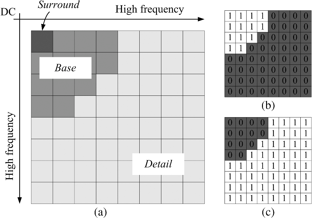 For analysis of the proposed DCT mask, we compare a DCT mask and bilateral filtering to separate base and detail layers. Detail layer images through bilateral filtering and DCT mask splitting are shown in Fig. 10. Blurring is distributed throughout strong edges across foreground regions (trees) and background regions (sky and grass). As a result, a halo artifact occurs around strong edges. Blurred white outlines near edges in the detail layer from bilateral filtering causes the halo artifact. In contrast, because a proposed detail separation is conducted in an DCT block, the region where halo artifacts appear could not be larger than an block. For pair comparison, tone mapped images are produced by the same tone mapping operator (TMO) for each separated base layer. As shown in Fig. 11, the halo artifacts differentially appear in result images. A DCT masking method, consequently, leads to diminished halo effects. 3.2.Luminance-Adaptive Tone Mapping for the Base LayerSome tone mapping functions are based on an electrophysiological model that predicts the response of photoreceptors (rods and cones) at any adaptation level.6 This has usually been adopted by other authors to model perceived brightness; also, our tone mapping function is based on this model. The shapes of functions are similar to an S-shaped curve in the logarithm domain.26,27 The basis function is given by where and are the intensities of input and output images, respectively, and and are the parameters for the S-shaped formulation.This basis function has been inspired by a power-function response in CIECAM02 (Ref. 28), which presents the postadaptation nonlinearities of cone responses. Figure 12 shows a relation between luminance intensity and cone responses for different adapting luminances. If the adapting luminance is high, cone responses are right-shifted. Cones change their sensitive area to a higher-intensity region for a higher adapting luminance. This processing, called as luminance adaptation, is enacted in local cones on the retina. This is the reason that cone responses are applicable in local tone mapping. A proposed tone mapping function follows the basis function, Eq. (1), with luminance adaptation processing. From Eqs. (2) to (6), analyzed brightness sensitivity properties are applied to local tone mapping. The proposed parameters are based on Stevens’ brightness functions and the analysis conducted by Lee et al. Tone mapping functions are given by where is a compression level factor, is a luminance level factor, is a contrast sensitivity factor, is a weighting factor, and is a mid-point value of . is a local white luminance map, is a local adapting luminance map, and is relative global luminance, which is an average value of normalized . accounts for the slope of the function, which is user-controllable and experimentally defined as 0.6 here. It is similar to that of CIECAM02 but modified for higher overall contrast.In Eq. (3), the compression level factor, , is defined as the degree of local compression. It has been formulated only for controlling the compression level without overall tone changing. In the threshold luminance analysis shown in Fig. 3, for identical contrast ratio perception under separate adapting luminance, the physical contrast ratio must increase for a lower adapting luminance. This is because the human visual system is more sensitive to luminance change when the adapting luminance is lower, so a higher physical contrast ratio is needed to keep local detail consistent in a dim surround viewing. In other words, to perceive a consistent brightness contrast regardless of variations in the adapting luminance, the image contrast should change in an exponential decay toward the higher adapting luminance. First, a contrast sensitivity factor, , which is a basic factor of , determines the contrast range of the image. It is derived from the physical contrast ratio according to the relative adaptation luminance at each white luminance in Fig. 4. It depends on the property that a high contrast ratio is required at a low adapting luminance, whereas at a high adapting luminance, a relatively low contrast ratio is sufficient. is set to 0.2 . is obtained from a Gaussian-blurred intensity image in which the max luminance is set to for outdoor scenes. In order to calculate , DC coefficients in DCT blocks are used, which are represented as in Fig. 6. Then, is weighted by factor of Eq. (5). A weighting factor, , is designed to meet the compression balance and prevent intensity saturation at higher or gray out at lower . restricts a compression range at higher and lower adapting luminances. Here, to reduce the effect on the average luminance of an image by , a mid-point value of the overall is fixed. In Eq. (6), the luminance level factor, , is designed to properly adjust an average luminance level of a resulting image, based on the analysis of average luminance for consistent brightness perception in Fig. 13. In viewing scenes with uniform luminance distribution from dark to bright, the average luminance values will have a linear relationship with the adapting luminance, which is defined as of the white luminance value of each scene. However, the human visual system has a nonlinearity property to perceive average luminance for adapting luminance. Figure 13 shows the difference between the physical average luminance and the perceived average luminance. A bold line represents median luminance values from visual threshold luminance values of Fig. 3 and a dashed line shows the physical average luminance for a uniform luminance distribution. From the analysis, although adapting luminance linearly changes, the perceived average luminance is not proportional to the changing ratio of the adapting luminance. This means that as the adapting luminance is lowered, human visions need a relatively higher average luminance than physical luminance to preserve average brightness; on the other hand, a relatively lower average luminance is needed for higher adapting luminance. The larger generates a lower average luminance level in the output image. On the contrary, if an image is exposed for a short period, the small makes the output image brighter. The parameter, , is derived based on the ratios between the values of bold and dashed lines for various adapting luminances; then it is adjusted using images with broad adapting luminance ranges. Figure 14 provides the resulting images with different values of and . First, the compression level factor controls the overall dynamic range of the image. For a higher (weighting factor : 2.5), the dynamic range of a represented image is more compressed (the bright portions are dimmed and the dark portions are lightened), whereas for lower values of (weighting factor : 0.5), the compression is lower. Figure 14(c) has a smaller value than Fig. 14(b), and the dynamic range of Fig. 14(c) is larger than Fig. 14(b). is formulated for applying the visual contrast characteristic to a tone mapping function according to Lee’s analysis for Stevens’ brightness function, which is shown in Fig. 4. Human vision requires a higher contrast ratio at a relatively lower adapting luminance,. Second, a luminance level factor effectively corrects an underexposed or overexposed image. The represented image is toned down for a high mean value of the input image based on the experimental results of Fig. 3. As shown in Figs. 14(d) and 14(e), the change of affects the average luminance of the output image. Based on this analysis, the factor is formulated for cooperating subjective experiments. These two fitted functions in Eqs. (5) and (6) are shown in Fig. 15. 4.Additional Processing for Image Enhancement: Gamma, Sharpness, and Color4.1.Visual Gamma CorrectionOverall tone reproduction through TMOs changes brightness contrast in images and the perceived lightness (or relative brightness) also changes as a function of different surround luminance.1,19 In the experimental results of Bartleson and Breneman for complex stimuli, the exponent of the lightness function increases with increasing adapting luminance, so photographic images require gamma correction based on the estimated visual gamma. Photographic images typically viewed in dim surroundings are reproduced using a power function with a lower exponent value. Based on this, Lee et al. proposed the visual gamma given by The visual gamma as a function of the adapting luminance means that gamma correction should be conducted adaptively with local luminance as for human vision. Therefore, we adopt the visual gamma as postprocessing after the proposed tone mapping. The output of tone mapping, , is gamma corrected according to the following equation: 4.2.Sharpness EnhancementIn order to compensate sharpness loss by the procedure for JPEG baseline, we apply CSF-based sharpening gain, , to an existing mask-based unsharpening method. CSF refers to the reciprocal of the minimum contrast ratio that human vision can perceive at each spatial frequency. In JPEG baseline, the sharpness enhancement is applied adaptively by luminance adapting the CSF properties based on the mask-based sharpness filter. We consider the contrast sensitivity of human vision for which a high contrast sensitivity means that objects are clearly visible. In order to design , we compute the relative contrast sensitivity as a function of adapting luminance using certain maximum values at each adapting luminance: 5, 50, 100, 500, 1000, and . The maximum contrast sensitivity at is set as a reference point. Figure 16 shows the ratio of maximum values to the reference at each adapting luminance. The proposed gain, , is fitted with a rational function using these points, which is given by The basis of the sharpness mask, , is shown in Fig. 17.29 The final sharpness enhancement using the CSF properties is given as follows: where is a detail layer that is decomposed using a mask-based image decomposition.4.3.Color CompensationGenerally, during the tone mapping with a simplified s-curve, the ratio of RGB signals changes and color saturation would be reduced.30 Although local tone mapping is applied to only the luminance channel, dynamic range compression generally results in an alteration of the ratio of chromatic channels and a reduction of color saturation. To correct this chronic defect of tone mapping, we adopt a simple method for color compensation which restores a ratio of color to luminance before tone mapping.30 This method is given by where the color gain is designed to preserve the ratio and a user-controlled factor , which prevents oversaturation, is experimentally determined as 0.45. In our experiment, the user-controlled factor of 0.45 is set for minimizing modified CIEDE2000 between reference images and proposed images. Modified CIEDE2000 considers only the hue and chroma differences between these images.315.Simulations and Results5.1.Objective and Subjective AssessmentTo conduct quantitative comparisons of the proposed method with existing tone mapping methods, several image assessment tools were employed, including the universal image quality index32 (UIQI), the no-reference perceptual quality assessment33 (NRPQA), the colorfulness metric ratio34,35 (CMR), and structural fidelity of tone mapped images36 (S). According to the mathematical definition of UIQI, the closer the UIQI value is to one, the better is the image quality. Unlike UIQI, NRPQA does not need a reference image, as it is aimed specifically at no-reference quality assessment of JPEG compressed images considering blurring and blocking as the most significant artifacts. As such, it is suitable for DCT-based image evaluation. A higher NRPQA value indicates a better image quality. CMR indicates the extent of color in the resulting image relative to the reference image. indicates local structural fidelity measure based on structural similarity (SSIM),37 which contains three comparison components: luminance, contrast, and structure. Compared with SSIM, the luminance comparison component is missing in since TMOs locally change original intensity. Using all four of these numerical assessments, we compared the proposed method with previous approaches, such as iCAM06,3 a photographic tone reproduction based on dodging and burning with a zone system33 (PTR), integrated surround retinex model38 (ISRM), and retinex-based adaptive filter method39 (RAFM). Resulting images for these methods are shown in Figs. 18Fig. 19Fig. 20–21. Evaluation results for the full set of images are shown in Fig. 22. Note that according to UIQI results, the proposed method trails PTR by a slight margin, but it is competitive with other methods. NRPQA, which is a perceptual assessment for JPEG compressed images, presents a more objective evaluation than UIQI. Note that the proposed method has the best NRPQA scores among all methods tested. The best score is assigned to the most robust method about blurring and blocking artifacts. According to CMR scores, the proposed method shows comparatively good performance and no halo artifacts, as is apparent in images processed using ISRM. Finally, from S scores, it is confirmed that the proposed method has structural fidelity equal to or higher than those of the other methods. Fig. 22Evaluation results using three metrics: universal image quality index, no-reference perceptual quality assessment, colorfulness metric ratio, and structural fidelity of tone mapped images. 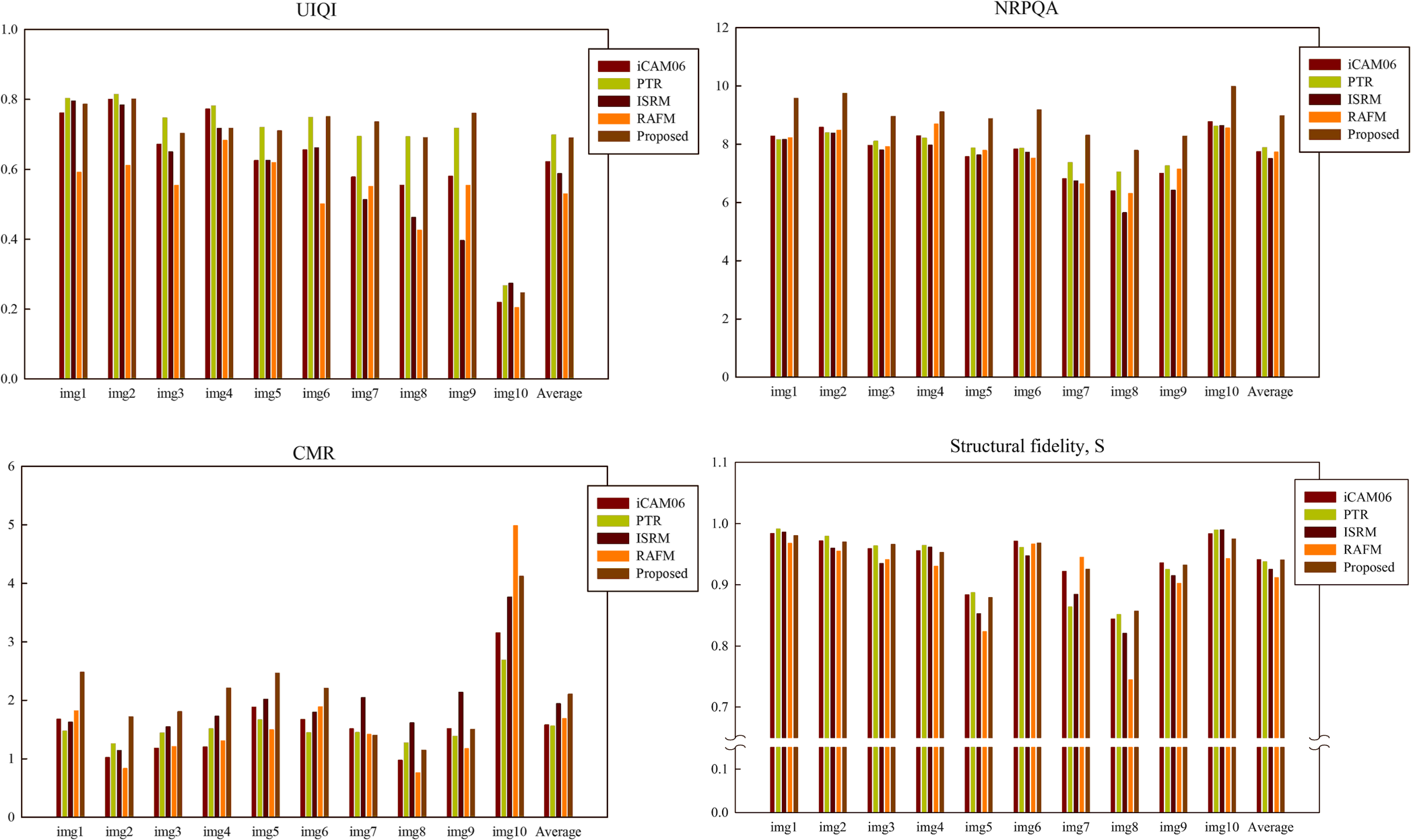 In addition to objective evaluation, we conducted the psychophysical experiment based on score rating. An original image is first presented; then reconstructed images by each method on a gray background are simultaneously shown on a display device: LG 47LM6700. Participants in the experiment are instructed to rate a score with 0-to-10 range for each attribute: global tone, local contrast (halo), sharpness, and color (naturalness). In the experiment, the total number of collected scores is . The average scores and standard deviations are presented as color bars and error bars in Fig. 23, respectively. The result shows that the proposed method is highly rated on the psychophysical experiment. Our overall assessment, based on qualitative comparison of the entire set of test images, confirms that the proposed tone mapping method produces colorful, high-contrast images with strongly enhanced details. In addition, according to subjective comparison, the proposed method has good preference scores for four-view, such as global tone, local contrast, sharpness, and color. All resulting images by the proposed method and the original images are shown in Fig. 24. 5.2.Computation TimeWe compute the computation time of the methods with the test setup as shown in Fig. 25. Considering the novelty of the proposed method that is inserted in JPEG baseline, JPEG encoding and decoding are conducted after tone mapping for the previous methods. For different resolutions (, , ), computation times in MATLAB® are listed in Table 1 (CPU: Intel i7-2600K 3.40 GHz, RAM: 4 GB). In Table 1, the computation time of our method is faster than those of iCAM06 and RAFM, but similar to those of PTR and ISRM. Compared with iCAM06 and RAFM adopting time-consuming tasks for edge preserving and anti-halo, such as the bilateral filter and anisotropic Gaussian functions, our method improves the edge resolution and halo artifact while saving a lot of computation time. Table 1Computation time of methods in MATLAB® (in seconds).
6.ConclusionsA novel approach to enhance images using tone mapping in the compression domain was presented. In order to combine tone mapping with JPEG baseline, we decomposed an image using mask-based DCT band splitting and suggested the luminance-adaptive tone mapping function, which was based on the brightness and contrast adaptation of human vision. For image application, we adopted the Stevens’ and Bartleson and Breneman’s experimental results and correlated analysis in order to mimic human vision properties. In addition, the procedure involved sharpness enhancement based on contrast sensitivity functions and color compensation. For the evaluation results, the performance of the proposed method was compared with previous approaches through several image assessment methods. It was discovered that the proposed method outperformed previous approaches in most cases. For optimal tone rendering, we are certain that the proposed method can be useful in physical still cameras in order to compress the dynamic range in JPEG baseline. AcknowledgmentsThis research was supported by Basic Science Research Program through the National Research Foundation of Korea (NRF) funded by the Ministry of Education (2012-R1A1A2008362). ReferencesM. D. Fairchild, Color Appearance Models, 2nd ed.John Wiley & Sons, Ltd., Chichester, United Kingdom
(2005). Google Scholar
E. Reinhardet al., High Dynamic Range Imaging: Acquisition, Display and Image-based Lighting, Morgan Kaufmann, San Francisco
(2005). Google Scholar
J. KuangG. JohnsonM. Fairchild,
“iCAM06: a refined image appearance model for HDR image rendering,”
J. Vis. Commun. Image Represent., 18
(5), 406
–414
(2007). http://dx.doi.org/10.1016/j.jvcir.2007.06.003 JVCRE7 1047-3203 Google Scholar
J. Xiaoet al.,
“Hierarchical tone mapping based on image colour appearance model,”
IET Comput. Vis., 8
(4), 358
–364
(2014). http://dx.doi.org/10.1049/iet-cvi.2013.0230 1751-9632 Google Scholar
F. Dragoet al.,
“Adaptive logarithmic mapping for displaying high contrast scenes,”
Comput. Graph. Forum, 22
(3), 419
–426
(2003). http://dx.doi.org/10.1111/1467-8659.00689 CGFODY 0167-7055 Google Scholar
P. LeddaL. P. SantosA. Chalmers,
“A local model of eye adaptation for high dynamic range images,”
in Proc. ACM AFRIGRAPH ‘04,
151
–160
(2004). Google Scholar
G. W. LarsonH. RushmeierC. Piatko,
“A visibility matching tone reproduction operator for high dynamic range scenes,”
IEEE Trans. Vis. Comput. Graph., 3
(4), 291
–306
(1997). http://dx.doi.org/10.1109/2945.646233 TVCG 1077-2626 Google Scholar
S. B. Kanget al.,
“High dynamic range video,”
ACM Trans. Graph., 22
(3), 319
–325
(2003). http://dx.doi.org/10.1145/882262 ATGRDF 0730-0301 Google Scholar
C. LeeC.-S. Kim,
“Gradient domain tone mapping of high dynamic range videos,”
in IEEE Int. Conf. on Image Processing,
III-461
–III-464
(2007). Google Scholar
R. Boitardet al.,
“Temporal coherency in video tone mapping,”
Proc. SPIE, 8499 84990D
(2012). http://dx.doi.org/10.1117/12.929600 PSISDG 0277-786X Google Scholar
Y. Chenet al.,
“Intra-and-inter-constraint-based video enhancement based on piecewise tone mapping,”
IEEE Trans. Circuits Syst. Video Technol., 23
(1), 74
–82
(2013). http://dx.doi.org/10.1109/TCSVT.2012.2203198 ITCTEM 1051-8215 Google Scholar
P. Leddaet al.,
“Evaluation of tone mapping operators using a high dynamic range display,”
ACM Trans. Graph., 24
(3), 640
–648
(2005). http://dx.doi.org/10.1145/1073204 ATGRDF 0730-0301 Google Scholar
F. DurandJ. Dorsey,
“Fast bilateral filtering for the display of high-dynamic-range images,”
ACM Trans. Graph., 21
(3), 257
–266
(2002). http://dx.doi.org/10.1145/566654.566574 ATGRDF 0730-0301 Google Scholar
J. C. StevensS. S. Stevens,
“Brightness function: effects of adaptation,”
J. Opt. Soc. Am., 53
(3), 375
–385
(1963). http://dx.doi.org/10.1364/JOSA.53.000375 JOSAAH 0030-3941 Google Scholar
C. J. BartlesonE. J. Breneman,
“Brightness perception in complex fields,”
J. Opt. Soc. Am., 57
(7), 953
–956
(1967). http://dx.doi.org/10.1364/JOSA.57.000953 JOSAAH 0030-3941 Google Scholar
A. van MeeterenJ. J. Vos,
“Resolution and contrast sensitivity at low luminance,”
Vis. Res., 12
(5), 825
–833
(1972). http://dx.doi.org/10.1016/0042-6989(72)90008-9 VISRAM 0042-6989 Google Scholar
C. J. Bartleson,
“Predicting corresponding colors with changes in adaptation,”
Color Res. Appl., 4
(3), 143
–155
(1979). http://dx.doi.org/10.1002/(ISSN)1520-6378 CREADU 0361-2317 Google Scholar
E. G. HeinemannS. Chase,
“A quantitative model for simultaneous brightness induction,”
Vis. Res., 35
(14), 2007
–2020
(1995). http://dx.doi.org/10.1016/0042-6989(94)00281-P VISRAM 0042-6989 Google Scholar
S. H. Leeet al.,
“The quantitative model of optimal threshold and gamma of display using brightness function,”
IEICE Trans. Fundam. Electron., Commun. Comput. Sci., E89-A
(6), 1720
–1723
(2006). http://dx.doi.org/10.1093/ietfec/e89-a.6.1720 IFESEX 0916-8508 Google Scholar
S. Westlandet al.,
“Model of luminance contrast-sensitivity function for application to image assessment,”
Color Res. Appl., 31
(4), 315
–319
(2006). http://dx.doi.org/10.1002/(ISSN)1520-6378 CREADU 0361-2317 Google Scholar
G. K. Wallace,
“The JPEG still picture compression standard,”
Commun. ACM, 34
(4), 30
–44
(1991). http://dx.doi.org/10.1145/103085.103089 CACMA2 0001-0782 Google Scholar
E. H. Adelsonet al.,
“Pyramid methods in image processing,”
RCA Eng., 29
(6), 33
–41
(1984). RCAEBC 0048-6574 Google Scholar
J. Shenet al.,
“Exposure fusion using boosting Laplacian pyramid,”
IEEE Trans. Cybern., 44
(9), 1579
–1590
(2014). http://dx.doi.org/10.1109/TCYB.2013.2290435 2168-2267 Google Scholar
J. ShenY. ZhaoX. Li,
“Detail-preserving exposure fusion using subband architecture,”
Vis. Comput., 28
(5), 463
–473
(2012). http://dx.doi.org/10.1007/s00371-011-0642-3 VICOE5 0178-2789 Google Scholar
G. Y. LeeS. H. LeeK. I. Sohng,
“DBS separation and tone reproduction using DCT band splitting for LDR image transmission,”
in IEEE 2nd Global Conf. on Consumer Electronics,
280
–281
(2013). Google Scholar
E. Reinhardet al.,
“Photographic tone reproduction for digital images,”
ACM Trans. Graph., 21
(3), 267
–276
(2002). http://dx.doi.org/10.1145/566654.566575 ATGRDF 0730-0301 Google Scholar
J. Kuanget al.,
“Evaluating HDR rendering algorithms,”
ACM Trans. Appl. Percept., 4
(2),
(2007). http://dx.doi.org/10.1145/1265957 1544-3558 Google Scholar
N. Moroneyet al.,
“The CIECAM02 color appearance model,”
in Proc. IS&T 10th Color Imaging Conf.,
23
–27
(2002). Google Scholar
Y. K. Leeet al.,
“Improvement of LCD motion blur in MPEG domain,”
in Proc. of IPCV,
798
–801
(2009). Google Scholar
R. Mantiuket al.,
“Color correction for tone mapping,”
Comput. Graph. Forum, 28
(2), 193
–202
(2009). http://dx.doi.org/10.1111/cgf.2009.28.issue-2 CGFODY 0167-7055 Google Scholar
H. J. Kwonet al.,
“Luminance adaptation transform based on brightness functions for LDR image reproduction,”
Digital Signal Process., 30 74
–85
(2014). http://dx.doi.org/10.1016/j.dsp.2014.03.008 DSPREJ 1051-2004 Google Scholar
Z. WangA. C. Bovik,
“A universal image quality index,”
IEEE Signal Process. Lett., 9
(3), 81
–84
(2002). http://dx.doi.org/10.1109/97.995823 IESPEJ 1070-9908 Google Scholar
Z. WangH. R. SheikhA. C. Bovik,
“No-reference perceptual quality assessment of jpeg compressed images,”
in Proc. IEEE Int. Conf. on Image Processing,
477
–480
(2002). Google Scholar
S. E. SusstrunkS. Winkler,
“Color image quality on the internet,”
Proc. SPIE, 5304 118
–131
(2004). http://dx.doi.org/10.1117/12.537804 PSISDG 0277-786X Google Scholar
J. MukherjeeS. K. Mitra,
“Enhancement of color images by scaling the DCT coefficients,”
IEEE Trans. Image Process., 17
(10), 1783
–1794
(2008). http://dx.doi.org/10.1109/TIP.2008.2002826 IIPRE4 1057-7149 Google Scholar
H. YeganehZ. Wang,
“Objective quality assessment of tone-mapped images,”
IEEE Trans. Image Process., 22
(2), 657
–667
(2013). http://dx.doi.org/10.1109/TIP.2012.2221725 IIPRE4 1057-7149 Google Scholar
Z. Wanget al.,
“Image quality assessment: from error visibility to structural similarity,”
IEEE Trans. Image Process., 13
(4), 600
–612
(2004). http://dx.doi.org/10.1109/TIP.2003.819861 IIPRE4 1057-7149 Google Scholar
L. WangT. HoriuchiH. Kotera,
“High dynamic range image compression by fast integrated surround retinex model,”
J. Imaging Sci. Technol., 51
(1), 34
–43
(2007). http://dx.doi.org/10.2352/J.ImagingSci.Technol.(2007)51:1(34) JIMTE6 1062-3701 Google Scholar
L. MeylanS. Susstrunk,
“High dynamic range image rendering with a retinex-based adaptive filter,”
IEEE Trans. Image Process., 15
(9), 2820
–2830
(2006). http://dx.doi.org/10.1109/TIP.2006.877312 IIPRE4 1057-7149 Google Scholar
BiographyGeun-Young Lee received his BS and MS degrees in electronics engineering from Kyungpook University, Daegu, Republic of Korea, in 2011 and 2013, respectively. He is currently pursuing his PhD degree from Kyungpook National University, Daegu. His research interests include image and signal processing. Sung-Hak Lee received his BS, MS, and PhD degrees in electronics engineering from Kyungpook National University in 1997, 1999, and 2008, respectively. He worked at LG Electronics from 1999 to 2004 as a senior research engineer. He has worked at the School of Electronics Engineering of Kyungpook National University as a research professor. His research field has been in color management, color appearance model, color image processing, and display applications for human visual system. Hyuk-Ju Kwon received his BS and MS degrees in electronics engineering from Kyungpook University, Daegu, Republic of Korea, in 2010 and 2012. He is currently pursuing his PhD degree from Kyungpook National University, Daegu. His research interests include image and signal processing. Kyu-Ik Sohng is a professor at the School of Electronics Engineering of Kyungpook National University, Daegu, Republic of Korea. He received his BS and MS degrees in electronics engineering from Kyungpook National University, Daegu, in 1973 and 1975, respectively, and his PhD degree in electronics engineering from Tohoku University, Sendai, Japan, in 1990. His current research interests include audio and video signal processing, color reproduction engineering, digital television, display and health, and automotive electronics engineering. |