
|
|
1.IntroductionPolarization gratings (PGs) are anisotropic diffraction gratings with high efficiency and unique polarization/spectral/angular behavior,1–3 which implement a linear phase shift via a geometric (i.e., Pancharatnam-Berry) phase effect. Recently, they have been applied within diverse applications, including nonmechanical beam steering,4,5 display systems,6–8 polarimeters,3,9–12 spectroscopy,13 optical telecommunication components,14 and generic diffractive optical elements.15,16 In general, they are embodied as an optical axis that linearly varies along an in-plane dimension (e.g., , where is the grating period) and, in our case, are birefringent liquid crystal (LC) thin films that have optimal (100%) diffraction when formed to have a constant half-wave retardation. As such, they require fabrication techniques that are substantially different from conventional diffraction gratings. The most critical PG performance metrics depend on the particular application, but usually include diffraction efficiency, grating period accuracy, wavefront distortion, and haze. Until now, the most common way to record a polarization grating has been via holography, where two orthogonal circularly polarized beams are superimposed.1,2,17 It has been shown by multiple groups that this interference technique, along with photoaligned LCs, can achieve an experimental first-order efficiency , at least within small areas (i.e., few ).3,4,14 However, it is very challenging18 to use interference principles to create the required PG polarization pattern with enough fidelity across larger areas, e.g., up to , in order to uniformly achieve optimum values for all performance metrics. An alternative recording method involves scanning a small Gaussian spot19 or line20 while controlling its polarization, i.e., a direct-write lithography approach. This is particularly enabled by the availability of computer-controlled XY translation stages with repeatability/resolution of a few nanometers across tens of centimeter range of motion. In this paper, we optimize the use of a direct-write (scanning) system19 to fabricate PGs based on photoaligned LC materials and assess the resulting quality in the optimal case. Our specific aim is to answer the following questions in both theory and experiment: What are the optimal scan parameters, including the scan path, for recording PGs with high efficiency? What are the tradeoffs? How sensitive are the PG performance metrics to errors in the scan parameters? What is the best case efficiency that can be physically realized with the direct-write system, and how does it compare to the PG interference fabrication technique? While a direct-write PG was reported briefly in Ref. 19, an analysis of scan parameters was not performed, and no lessons were identified about how to optimize the fabrication approach for PGs in general. 2.Background2.1.Direct-Write Scanning SystemThe direct-write system we employ consists of an HeCd laser (325 nm, Kimmon Koha), an objective lens (, Newport) to focus the laser beam to a small spot with approximately Gaussian profile, a polarization modulator, and an XY translation stage, as described more fully in Ref. 19. Figure 1(a) shows the ideal focused spot intensity profile, with a beam waist of typically in the range of several microns. The polarization modulator sets the orientation angle of the uniform linear polarization of the spot. We implemented this using a Pockels cell (Conoptics) and a quarter-waveplate (CVI Laser Optics). While it is, in principle, possible to also adjust the laser spot’s power and size during a scan, in this work, we ensure they do not vary. In one case we analyze below, we also employ a shutter (SH05, Thorlabs) to selectively strobe the writing beam during the scan. Fig. 1Spatial features relevant to the direct-writing of polarization gratings (PGs): (a) assumed intensity profile of writing beam/spot, with a Gaussian beam diameter , circularly symmetric; (b) perpendicular scan path; (c) parallel scan path, where small black lines indicate the flip region; (d) shuttered parallel scan path. In (b) to (d), the pink contour indicates the scan path and black arrows indicate the local orientation of the writing beam’s polarization. 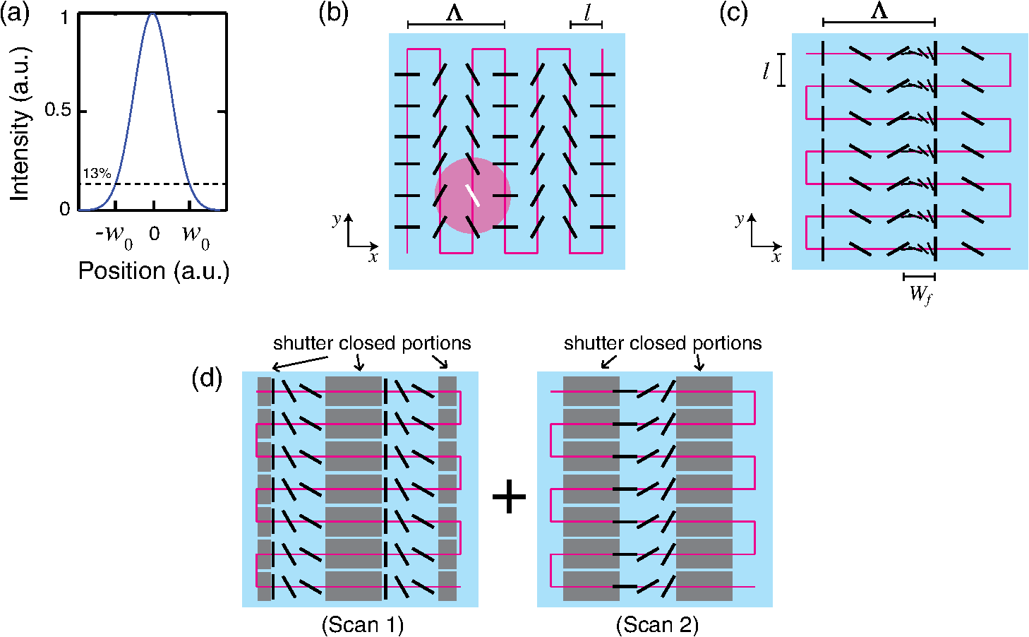 2.2.PG Materials and General ProcessingWe record the scanned polarization pattern within a layer of linear photopolymerizable polymer (LPP),21,22 which has been coated onto a glass substrate. After exposure, we coat one or more polymerizeable LC layers in order to realize the birefringent PG pattern. We note that as long as the thickness of each LC layer is small compared to the PG pitch, subsequent LC layers will have an alignment pattern practically identical to the layers underneath.23 A detailed protocol will be described in Sec. 3.4. Note that the essential principle is that the in-plane orientation angle of the LC nematic director at each position follows the fluence-weighted average of the multiple exposures of different linear polarizations at that position, as described more fully in Ref. 19. Therefore, throughout this work, we intentionally overlap neighboring scans in order to convert the discrete scan contours into continuous LC orientation profiles. However, this is limited by the fact that the local net polarization purity, i.e., the local net degree of linear polarization (DOLP), degrades if the overlap becomes too large and results in weak LPP anchoring strength and poor LC alignment. This DOLP is not identical to the typical DOLP of a single polarization state. It is the time-averaged net degree of linear polarization at each position and is derived in Ref. 19. 2.3.PG Figures of MeritWhile the quality of a PG can be quantified using many possible performance metrics, here we will use polarizing optical micrographs and transmission measurements. We define the diffraction efficiency as , where is the power in the ’th far-field diffraction order, and is the total power in the output hemisphere (measured as the transmission through a reference substrate). We, therefore, define haze, i.e., the fraction of light scattered outside the diffraction orders, as . Additionally, we define the polarization contrast as . For all our optical measurements, we input a circularly polarized probe laser, which is selected to maximize diffraction in the order and minimize diffraction into the order. Because we find that essentially every type of deviation from the ideal PG anisotropy, in simulation and/or experiment, causes some detectable degradation in efficiency, haze, or polarization contrast, we will use these metrics as the primary figures of merit in this work. 3.Optimizing Scan PathThe optical axis profile of a PG is illustrated in Fig. 1(b), where the characteristic dimension is its period (usually in the range of micrometers to millimeters). Since we are interested in PGs with clear aperture on the scale of centimeters, the small spot [Fig. 1(a)] must be scanned along a contour within the three dimensions of the parameters space (i.e., two spatial and one orientational). Since the scanning speed and extent of each dimension are, in general, not the same, it is not trivial to determine the optimal contour, and if poorly chosen, the scan times may be unfeasibly long. Based on the symmetry of the PG profile, we identify three candidate scan paths for study, illustrated in Figs. 1(b)–1(d). Each is a series of parallel lines spaced a distance apart, which is necessarily constrained by . 3.1.Perpendicular ScanThe first path comprises scan lines that are perpendicular to the grating vector,19 shown in Fig. 1(b). The difference in orientation between adjacent lines is rad. Although this pattern consists of a discrete number of polarization angles, the LC orientation angle smoothly varies from one scan line to the next due to the averaging properties of the LPP and LC materials. Because is constant for each scan along the dimension, the beam scanning speed is limited principally by the translation stages. The total time of each scan line has two parts: the time required to traverse a single line of height and the time required to reverse direction and begin the next scan line, such that . If we assume the speed within each line is approximately constant, then . The time to reverse direction depends additionally on both the maximum acceleration and jerk time (i.e., the maximum time required to change acceleration), such that . In our translation stages, and . Notice that the speed affects these times in opposite ways: faster speeds decrease but increase , and vice versa. To find the optimal scan speed needed to minimize time , we find and solve for . This leads to an optimal speed of . In our experience, this leads to typical speeds in the range from 10 to depending on . 3.2.Parallel ScanThe second path comprises scan lines that are parallel to the grating vector, as shown in Fig. 1(c), where changes continuously within each line. A similar approach was used in Ref. 20, where a line-shaped beam was scanned while the polarization continuously varied. In these cases, the primary limitation is the speed of polarization cycling (in degrees/second) or, alternatively, the polarization modulation frequency (in Hertz). One option is a rotating half-waveplate,20 but this is limited to a few hundred deg/second at best. As an alternative, the polarization modulator configuration (i.e., including a Pockels cell) we employ allows for rapid and continuous change of polarization orientation (up to ). However, its range is strictly limited to . This requires flipping the polarization modulator’s setting within every PG period from one extreme to the other (e.g., from to ), thereby quickly traversing through all the polarization states between those extremes. We call the LPP region exposed by these incorrect polarizations the flip region. The flip region is highly undesirable, as the incorrect polarizations result in a nonlinear orientation profile and/or degrade the LPP anchoring strength. The width of the flip region relative to the period can be estimated as , where is the polarization modulation frequency. In our system, the maximum rate the polarization can be modulated consistently is 5 kHz. The scan speed can, therefore, be found as . 3.3.Shuttered Parallel ScanThe third path is identical to the parallel scan, except that the flip region is eliminated. To remove the flip region, the path is scanned twice [Fig. 1(d)], with the flip region on each scan adjusted to opposite sides of each period, and a shutter is used to block the laser illumination during each the flip region. The downside is that is now limited by the shutter modulation frequency . In our implementation, the speed may be found as . 3.4.Experimental ComparisonWe fabricated PGs using each of the three scan patterns on different regions of the same substrate. All three scans had period , line spacing , a recording beam with diameter , and a speed and power resulting in a spatially averaged fluence of . The parallel scan had , and for the shuttered parallel scan, . The LPP/LC processing was as follows, which is optimized to achieve a half-wave retardation for 633 nm wavelength. The photoalignment material ROP-108 (Rolic) was coated (1500 rpm, 30 s) on clean glass substrates, followed by baking on a hotplate (1 min, 115 deg). After exposing this LPP, a 3:1 solution of the polymerizeable LC solution RMS03-001C (Merck) and propylene glycol monomethyl ether acetate was coated (1200 rpm, 75 s). The LC layer was dried and cured with blanket UV within a dry nitrogen environment (1 min, 365 nm at ). Finally, another LC layer was coated using the same processing conditions as the first LC layer. Polarizing optical micrographs of each result are shown in Fig. 2. We observe that the perpendicular scan manifests the most regular and smooth texture, implying the best alignment. The parallel scan result includes many LC disclination defects, resulting from poor LPP anchoring strength caused by the polarizing flipping. The shuttered parallel scan appears to be nearly free from these defects and shows almost the same quality as the perpendicular scan. Fig. 2Polarizing optical micrographs of the PGs written with three scan paths: (a) perpendicular scan, (b) parallel scan, and (c) shuttered parallel scan. All scans had , , , and a speed and power resulting in a spatially averaged fluence of . Different shades correspond to different alignment orientations.19 Note that each period includes two dark fringes because the intensity observed in this view is the same for and .  It is now important to compare the scan times of these two scan paths. As a hypothetical case, consider a area with and : the perpendicular scan would take (at ), while the shuttered parallel scan would take over 1.5 years (since )! Clearly, only the perpendicular scan is feasible. Even the regular parallel scan would take over one day (at ). We conclude that while the shuttered parallel scan may be usable in some situations, the perpendicular scan pattern is much more practical and does not appear to have any disadvantages. We use the perpendicular scan pattern for the remainder of this paper. 4.Optimizing Scan ParametersOnce the scan path type is chosen, there are four parameters that must be chosen to record any particular PG: , , , and the spatially averaged fluence . Since these four scan parameters have a wide range of feasible values, the design space is very large. The purpose of this section is to describe and employ an efficient and reliable method for selecting optimal parameters for the creation of PGs with high . 4.1.Parameter Space NormalizationWe begin with the assumption that the LC alignment at any point is governed solely by the exposure of the LPP directly beneath it. While it is clearly very simplistic and neglects the influence of the LC itself and hence, will not be valid when the grating period approaches the scale of the LC thickness, it enables the development of a valid first-order predictive model. 4.1.1.Normalized line spacing and beam sizeWith this assumption, we can reduce the dimensions of the parameter space by normalizing the beam size and line spacing to the period. We define the normalized line spacing and the normalized beam size as follows: An additional dependent parameter will also be helpful for defining, the beam overlap . It may be helpful to illustrate the meaning of these parameters with some examples: means that the line spacing is one tenth of the period and that there are 10 scan lines per period; means that the beam diameter is one tenth the size of the period; and means that the beam size and line spacing are the same size; hence, minimal overlap occurs but the entire pattern is still exposed. Note that the illustrated scan in Fig. 1(b) has and for the illustrated intensity profile in Fig. 1(a). The line spacing linearly affects the scan time, which is particularly important for PGs with large areas or/and small . For example, if scanning a single line takes 0.5 s and the PG area is , then for and , i.e., , the total scan time will be 42 h. Such long scan times are undesirable for a number of reasons: (1) it severely limits throughput; (2) there is greater risk of uncontrollable external forces affecting the scan (e.g., vibrations, air currents, laser fluctuations); (3) there is greater susceptibility to dust particles settling on the LPP; and (4) the LPP may undergo degradation after such a long time (e.g., due to water vapor or oxygen). Therefore, an optimum set of scan parameters will have an as large as possible without degrading PG quality. 4.1.2.Spatially averaged fluenceWhen the spot with a Gaussian intensity profile is scanned in neighboring lines, the local fluence will have at least some local variation, especially when is not large. This is important since good LC alignment is possible only if the fluence is higher than a threshold.19 However, if the fluence is too high, then the LPP may saturate, resulting in unexpected LC alignment. Therefore, the fluence should be as high as possible everywhere without saturating the LPP. However, we do not choose directly, but instead choose the spatially averaged fluence , which is related to via . Experimentally, we find that a spatially averaged fluence of results in local fluence variations that are within the desired window of fluence values for a wide range of scan parameters, and this value is used for the remainder of this paper. Last, we note that, in practice, is controlled by setting the speed of the scan and total beam power to satisfy the following equation: 4.2.Scan Parameter AssessmentWe assess any given scan parameter combination (, , and ) by examining the resulting PG first-order efficiency, in either simulation or experiment. The first step is to use the mathematical formalism given in Ref. 19 to predict the LC response, which is characterized by the orientation angle and alignment confidence . We set since the LPP we use here aligns parallel to the direction of the exposing linear polarization; furthermore, note that a zero pretilt is always assumed. The alignment confidence is bounded between 0 and 1 and represents our confidence that the LC will align along . It is calculated from and , as described in Ref. 19. Physically, variations in may correlate with variations in the alignment strength of LPP, out-of-plane tilt, LC order parameter, and LC scattering. However, in this study, we are interested only in scan patterns that result in as close to unity as possible, since this correlates to strong, in-plane anchoring without haze. After obtaining19 the vector field , the PG diffraction behavior can be simulated by assuming the phase profile of PG is twice the LC orientation angle: . This follows from theory regarding the geometric phase (Pancharatnam-Berry phase).24 With , the appropriate near-to-far-field transformation3 is applied to obtain the far-field diffraction orders . The first-order diffraction efficiency is a particularly useful scalar number with which to assess a scan parameter set. As an example of a poorly performing parameter set, consider and . The intensity cross-section for all scan lines impacting a single period is given in Fig. 3(a). This sparse scan leads to the spatially varying fluence, , shown in Fig. 3(b) and the shown in Fig. 3(c). The associated and are shown in Figs. 3(d) and 3(e). Finally, the diffraction efficiency for all orders is shown in Fig. 3(f). Now we can judge the effectiveness of this scan parameter combination. First, note that the diffraction efficiency is only 84%, and leakage may be seen in the other orders. Second, the low alignment confidence in portions of Fig. 3(d) implies that this region may have substantial disorder in the LC, which is likely to dramatically increase haze and reduce the diffraction efficiency even further than predicted in Fig. 3(f). Fig. 3Simulation of scan parameters leading to poor diffraction behavior, with , , and : (a) intensity cross-section for each scan line affecting a single period; (b) net fluence; (c) net ; (d) alignment confidence ; (e) resulting phase . (f) Diffraction efficiencies, found by applying the near-to-far-field transformation (NTFFT) on (e).  Conversely, a much better parameter set is shown in Fig. 4, with and . With this larger beam size and smaller line spacing [Fig. 4(a)], much more averaging of the orientation profile takes place. This results in a virtually constant local fluence [Fig. 4(b)], [Fig. 4(c)], and [Fig. 4(d)]. Not surprisingly, this leads to a very linear phase profile [Fig. 4(e)], and high single-order diffraction efficiency [Fig. 4(f)], predicted as . Since is close to unity everywhere, we choose to trust the calculated , and we judge this as an excellent set of scan parameters. Fig. 4Simulation of scan parameters leading to excellent diffraction behavior, with , , and : (a) intensity cross-section for each scan line affecting a single period; (b) net fluence; (c) net ; (d) alignment confidence ; (e) resulting phase . (f) Diffraction efficiencies, found by applying NTFFT on (e). 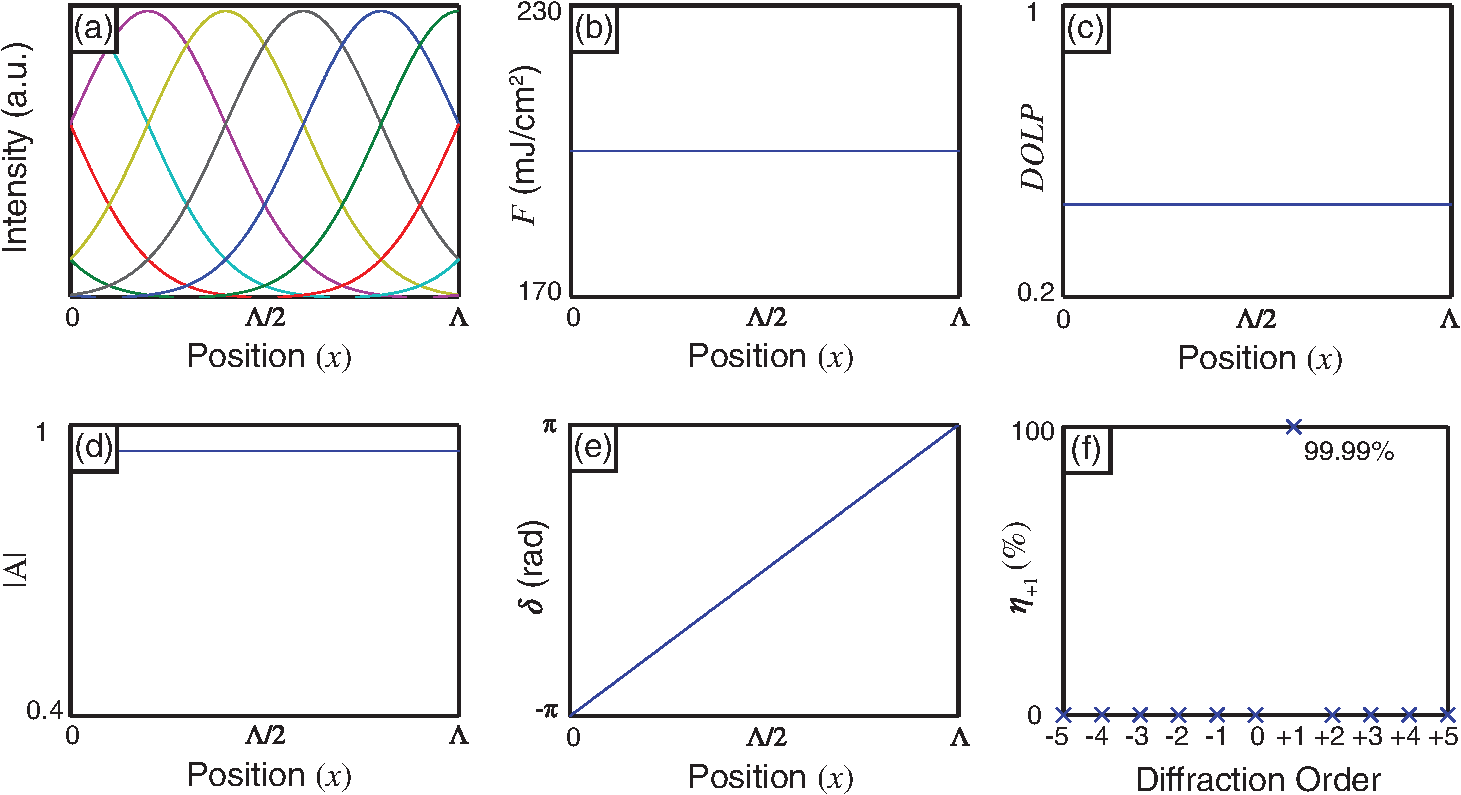 4.3.Parameter Space AnalysisTo map the parameter space, we applied this analysis to a range of and . In Fig. 5, we show minimum value of the predicted , and in Fig. 6, we show the predicted first-order efficiency. With these two graphs, we can now offer an explanation as to the different degradation mechanisms in our direct-write PGs and identify optimal scanning parameters. Fig. 5Simulated minimum alignment confidence as a function of the normalized line spacing and normalized beam size . Note and were sampled in steps of 0.05 and 0.025, respectively, and for all cases. Values of noticeably lower than unity are associated with liquid crystal defects, incorrect retardation, and incorrect alignment orientation. 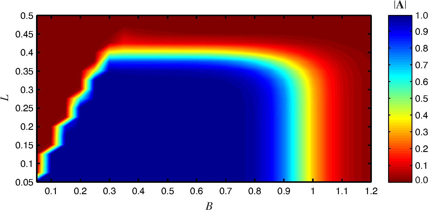 Fig. 6Simulated first-order diffraction efficiency as a function of the normalized line spacing and normalized beam size . Note and were sampled in steps of 0.05 and 0.025, respectively, and for all cases. For this simulation alone, we furthermore assumed .  Recall that whenever is noticeably lower than unity, it indicates that at least some part of every period has poor alignment. This may occur if the local fluence or/and DOLP are too low. Consider the former (fluence): since we have fixed , the only way some positions receive a too-low fluence is when the beam size is small relative to the line spacing, i.e., when is low. In Fig. 5, this begins to occur at the left portion of the graph, where . Now consider the latter (DOLP): as increases, the polarization difference between neighboring scan lines increases. Assuming remains constant, this results in a decreased DOLP for positions within a period. In Fig. 5, this occurs at the upper portion of the graph, beginning around . Finally, note that if , which means that the beam size is larger than the period, then the DOLP will be low, regardless of . In Fig. 5, this occurs at the right portion of the graph, beginning around . It is important to note that even with high alignment confidence, may still be low because the recorded may not be linear enough. This results in parameters that lead to a nonlinear . To isolate this, we can simulate the phase pattern resulting from each point in the parameter space while assuming that . This is shown in the graph of Fig. 6, within which we observe these trends: diffraction efficiency is better for larger and/or lower . Our understanding of this is that a larger results in a higher and a lower results in more scan lines per period, both of which result in a more linear profile. 4.4.Optimal Scan ParametersOur prime interest are those scan parameters that result in for which we have high alignment confidence (i.e., ). This subset of the parameter space can be approximated as a triangle, as shown in Fig. 7, by combining Figs. 5 and 6. This is the range where and . Fig. 7Predicted optimal parameter space for direct-writing PGs with high efficiency. Parameters inside the white triangular region are predicted to have high efficiency. Since scans with larger result in a shorter scan time, we identify the point that offers minimum scan time while preserving a predicted efficiency of . Since scans with parameters furthest away from the edges of the optimal parameter space will be the most robust with regard to small variations in scan parameters, we identify the point that offers maximum alignment quality while preserving a predicted efficiency of . 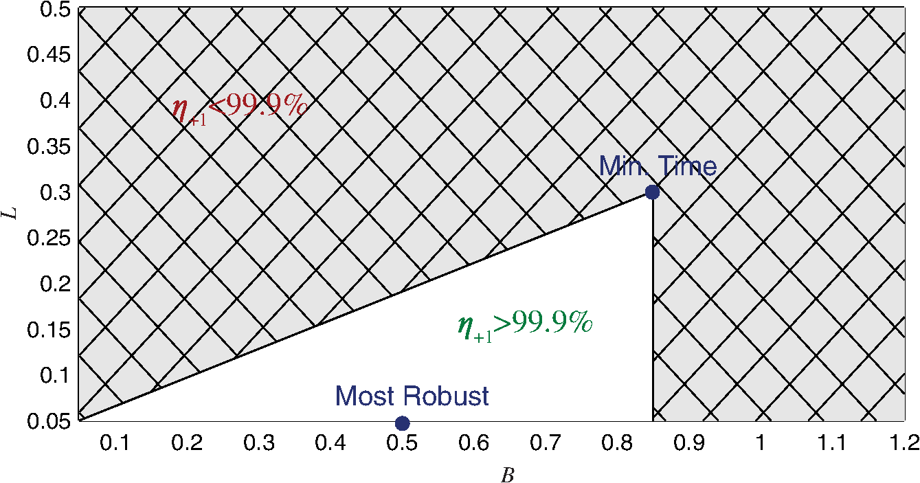 If minimizing the total scan time is the primary concern, then choosing and is ideal. If maximizing alignment quality is the primary concern (i.e., reaching for the highest possible ), then choosing and could be considered ideal. This parameter set is robust with regard to small variations in scan parameters and, so, may also be particularly useful when the beam size cannot be controlled precisely or when attempting small . 5.Error AnalysisIn a real direct-write system, errors not accounted for in the above analysis will appear and may influence the resulting PG behavior. In our experience, the primary error modes are in the beam power, beam size, and beam polarization angle. Errors in beam power and beam size are easily expressed as percentage deviations from the nominal values. Polarization error is more complex: for systems that use a variable retarder, such as ours, the actual polarization angle will be for some nominal polarization angle . Because the polarization of a PG pattern is periodic, the resulting polarization error varies as a function of position. To get around this, we define the polarization error as the maximum normalized difference between the nominal and actual polarization . As a representative example, we examine the error sensitivity around , , and , chosen to match the experimental results in the next section. At the nominal values, and . To identify the minimum significant error for each parameter, we assume that any degradation exceeding or is significant. The resulting error sensitivities are summarized in Table 1. Table 1Minimum significant error leading to degradation exceeding η+1≥99.5% or |A|≤0.9.
These results indicate that polarization error is the most sensitive and, thus, the most important to mitigate through calibration and persistent monitoring. Errors in beam power or beam size that cause significant impact on the PG quality are unlikely to occur, even in a system that is calibrated only moderately well, since the sensitivity to either is very low, at least at this and parameter set. 6.Experimental ResultsTo test the predictions of the parameter space optimization, we fabricated nine PGs with different parameters and measured the resulting . All PGs were written on the same substrate, with , , and an area of each. The LPP/LC coating protocol was the same as in Sec. 3.4, with the additional final step of laminating antireflection glass on both sides. The nine PGs ( through ) were recorded with parameters along the grid defined by and , shown overlaid with the optimal parameter space in Fig. 8. Based on the analysis of Sec. 4.4, we expect cases , , , , and to result in high-quality PGs. Although and lie just outside the simplified optimal parameter space of Fig. 7, their predicted is still . Fig. 8The nine parameter sets used for the experimental fabrication of PGs, overlaid on the optimal parameter space identified in Fig. 7. Also shown are the measured for each case. 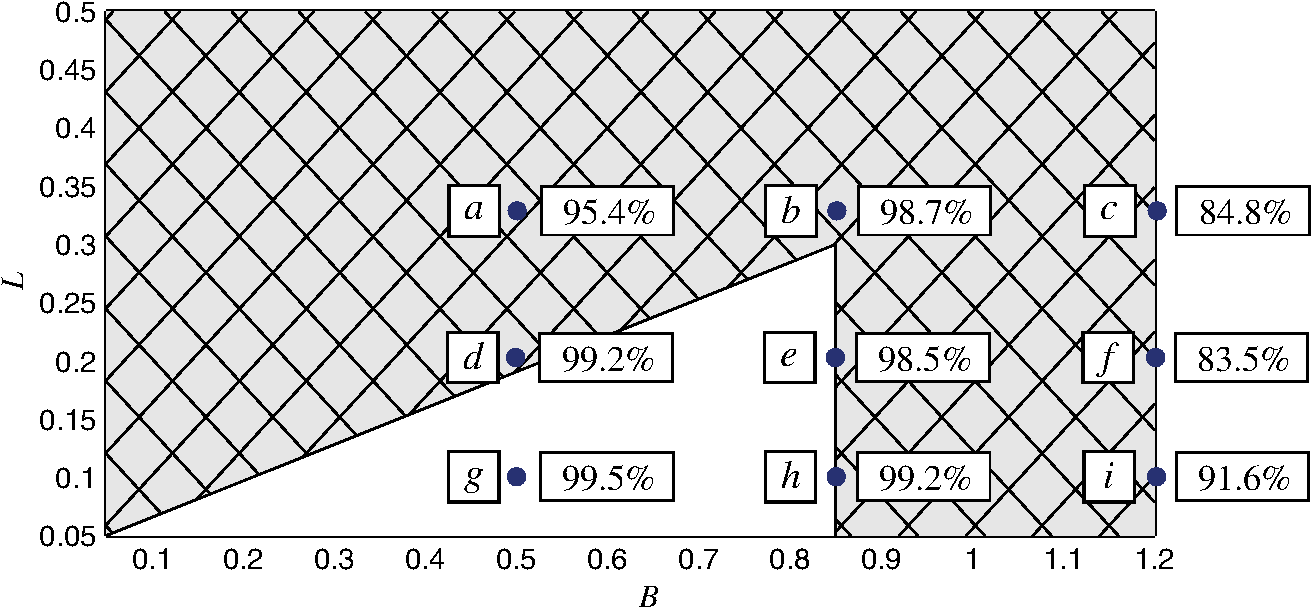 Polarizing optical micrographs of each result are shown in Fig. 9. There are three notable lessons: (1) the PGs with parameters from the right side of the parameter space (, , and , corresponding to ) show many LC defects; (2) the case PG is visibly nonlinear and uneven; and (3) the remaining cases (, , , , and ) show no apparent alignment problems and are almost indistinguishable by eye. Fig. 9Polarizing optical micrographs of the PGs with parameters shown in Fig. 8 and Table 2, between crossed polarizers. Different shades correspond to different alignment orientations.19 For all, ; note that each period includes two dark fringes because the intensity observed in this view is the same for and . The normalized beam size (B) is the ratio of the beam size to the grating pitch; the normalized line spacing (L) is the ratio of the line spacing to grating pitch: (a) large L and small B, (b) large L and medium B, (c) large L and large B, (d) medium L and small B, (e) medium L and medium B, (f) medium L and large B, (g) small L and small B, (h) small L and medium B, (i) small L and large B. 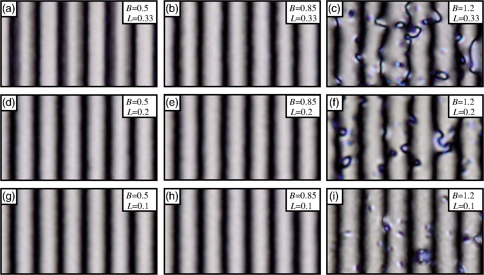 We furthermore characterized the diffraction behavior of each PG using a circularly polarized 633 nm (HeNe) laser. The diffraction efficiencies, haze, and polarization contrast for each parameter set are listed in Table 2, and (alone) is shown for each in Fig. 8. As expected, the PG with parameters showed the highest efficiency (), and its two nearest neighbors and were the second best (). All of these had low haze () and high polarization contrasts (). Table 2Measured polarization grating diffraction behavior of the cases identified in Fig. 9. Measurement error on all diffraction efficiencies is ±0.05%.
7.DiscussionAll of the experimental results support the overall predictions of Sec. 4.4, and especially the optimal parameter space identified in Fig. 7. Notably, the PG with the highest experimental efficiency had parameters () closest to the Max. Quality point identified within the simulation study. While none of the experimental patterns showed , the best result of is comparable to the best quality PGs recorded via other methods.3,4,14,25 A number of practical issues may be responsible for the lower-than-ideal efficiency, including incorrect retardation, reflections between the LC/glass interface, and errors in the polarization calibration of the system. We expect that the use of substrates with more advanced coatings, additional optimization of LPP/LC processing steps, and further system calibration, should lead to even higher efficiencies than reported here. One topic we have been silent on until now is the minimum achievable with good alignment and high diffraction. It should be obvious that this will be limited, in part, by the beam diameter (), mostly controlled by the laser itself and the objective lens. For a fixed beam diameter, the minimum corresponds to the maximum , as Eq. (2) teaches. Furthermore, the prediction of Fig. 7 is that is the largest value that may be expected to produce high efficiency and good alignment. Since our system has a minimum beam diameter , this predicts that the minimum we can record should be as low as , which has thus far been confirmed by our preliminary experiments. In Sec. 6, we selected several parameters with because, in this case, is an integer. In our experience, we find that when is not an integer, lower-quality PGs result, usually with diffraction along orders below , due to the fact that a noninteger means that the absolute polarization of each scan line repeats with a periodicity larger than . Our simulation (Sec. 4) is clearly limited by our assumptions, and it is true that we may not be able to fully understand the detailed phenomena of direct-write PGs until a more advanced simulation is developed. In particular, we anticipate that the analytical tools discussed here may breakdown under these conditions: for small (e.g., ), for large fluence (e.g., ), and for writing beams with non-Gaussian intensity profiles. Note that the optimization approach described here for PGs can be almost directly applied to many other patterns suitable for direct-writing, including -plates,26,27 forked PGs,28 and even arbitrary patterns.29 Finally, while the elements we studied here are all fixed polymer LC layers on single substrates, we anticipate similar behaviors on switchable PGs formed with two substrates,4,7 or even PGs formed with different materials30 altogether. 8.ConclusionsIn this study, we examined the parameter space for direct-write PGs in both simulation and experiment. We found that the perpendicular scan path is optimal since it offers the shortest scan times when the translation stages are significantly faster than the polarization modulator. We also mapped out the parameter space in simulation, which led to the prediction that PGs formed with the parameters and should have excellent diffraction properties for grating periods within . By fabricating several PGs within and around these limits, we confirmed that experimental PGs can be made with high efficiency (99.5%) and that the general trends of the first-order model appear valid. Finally, we simulated the sensitivity of PG behavior to errors in beam power, beam size, and polarization, and identified that our system is most sensitive to polarization errors of the writing beam. We have shown that it is possible to create direct-write PGs with diffraction behavior equivalent to the best PGs formed by holographic lithography. This is important because the direct-write lithography approach enables larger clear apertures, much easier adjustment of , multiple gratings on one substrate, and more consistent results. AcknowledgmentsThe authors gratefully acknowledge the support of the National Science Foundation (NSF PECASE grant ECCS-0955127). ReferencesL. NikolovaT. Todorov,
“Diffraction efficiency and selectivity of polarization holographic recording,”
Opt. Acta, 31
(5), 579
–588
(2010). http://dx.doi.org/10.1080/713821547 OPACAT 0030-3909 Google Scholar
G. Crawfordet al.,
“Liquid-crystal diffraction gratings using polarization holography alignment techniques,”
J. Appl. Phys., 98 123102
(2005). http://dx.doi.org/10.1063/1.2146075 JAPIAU 0021-8979 Google Scholar
M. J. Escutiet al.,
“Simplified spectropolarimetry using reactive mesogen polarization gratings,”
Proc. SPIE, 6302 630207
(2006). http://dx.doi.org/10.1117/12.681447 PSISDG 0277-786X Google Scholar
J. Kimet al.,
“Wide-angle, nonmechanical beam steering with high throughput utilizing polarization gratings,”
Appl. Opt., 50
(17), 2636
–2639
(2011). http://dx.doi.org/10.1364/AO.50.002636 APOPAI 0003-6935 Google Scholar
C. Ohet al.,
“High-throughput continuous beam steering using rotating polarization gratings,”
IEEE Photonics Technol. Lett., 22
(4), 200
–202
(2010). http://dx.doi.org/10.1109/LPT.2009.2037155 IPTLEL 1041-1135 Google Scholar
J. Kimet al.,
“Efficient and monolithic polarization conversion system based on a polarization grating,”
Appl. Opt., 51
(20), 4852
–4857
(2012). http://dx.doi.org/10.1364/AO.51.004852 APOPAI 0003-6935 Google Scholar
R. K. Komanduriet al.,
“Polarization-independent modulation for projection displays using small-period LC polarization gratings,”
J. Soc. Inf. Disp., 15
(8), 589
–594
(2007). http://dx.doi.org/10.1889/1.2770860 JSIDE8 0734-1768 Google Scholar
R. K. KomanduriC. OhM. J. Escuti,
“Polarization independent projection systems using thin film polymer polarization gratings and standard liquid crystal microdisplays,”
in SID Symp. Digest,
487
–490
(2009). Google Scholar
M. W. Kudenovet al.,
“White-light channeled imaging polarimeter using broadband polarization gratings,”
Appl. Opt., 50
(15), 2283
–2293
(2011). http://dx.doi.org/10.1364/AO.50.002283 APOPAI 0003-6935 Google Scholar
C. Packhamet al.,
“Polarization gratings: a novel polarimetric component for astronomical instruments,”
Publ. Astron. Soc. Pac., 122
(898), 1471
–1482
(2010). http://dx.doi.org/10.1086/657904 PASPAU 0004-6280 Google Scholar
G. Cincotti,
“Polarization gratings: design and applications,”
IEEE J. Quantum Electron., 39
(12), 1645
–1652
(2003). http://dx.doi.org/10.1109/JQE.2003.819526 IEJQA7 0018-9197 Google Scholar
G. CipparroneA. MazzullaL. Blinov,
“Permanent polarization gratings in photosensitive Langmuir-Blodgett films for polarimetric applications,”
J. Opt. Soc. Am. B, 19
(5), 1157
–1161
(2002). http://dx.doi.org/10.1364/JOSAB.19.001157 JOBPDE 0740-3224 Google Scholar
M. W. Kudenovet al.,
“Spatial heterodyne interferometry with polarization gratings,”
Opt. Lett., 37
(21), 4413
–4415
(2012). http://dx.doi.org/10.1364/OL.37.004413 OPLEDP 0146-9592 Google Scholar
E. Nicolescuet al.,
“Polarization-insensitive variable optical attenuator and wavelength blocker using liquid crystal polarization gratings,”
J. Lightwave Technol., 28
(21), 3121
–3127
(2010). http://dx.doi.org/10.1109/JLT.2010.2078487 JLTEDG 0733-8724 Google Scholar
B. Goekceet al.,
“Femtosecond pulse shaping using the geometric phase,”
Opt. Lett., 39
(6), 1521
–1524
(2014). http://dx.doi.org/10.1364/OL.39.001521 OPLEDP 0146-9592 Google Scholar
S. Nersisyanet al.,
“Optical axis gratings in liquid crystals and their use for polarization insensitive optical switching,”
J. Nonlinear Opt. Phys., 18
(1), 1
–47
(2009). http://dx.doi.org/10.1142/S0218863509004555 JNOMFV 0218-8635 Google Scholar
J. KimR. K. KomanduriM. J. Escuti,
“A compact holographic recording setup for tuning pitch using polarizing prisms,”
Proc. SPIE, 8281 82810R
(2012). http://dx.doi.org/10.1117/12.913952 PSISDG 0277-786X Google Scholar
M. N. Miskiewiczet al.,
“Progress on large-area polarization grating fabrication,”
Proc. SPIE, 8395 83950G
(2012). http://dx.doi.org/10.1117/12.921572 PSISDG 0277-786X Google Scholar
M. N. MiskiewiczM. J. Escuti,
“Direct-writing of complex liquid crystal patterns,”
Opt. Express, 22
(10), 12691
–12706
(2014). http://dx.doi.org/10.1364/OE.22.012691 OPEXFF 1094-4087 Google Scholar
H. OnoT. WadaN. Kawatsuki,
“Polarization imaging screen using vector gratings fabricated by photocrosslinkable polymer liquid crystals,”
Jpn. J. Appl. Phys., 51
(3), 030202
(2012). http://dx.doi.org/10.1143/JJAP.51.030202 JJAPA5 0021-4922 Google Scholar
M. Schadtet al.,
“Surface-induced parallel alignment of liquid-crystals by linearly polymerized photopolymers,”
Jpn. J. Appl. Phys., 31
(Part 1, No. 7), 2155
–2164
(1992). http://dx.doi.org/10.1143/JJAP.31.2155 JJAPA5 0021-4922 Google Scholar
O. YaroshchukY. Reznikov,
“Photoalignment of liquid crystals: basics and current trends,”
J. Mater. Chem., 22
(2), 286
–300
(2011). http://dx.doi.org/10.1039/c1jm13485j JMACEP 0959-9428 Google Scholar
C. OhM. J. Escuti,
“Achromatic diffraction from polarization gratings with high efficiency,”
Opt. Lett., 33
(20), 2287
–2289
(2008). http://dx.doi.org/10.1364/OL.33.002287 OPLEDP 0146-9592 Google Scholar
M. V. Berry,
“The adiabatic phase and pancharatnam phase for polarized-light,”
J. Mod. Opt., 34
(11), 1401
–1407
(1987). http://dx.doi.org/10.1080/09500348714551321 JMOPEW 0950-0340 Google Scholar
C. ProvenzanoP. PagliusiG. Cipparrone,
“Highly efficient liquid crystal based diffraction grating induced by polarization holograms at the aligning surfaces,”
Appl. Phys. Lett., 89
(12), 121105
(2006). http://dx.doi.org/10.1063/1.2355456 APPLAB 0003-6951 Google Scholar
S. C. McEldowneyet al.,
“Creating vortex retarders using photoaligned liquid crystal polymers,”
Opt. Lett., 33
(2), 134
–136
(2008). http://dx.doi.org/10.1364/OL.33.000134 OPLEDP 0146-9592 Google Scholar
S. Nersisyanet al.,
“Fabrication of liquid crystal polymer axial waveplates for UV-IR wavelengths,”
Opt. Express, 17
(14), 11926
–11934
(2009). http://dx.doi.org/10.1364/OE.17.011926 OPEXFF 1094-4087 Google Scholar
Y. LiJ. KimM. J. Escuti,
“Orbital angular momentum generation and mode transformation with high efficiency using forked polarization gratings,”
Appl. Opt., 51
(34), 8236
–8245
(2012). http://dx.doi.org/10.1364/AO.51.008236 APOPAI 0003-6935 Google Scholar
F. Ottenet al.,
“The vector apodizing phase plate coronagraph: prototyping and new developments,”
Proc. SPIE, 9151 915161
(2014). http://dx.doi.org/10.1117/12.2054707 PSISDG 0277-786X Google Scholar
L. Nikolovaet al.,
“Polarization holographic gratings in side-chain azobenzene polyesters with linear and circular photoanisotropy,”
Appl. Opt., 35
(20), 3835
–3840
(1996). http://dx.doi.org/10.1364/AO.35.003835 APOPAI 0003-6935 Google Scholar
Biography |


