1.

Introduction

Range imaging (RI) refers to a family of technologies that aim to capture and extract the depth information of a scene. Formally, assuming that each point in a scene imaged by the sensor is characterized by a single depth value (the distance between the object and the camera), one can generate a depth map of a scene where pixel intensity corresponds to the distance between the camera and the imaged object. Depth information can be directly used for the visualization of the scene, as well as for target detection, robot navigation, and surface modeling. Today, several RI solutions are available in the market depending on the hardware requirements, the physical constraints, and the requested depth data quality and resolution. RI has been employed in numerous applications including remote sensing, gaming, security, search and rescue, and medical diagnostics.¹

RI systems can be broadly classified as active or passive, depending on the presence or absence of a user-controlled illumination source. Passive RI systems are designed such that depth information is extracted from a single or multiple images using properties of the scene or the imaging setup. Typical examples of passive RI including stereo, multiview imaging, and depth-from-focus methods that have been extensively used for extracting depth information, especially in indoor scenarios. On the other hand, active RI technologies adopt a user controlled illumination source for depth extracting. Laser-based active RI, also known as Light detection and ranging (LIDAR), is a well-known active RI technique that performs depth extraction based on the time-of-flight (ToF)² principle, i.e., by measuring the time it takes for a laser pulse to travel the distance from the source to the object and back to the sensor. Active RI technologies enjoy a broader range of applications, including night time and underwater imaging, due to the use of active illumination. Furthermore, active RI systems, especially the ones based on ToF depth estimation, achieve large measurement ranges and high quality depth estimation.

Currently, there are two categories of ToF camera architectures, namely, continuous-wavemodulation (CWM)³ and gated range imaging (GRI).^4–6 CWM-RI operates by illuminating the scene with an appropriately modulated light source and recording and extracting the depth by investigating the phase of the reflected light. In contrast with CWM, in GRI a series of pulses are emitted from the light source, and the sensor records the reflected pulses that correspond to a specific range of distances, by electronically controlling the on-off state of the gate. For each specific range, a depth profile is reconstructed according to the time interval in which the sensor registered the reflected pulses. To obtain a full depth map, multiple frames, whose number is proportional to the required depth resolution, have to be recorded. This technique is commonly referred to as the time slicing (TS) approach.

The range imaging capabilities of a GRI system are primarily dictated by the number of frames that the imaging sensor must capture in order to support the requested depth resolution. The temporal resolution in GRI architectures is therefore directly related to the depth resolution. A higher temporal resolution leads to a greater depth resolution that can provide a more detailed mapping of the scene and strengthen subsequent processing such as target detection. However, higher depth resolution comes at the cost of a larger number of frames, which implies slower acquisition process and restricts the capability of imaging dynamic scenes, or range imaging from a moving platform. Compactly, we define the sampling rate as the ratio between the acquired number of frames and the requested number of depth bins by $r=\#\mathrm{frames}/\#\mathrm{depthbins}$.

While traditional GRI requires $r=1$, which corresponds to the Nyquist rate sampling; in this work, we propose a novel architecture that can achieve the same depth resolution, at a much lower $r$. More specifically, we propose a novel GRI technique that is able to significantly reduce $r$ without sacrificing the quality of the depth map. This goal is achieved by exploiting the sparsity of the reflected laser pulses relative to the full resolution signals. Our proposed design, termed compressed gated range sensing (CGRS), shown in Fig. 1, employs a random gating mechanism for the temporal encoding of the reflected laser pulses. More specifically, the proposed architecture consists of a light source (laser), an electronic gating mechanism, and an imaging sensor. By dynamically varying the sampling pattern encoded by the mask during each frame, CGRS is able to achieve temporal multiplexing of the incoming light. Reconstruction of depth information from the multiplex signals is achieved by posing the problem in a compressed sensing (CS) framework and employing tools from the CS reconstruction theory. With respect to state-of-the-art approaches, the CGRS method:

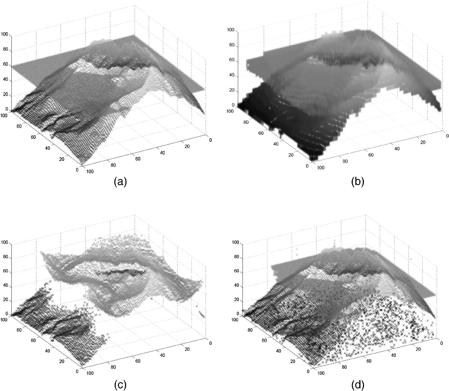
Fig. 1

A graphical overview of the proposed compressed gated range sensing (CGRS) architecture. At a specific time instance, a laser source transmits a pulse that propagates through some medium and is reflected back by objects in the scene, resulting in multiple reflected pulses, each one arriving at a different time instance (proportional to the traveled distance). An optical lens focuses the reflected pulses on a gating device that implements a coding mask for each pixel, corresponding to a random sampling of the reflected pulses. During each integration period (i.e., a single frame), the gating mask goes through a sequence of random pattern, temporally multiplexing the incoming light. As a consequence, each frame is associated with numerous mask states as shown in the projection matrix. Knowledge of the projection sequences and prior knowledge of signal behavior are exploited by CGRS to recover a high quality depth signal of the scene.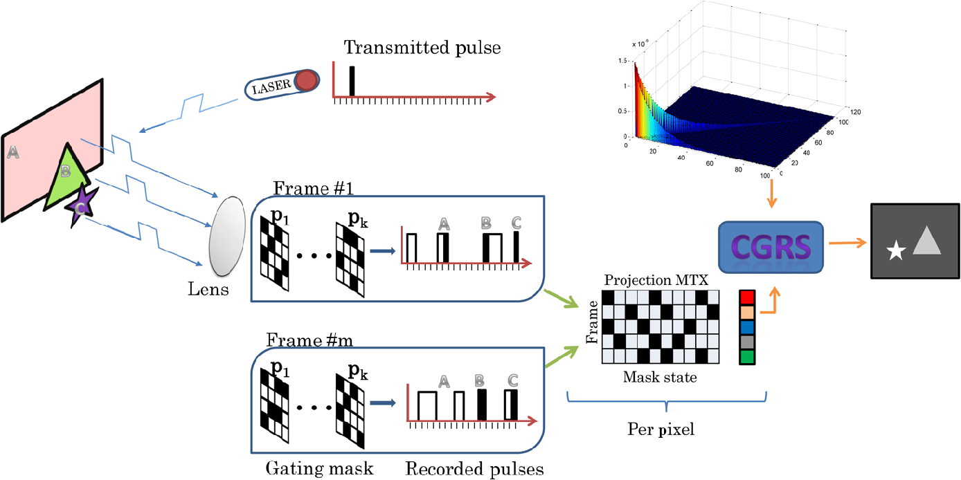

The rest of the paper is organized as follows. Section 2 provides an overview of current state-of-the-art in active RI, with a focus on GRI techniques. Section 3 presents an analysis on the characteristics of the depth signals, including their interaction with the various system components. Section 4 presents the proposed CGRS technology and discusses the characteristics of the individual components. To validate the merits of the proposed GRI scheme, Sec. 5 presents extensive experiments and comparisons with standard techniques that were carried out on data from a simulated system that was carefully designed to account for the numerous parameters that affect the behavior of a GRI setup. The paper concluding remarks are found in Sec. 6.

2.

Previous Work

Active RI systems such as LIDAR and structured light (SL) cameras make use of a light source in addition to the camera sensor to generate a depth map. In SL methods, a light projection system is responsible for illuminating the scene with a specific spatial pattern [typically in the near-infrared (NIR) part of the spectrum], while a camera sensor captures the reflected light.^7–9 In SL, the extraction of the depth map follows a similar approach as stereo imaging, albeit with known (or easily estimated) point correspondences that are identified by the distortion of the projected light patterns. Although when compared with stereo, SL avoids issues with correspondences, limitations of SL arise from specular reflections, strong dependence on illumination conditions, object motion, and the need for careful calibration.

ToF LIDAR approaches employ a ToF measurement process to quantify the scene’s depth profile by analyzing the time light takes to travel a specific distance. Two classes of ToF approaches have been developed, namely, GRI and CW modulation.¹⁰ In CW-ToF, a NIR projector, usually light-emitting diode based, projects a sinusoidal modulated light, while a complementary metal oxide semiconductor or a charge coupled device sensor measures the reflected light. To estimate depth, each sensor element must sample the reflected light four times at equal intervals for every period.¹¹ Using these measurements, one can estimate the phase, the offset, and the amplitude of the reflected light to extract a depth estimate. On the other hand, in GRI, the shutter of the camera sensor is carefully controlled in order to precisely manipulate the amount of reflected light that is captured at each frame. By limiting the exposure time, only laser pulses that have been reflected from objects at specific distance ranges are captured. As a consequence, to produce a detailed, high resolution depth map, multiple frames have to be captured.

The performance of a GRI system is determined by numerous parameters including the reflectivity of the scene, the atmospheric attenuation, and the effects of the gating process on the recorded signal. While some of these parameters can be reliably modeled, the interaction between the signal and the gating process is more complicated, but also allows for novel approaches in GRI. High precision sensor gain control is another technique for reducing the number of frames of classical GRI architectures. For example, one can employ a constant and a linearly increasing gain modulation by controlling the working voltage of the microchannel plates in order to achieve RI.¹² A similar approach¹³ was recently proposed where the authors investigated gain modulation for achieving depth map reconstruction from two frames by combining a narrow laser pulse generator with an exponentially modulated gain camera. The depth information of each pixel is calculated from the recorded value in two frames, one with constant gain and one with modulated gain. A significant issue related to this technology is that both methods require the ability to electronically control the gain of the sensor with a very high precision. Failure to accurately set the gain can lead to major depth estimation errors. Furthermore, the accuracy of the depth map varies with the target’s distance, which results in a nonuniform depth resolution. Finally, such technologies cannot handle multiple reflections due to the ambiguity that is introduced during the depth coding process.

TS is a benchmark method for depth extraction via GRI. According to this approach, the resolution of the depth map (number of depth bins) is directly proportional to the number of captured frames since each frame encodes depth information from a specific range only. For an overall depth range between $Z_{\min }$ and $Z_{\max }$, the depth range encoded in each bin corresponds to $Z_{\mathrm{bin}}=(Z_{\max }-Z_{\min })/K$, where $K$ is the number of captured frames. An object located at distance $z_k$ will produce a reflected pulse that will require $t_k=\frac{2z_k}{c}\sec$ to reach the sensor, where $c$ is the speed of light. Assuming that each measurement $m_n$, $n=1,\dots N$, encodes light from a specific depth range, the depth of a single object can be found by solving:

A significant shortcoming of the TS approach is the apparent waste of resources due to the acquisition of a large number of “empty frames”, that is, frames that do not capture any reflected pulse. Gate coding (GC) was recently proposed to address this issue.

GC is a novel approach in GRI that exploits the interaction between the profile of the pulse and the profile of the gate.^14–16 Formally, the intensity of a single pixel corresponding to an object at distance $z_k$, or equivalent time $t_k$, is given by the convolution of the laser pulse profile and the gate profile and is expressed as

GC assumes that both the laser and the gate exhibit rectangular intensity profiles, which implies that the resulting signal will have either a triangular or a trapezoidal depth intensity profile, depending of the relative duration of the pulse and the gate. As a consequence, the detector is capable of recording three distinct values, namely 0 for no signal, 1 for a plateau, and 0.5 for a rising or falling edge. The three values produce a constrained ternary code that is able to encode about $3^n-2^{n+1}+1$ valid combinations in $n$ images, thus offering super-resolved depth map estimation.

The proposed range imaging architecture can be considered as an example of flash LIDAR architecture.¹⁷ Flash LIADR technology relies on the transmission and receipt of a single laser pulse illuminating the scene. Depth estimation is achieved by exploiting the electric properties of avalanche photo diodes (APDs), which, when operating in Geiger mode, are able to magnify the signals generated by a small number of photons reaching the detector through an avalanche effect. A prominent example of this technology is the range imaging architectures developed by advanced scientific concepts (ASC) such as the ASC TigerEye.¹⁸ Although flash LIDAR architectures enjoy very intriguing properties, current designs based on APDs require specialized detectors that can increase the size and cost of the detector and have a negative effect on the spatial resolution. Furthermore, in-depth studies have shown that APD-based architectures are very sensitive to operating conditions, including range, laser power, and target occlusions.¹⁹

3.

Signal Modeling

The majority of systems presented in the GRI literature have been analyzed under ideal physical and operational conditions. However, a variety of noise sources, including sensor noise and optical turbulence, as well as the effects of various physical phenomena such as scattering and divergence of light beam, could be responsible for the breakdown of these systems under challenging yet realistic conditions. In this work, we consider a rigorous modeling of the numerous factors that affect the depth signals produced by GRI systems and incorporate this knowledge into the recovery process.

Formally, depth signals correspond to reflected laser pulses that reach the imaging sensor after propagating through the atmosphere. In GRI, the laser pulses are short in duration and transmitted during predefined periods. We assume that the reflected pulses are captured during distinct time intervals that result in a quantization of the depth map. The presence of multiple semi-transparent objects in the scene, including foliage and smoke, can lead to multiple reflected pulses being produced from a single transmitted pulse. Because of the very short duration of the pulses, one can model the depth signal, $\mathbf{s}(t)$, as a stream of $K$ weighted Dirac pulses taking place at specific time instances

In this equation, four factors are responsible for the power of the signals reaching the detector. More specifically, $Q$ is a factor encoding the efficiency of the system, $V(z)$ is the range-dependent geometry, $\beta (z)$ is the backscatter coefficient, and $T(z)$ is the atmospheric transmission term while $N$ encodes added Gaussian noise. The terms $V(z)$, $\beta (z)$, and $T(z)$ are all functions of the distance $z$, while the Gaussian noise incorporates all other nondistant-related noises sources. Next, we discuss the characteristics of each term.

In Eq. (5), the light source is modeled as a diverging source. The properties of this model are encoded in $V(z)$, which accounts for the attenuation of the power due to the geometric profile of the beam. Considering the path forward only, the divergence is given by

Light propagation through the atmosphere is primarily affected by three factors, namely absorption, scattering, and optical turbulence.²¹ While absorption and scattering are frequency-dependent phenomena that are manifested by a predictable attenuation of the optical waves, turbulence is a more complicated process that causes irradiance fluctuations. Absorption and scattering are often grouped together to a common term, the transmittance, described by Beer’s law as $T(z)=\exp (-a(\lambda )z)$, where $a(\lambda )$ is the extinction coefficient at distance $z$, combining the effects of both absorption and scattering. Since the recorded signal has undergone reflection, we have to take the atmospheric absorption into account twice. The value $\alpha =1/1000$ in meters is typically used for encoding clear and dry conditions. The atmospheric backscattering ${\beta }_{\pi }$ can be modeled as a constant density depending on the atmospheric conditions (weather and temperature). In clean conditions, we considered a value ${10}^{-7}$, while for wet conditions, a value in the range ${10}^{-5}$ can be used. Optical turbulence is modeled in our scheme as additive white Gaussian noise with a specific noise power. Finally, we assume that objects in the scene have a specific reflectivity $\le 1$ that may vary depending on the material.

While in theoretical models, the beginning and end of the laser pulse and the camera gate are modeled as instant operations requiring no transition time, in real-life conditions, this is no longer the case. To realistically model the behavior of the gate, we assume that the gate function can be expressed as the convolution of an ideal gate function, modeled by a rectangular function ${\mathbf{g}}_{\mathrm{ideal}}(t)=\mathrm{\Pi }(t+t_k)$, with a filtering function ${\mathbf{f}}_g(t)=e^{t/t_{\mathrm{gate}}}(t\ge 0)$ encoding the characteristics of the sampling process, that is $\mathbf{g}(t)={\mathbf{g}}_{\mathrm{ideal}}(t)*{\mathbf{f}}_g(t)$. Similarly, the laser pulse is modeled as the convolution of the ideal pulse ${\mathbf{x}}_{\mathrm{ideal}}(z)=\mathbf{s}(z)\mathcal{A}(z)\mathbf{d}(z)$ with a similar filter with parameter $t_{\mathrm{pulse}}$ giving $\mathbf{x}(t)={\mathbf{x}}_{\mathrm{ideal}}(t)*{\mathbf{f}}_p(t)$. As a consequence, the noise-free signal that reaches the sensor corresponds to the multiplication of the pulse function with the gate function defined before, that is $\mathbf{x}(t)={\mathbf{x}}_{\mathrm{ideal}}(t)\mathbf{g}(t)$. Considering the different noise sources and physical properties described above, the compound signal model is given by

To help visualize the effects on the previously discussed phenomena on the ideal depth signals, Fig. 2 showcases the progressive alteration of the ideal depth signal. In this figure, it is easy to understand that accounting for the different aspects of the system is critical in order to support the accurate and efficient recovery of the depth signals. Furthermore, these alterations are taken into account in the proposed CGRS via the introduction of a dictionary of prototypical examples, which we discuss in the next section.

Fig. 2

Graphical illustration of: (a) an ideal multiple reflection depth signal; (b) the signal with backscatter, turbulence, attenuation, and divergence; (c) the signal after interaction with the gate function. The horizontal axis encodes time and the vertical signal amplitude. Note that various effects, e.g., backscatter, are exaggerated compared with typical conditions for exposition.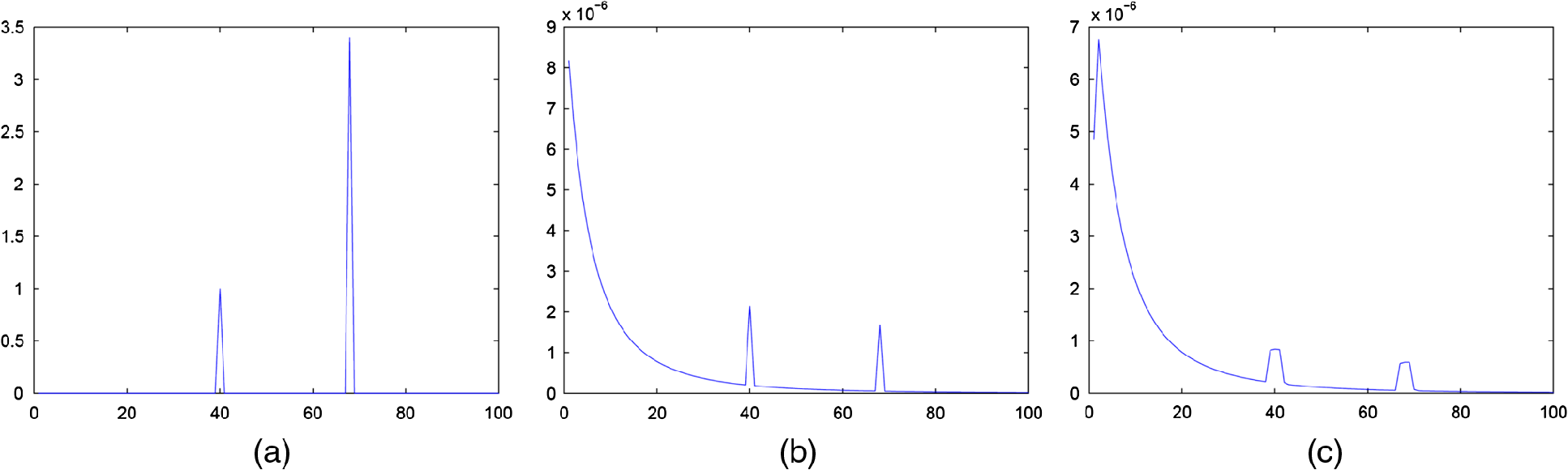

4.

Compressed Gated Range Sensing

The problem of extracting the true underlying signals from noisy and limited measurements has been extensively studied by the signal processing community. Formally, the number of measurements one is required to acquire is related to the bandwidth of the signal which, for a large class of signals, can be very high. The depth signals considered in GRI fall under this category, and thus require a large number of measurements, i.e., frames, for the accurate estimation of distances. Fortunately, the special structure of these signals can provide a significant boost in the recovery process.

Compressed sensing (CS) is a novel approach in signal representation and sampling that was introduced by Donoho²² and by Candes et al.²³ The main concept underpinning CS is that a signal can be recovered from a small number of random measurements that can be far below the Nyquist–Shannon limit. The key CS assumptions are that (a) the signal itself is sparse or that it can be sparsely represented in an appropriate dictionary, and that (b) enough random measurements are taken. Formally, a signal $\mathbf{s}\in {\mathbb{R}}^n$ is called $k$-sparse if ${\Vert \mathbf{s}\Vert }_0<k$, where the zero norm ${\Vert ·\Vert }_0$ counts the nonzero signal elements. This signal can be reliably recovered from a low-dimensional representation $\mathbf{y}=\mathbf{\Psi }s\in {\mathbb{R}}^m$, where $m\ll n$ by solving an $l_0$ constrained minimization problem given by

When the measurements are affected by noise or when an approximate solution is needed, one can solve the following approximate minimization problem:

Although CS has been developed fairly recently, it has already found many applications in imaging systems ranging from single pixel cameras²⁴ to CS-based magnetic resonance imaging,²⁵ and CS-based radar systems.²⁶ In all these applications, a dramatic increase in resolution or reduction in imaging time has been reported. CS-based imaging has also been investigated in the context of range imaging. The compressive depth acquisition camera (CoDAC)²⁷ is a prominent example of an active RI utilizing a single ToF-based sensor that capitalizes the properties of CS sampling and reconstruction. More specifically, the CoDAC designers propose to spatio-temporally modulate a light source and then sample the returning light by a single photon-counting photodetector. One of the most important attributes of this scheme is that the resolution of the depth map is matched with the resolution of the modulator, and thus providing a better spatial analysis than what is possible by the limited number of detectors.

The CoDAC RI system bears many similarities with the proposed GCRS architecture, most prominent being the use of CS for reducing the required sampling rate. While CGRS aims at increasing the depth resolution from a limited number of frames (temporal resolution increase), CoDAC aims at increasing the spatial resolution of the depth image. To achieve this, it requires a significant number of time samples that makes it impractical for dynamic scenes. Our proposed technique targets temporal resolution, which makes it more appropriate for time evolving scenes or for generating accurate depth maps from moving platform and vehicles. This work is an extension of an earlier version^28,29 and introduces numerous novel components, including the principled study of multiple pulse acquisition and decoding among others.

4.1.

Sensing Matrix

A critical component of the CGRS architecture is the random gating mechanism. Although one could consider deterministic sampling schemes, as is the case in TS and GC, the random sampling pattern is selected due to its fundamental properties with respect to recovery. Formally, to guarantee the stable recovery of the original signal $\mathbf{x}$, the $m\times n$ sensing matrix $\mathbf{\Psi }$ should satisfy the so-called restricted isometry property (RIP). A sensing matrix $\mathbf{\Psi }\in {\mathbb{R}}^{m\times n}$ satisfies the RIP with isometry constant $0\le \delta <1$ if for all $k$-sparse signals, $\mathbf{x}$, it holds that

Eq. (10)

$$(1-\delta ){\Vert \mathbf{x}\Vert }_2^2\le {\Vert \mathrm{\Psi }x\Vert }_2^2\le (1+\delta ){\Vert \mathbf{x}\Vert }_2^2.$$

Designing such a sensing matrix is proven to be a challenging task. However, it has been shown that matrices whose elements are randomly drawn from appropriate distributions satisfy the RIP with high probability. Examples of such distributions include normalized mean bounded variance Gaussian²² and Rademacher³⁰ distributions.

Although the construction of a sensing matrix via randomized methods has circumvented the need for explicit construction algorithms, many of the proposed sensing matrices are difficult to realize hardware-wise. In this work, the random measurements are generated by employing binary sparse matrices with a bounded number of nonzero elements per column.³¹ More specifically, the sampling matrix is constructed such that each element is drawn according to

Eq. (11)

$${\varphi }_{ij}=1/\sqrt{d}\{\begin{array}{ll}1& \text{with probability}\frac{\mathrm{dn}}{\mathrm{k}}\\ 0& \text{otherwise}\end{array}\mathrm{.}$$

The performance characteristics of this type of binary sampling matrices were recently explored,³² where it was shown that they satisfy the RIP. Obviously, their important advantage is that they approximate the performance of their dense counterparts, but at a significantly reduced computational and memory cost.

To help understand the benefits of our proposed random binary sampling scheme, Fig. 3 offers a visual exposition of applying the classical periodic and the novel random binary sensing approach when sampling sparse depth signals. In this figure, the (a) and (b) subfigures correspond to two depth signals, corresponding to objects at different distances. The repetition of the signals is a common approach in GRI aiming at increasing the power of the captured signals. The top row in each subfigure indicates the returning laser pulse, after it has been reflected by the object while the second and fourth rows present the periodic and random gating functions, respectively. We observe that periodic sampling follows a canonical pattern of leaving the gate open, while the proposed random gating opens and closes the gate multiple times within the integration time. The third and firth rows illustrate the captured signals. In the case of the left subfigure, the target happens to be at a range where both the periodic and the random gating functions are able to record energy from the returning laser pulse. However, in the right subfigure, we observe that the misalignment between the returning pulse and the periodic gating results in an all-zero captured signal. On the other hand, the proposed random sampling is still able to record a valuable signal. As a result, the recorded energy by the random gating method can be used to infer the location of the target and to estimate its distance.

Fig. 3

An illustrative example demonstrating the advantages of the proposed random gating technique over traditional periodic gating at two different integration periods (a) and (b).

4.3.

Efficient Minimization

The proposed CGRS architecture can operate under agnostic conditions by estimating the depth signals via the $l_0$ minimization problem in Eq. (8), which assumes a naturally sparse signal. However, prior knowledge regarding the behavior of the recorded signal could be utilized to increase the efficiency of the system. Such prior knowledge is encoded in the dictionary presented in the previous section. By incorporating this term in the optimization problem, the dictionary based $l_0$ minimization is formulated according to

Eq. (14)

$$\min {\Vert \mathbf{s}\Vert }_0\text{subject to}\mathbf{y}=\mathbf{\Psi }\mathbf{Ds}.$$

Even though solving the $l_0$ minimization will produce the correct solution, this is an NP-hard problem, and therefore impractical for moderate sized scenarios. To address this issue, greedy methods such as the orthogonal matching pursuit (OMP)³³ have also been proposed for solving Eq. (14). OMP greedily tries to identify the elements of the dictionary that contain most of the signal energy by iteratively selecting the element of the dictionary exhibiting the highest correlation with the residual and updating the current residual estimate.

One of the main breakthroughs of the CS theory is that under the sparsity constraint and the incoherence of the sensing matrix, the solution, i.e., reconstructing the original signal, $\mathbf{x}$, and the coefficient vector, $\mathbf{s}$, from $\mathbf{y}$, can be found by solving the tractable $l_1$ optimization problem, called basis pursuit, given by

Eq. (15)

$$\min {\Vert \mathbf{s}\Vert }_1\text{subject to}\mathbf{y}=\mathbf{\Psi }\mathbf{Ds}.$$

For compressible signals, the goal is not the exact reconstruction of the signal, but the reconstruction of a close approximation of the original signal. In this case, the problem is called basis pursuit denoising and Eq. (15) becomes

Eq. (16)

$$\min {\Vert \mathbf{s}\Vert }_1\text{subject to}{\Vert \mathbf{y}-\mathrm{\Psi }\mathbf{Ds}\Vert }_2<ϵ,$$

where $ϵ$ is a bound on the residual error of the approximation that is related to the amount of noise in the data. The optimization in Eq. (16) can be efficiently solved by the lasso³⁴ algorithm for sparsity regularized least squares. In our ranging application, a non-negativity constrain must also be introduced in order to account for the fact that the signals in question have a direct physical interpretation as the acquired energy, therefore they cannot be negative. Hence, we end up with the following optimization problem:

Eq. (17)

$$\min {\Vert \mathbf{s}\Vert }_1\text{subject to}{\Vert \mathbf{y}-\mathrm{\Psi }\mathbf{Ds}\Vert }_2<ϵ\mathrm{and}\mathbf{s}\ge 0.$$

To select the optimal minimization framework, we investigated the theoretical recovery capabilities of OMP and lasso with non-negativity constraints. While comparative studies between these algorithms have been conducted in the past, the physical constraints of the sensing matrix utilized in CGRS present a unique scenario.

Figure 4 demonstrates the recovery capabilities of each approach, measured by the probability of correctly identifying the support of the signal, i.e., estimating the depth corresponding to a particular returning pulse, for various sampling rates. For exposition purposes, we consider naturally sparse signals with one and two nonzero elements. Furthermore, we examine the performance when the elements of the sampling matrix are drawn from a normal distribution, which for the general case provides strict performance guarantees, and the scenario where the elements are randomly selected from the physically realizable {0,1} binary set as it is the case in CGRS. Figures 4(a) and 4(b) present the recovery performance for the OMP and the non-negative lasso methods, respectively.

Fig. 4

Probability of correct support recovery of 1 and 2 sparse signals with (a) orthogonal matching pursuit (OMP) and (b) lasso with non-negativity constraints, as a function of sampling rate.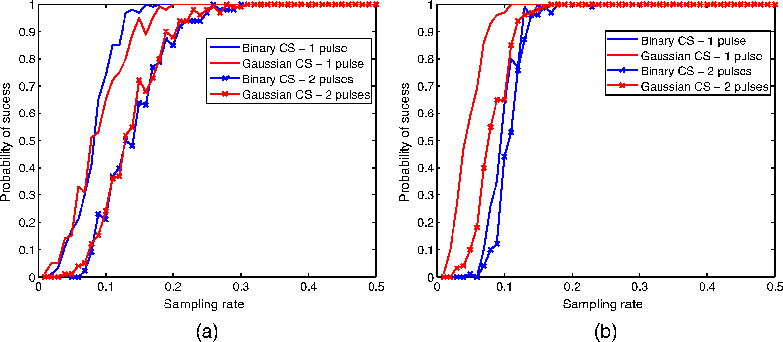

Concerning the performance of the Gaussian and the binary sensing matrix, we observe that for the greedy algorithm, there is no significant difference between the two approaches, while for lasso, the use of a Gaussian sensing matrix results in a performance gain over the use of a binary matrix. Furthermore, we validate that increasing the sparsity of the signal also has a positive impact on the performance. However, we observe that this impact is smaller for the lasso compared with OMP. Hence, in CGRS, we employ (a) a binary sensing matrix, and (b) lasso with non-negativity constraints as the recovery algorithm. In this particular scenario, we expect to be able to “perfectly” recover the ideal depth signal from sampling rates as low as $r=10\%$. The results presented in the next section confirm the theoretical prediction.

5.

Simulation Results

To validate the merits of the CGRS architecture, comparison with two state-of-the-art approaches, namely TS and gate coding, was considered. To acquire an informed understanding of the behavior of each system, the highly detailed simulator discussed in Sec. 3 was utilized. The system was set such that depth information in the range from 500 m to 2.5 Km was captured with a depth resolution of $20\mathrm{m}/\mathrm{bin}$, while the camera gating and the pulse duration were set to 100 ns. Furthermore, the backscatter coefficient was set to ${10}^{-5}$, and the attenuation factor was set to ${10}^4$. In our experiments, we considered two cases concerning the signal-to-noise ratio (SNR), namely a high SNR (30 dB) regime and a medium SNR (20 dB) regime. LIDAR data from St. Helens mountain provided by U.S. Geological Survey were used in the analysis.

In order to validate the merits of the proposed range imaging architectures, we measured the reconstruction error of each approach at various sampling rates. The sampling rate corresponds to the number of acquired frames over the total number of frames required for sampling the depth signals at the Nyquist rate. In other words, for 100 depth bins resolution, as it is the case in the experimental results, 1% sampling rate corresponds to 10 frames. The reconstruction performance is measured by averaging the Hamming error, a well-known metric that counts the number of locations where two binary vectors differ. In our scenario, each pixel is associated with a vector of length equal to the number of depth bins. This vector contains nonzero elements only when the power of the signal is above a threshold (10% of the maximum signal power), otherwise it is considered noise and is set to zero. For the single pulse case, each such vector contains a single nonzero value at the element that corresponds to the estimated distance between the camera and the object. In the perfect reconstruction case, the estimated and the true vectors have nonzero elements at exactly the same locations for all the pixels, leading to a Hamming error equal to zero, while in the other extreme, when all the elements are different, the Hamming error is one.

5.1.

Single Reflection Reconstruction

First, we consider the performance of the proposed and the two state-of-the-art GRI architectures for the reconstruction of single pulse depth signals under various conditions. Figure 5 presents the depth signal reconstruction quality as a function of the sampling rate for two SNR cases. Overall, the results suggest that CGRS is able to achieve high quality reconstruction, closely followed by GC, while TS comes last in terms of performance under the same conditions. More specifically, in these results one can see that CGRS achieves a lower error compared with GC from the low to very high sampling rates while on the other hand, GC exhibits a very stable performance. This behavior can be explained by considering the reconstruction process of each approach.

Fig. 5

Reconstruction error as a function of sampling rate for the single pulse case for signal to noise ratio (SNR) equal to (a) 30 dB and (b) 20 dB.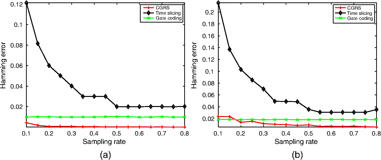

CGRS relies on a CS-based recovery approach for the estimation of the depth signals. The recovery capabilities of CS exhibit a phenomenon known as “phase transition,”³⁵ where recovery is impossible without sufficient many measurements, while as soon as the number of measurements become adequate, error-free recovery can be achieved almost instantly in the noise-free case. We can visually verify this theoretical prediction by observing that at the high SNR case, the reconstruction error is very low, even at low sampling rates, while in the noisy case, increasing the number of measurements has a positive effect on performance. On the other hand, GC requires a very small number of frames for decoding the depth signals, but reconstruction is not improved by increasing the sampling rate. With respect to the behavior of the systems under noisy conditions, we observe that CGRS and GC show a robust behavior, in contrast to the classical TS approach. Again, we can attribute this behavior to the decoding process of each approach, where CS is known to be very robust in noisy conditions. Similarly, the noise does not seem to affect GC since the maximum likelihood type decoding is also robust under noisy conditions.

Figure 6 showcases the original rendering of the depth profile, as well as visualizations of the three reconstructed range images at $r=0.2$ in the higher SNR (30 dB) case. Regarding the reconstruction achieved by TS, one can easily notice the “band” effect where points that belong to a range of distances are grouped together. This phenomenon is attributed to the coarse quantization that is required for the extraction of the scene’s depth characteristics from a very low sampling rate. On the other hand, GC and CGRS achieve superior reconstruction quality, very close to the fully sampled signal, even at this very low sampling rate.

Fig. 6

Three dimensional (3-D) depth reconstruction for the original data (a), via time slicing (TS) (b), gate coding (GC), (c) and the proposed CGRS (d), with $r=0.2\%$ at 30 dB SNR. The reconstruction error for the three methods, measured in Hamming error, is 0.06, 0.01, and 0.007 for TS, GC, and CGRS, respectively.

5.2.

Multiple Reflection Reconstruction

In addition to the estimation of a single reflected pulse discussed in the previous section, CGRS is also capable of recovering multiple reflected pulses at each imaging detector. Figure 7 presents the reconstruction quality for the multiple reflected pulses situation (two pulses received for each pulse transmitted), as a function of the sampling rate for two SNR cases. In this situation, we assume that 40% of the signal’s energy is absorbed by the intermediate surface, and the rest propagates and reflects from the objects in the scene. Our particular model assumes that a semi-transparent layer is located at 60 m distance, which absorbs 40% of the laser pulses energy, and the rest propagates and reflects from the objects in the scene.

Fig. 7

Reconstruction error as a function of sampling rate for SNR equal to (a) 30 dB and (b) 20 dB, for two pulse reconstruction.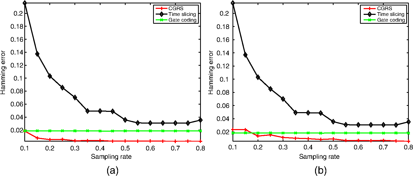

The robustness and increased recovery capabilities are easily observed in Fig. 7 for both 30 and 20 dB cases. More specially, we observe that in both cases, the typical TS approach leads to substantially worse performance than GC and CGRS. Comparing the performance with the single pulse case, we observe that TS is heavily affected by the scene’s characteristics and the image acquisition quality. Regarding CG and CGRS, we observe that with the exception of extremely low sampling rates and low SNR, CGRS outperforms GC in terms of recovery performance. Similarly to the single pulse case, CGRS is able to achieve a very low reconstruction error, even from sampling rates as low as 20%, while GC’s performance remains stable, despite increasing the number of acquired frames.

Figure 8 presents a visual illustration of the multiple reflection depth profile of the scene and the renderings of the reconstructions achieved by the three competing methods, namely TS, GC, and CGRS at $r=0.2$ sampling rate. With respect to the performance of TS, we observe that the system is able to correctly identify the two surfaces in the scene, although the particular sampling mechanism leads to a low depth resolution due to the “band” effect, which was also observed in the single pulse case. On the other hand, the architecture of GC prevents the method from correctly identifying the multiple reflected pulses, especially in situations where the two pulses are close. As a consequence of the mixing of the two signals, the GC in some cases reconstructs an artificial surface that is a composition of the two underlying sources. We observe that CGRS is able to correctly estimate the multiple reflected pulses and produce a high resolution depth description of the scene.

Fig. 8

Recovery of multireturn depth signal, shown in (a), at 30 dB SNR and $r=0.2$ by (b) TS, (c) GC, and (d) CGRS. The Hamming error is 0.103, 0.018, and 0.005 for TS, GC, and GCRS, respectively. In this case, each pixel is associated with two reflected pulses.

5.4.

Resolution Dependence

As a last important study, we analyze the resolution that each method can provide given a predefined number of frames. Figure 9 presents the reconstruction error as a function of depth resolution for a fixed set of 20 frames, for the estimation of (a) a single pulse per pixel and (b) two pulses per pixel in a high SNR (30 dB) scenario. Note that depth resolution, which is the number of individual depth bins that can be extracted for a specific distance range, is one of the most important characteristics of a GRI system, due to its relationship with the quality of the depth profile and the capabilities for further processing.

Fig. 9

Reconstruction error for varying depth resolution for a fixed frame budget (20 frames) in the (a) single and (b) two sparse signal recovery cases.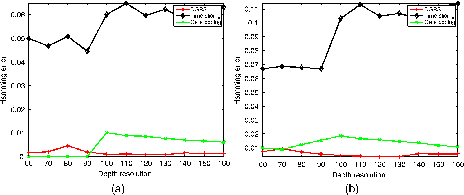

The results shown in Fig. 9 are very interesting since they highlight the behavior of each architecture. In general, for a fixed frame budget, we expect that increasing the resolution will result in lower reconstruction quality and higher estimation error. This is, indeed, the case for the TS approach where increasing the requested resolution leads to more coarse groups of depth ranges, and thus lower depth quality. On the other hand, GC is designed to achieve excellent reconstruction, provided a sufficient number of frames are available for decoding the acquired signal and under the assumption of a single reflected pulse.

In contrast with TS and GC, CGRS exhibits a very interesting property concerning the reconstruction capabilities of the method for an increasing depth resolution. Following the theoretical justification of CS, increasing the depth resolution while keeping the number of nonzero elements constant (number of reflected pulses) leads to an increase in the signal sparsity. As a consequence of the increased sparsity, the recovery mechanism is able to improve its performance and reduces the estimation error.

6.

Conclusions

In this paper, we proposed a novel application of CS for the acquisition of range images by GRI cameras. The proposed CGRS architecture is based on the ToF depth measurement principle and is able to reconstruct the depth profile of a scene with minimum reduction in quality from significantly fewer measurements, compared with traditional ToF imaging approaches. Furthermore, CGRS is capable of recovering multiple reflected pulses, which can be caused by semi-transparent elements, and thus offering a true three-dimensional profile of the scene. To achieve this goal, CGRS employs a random gating mechanism, in combination with state-of-the-art reconstruction algorithms based on the $l_1$ minimization framework for recovering multiple reflected pulses at any given location. Furthermore, unlike previous work, a highly detailed analysis of the various effects that are inflicted on the ideal depth signal, is considered and utilized by the CGRS. To validate the merits of the proposed system, highly detailed simulation scenarios were considered where numerous system parameters are taken into account. Results suggest that CGRS is a viable choice when a single reflected pulse per pixel is assumed, while it achieves superior performance when multiple reflections are considered without introducing extra acquisition costs.

This work was funded by the IAPP CS-ORION (PIAP-GA-2009-251605) grant within seventh framework program of the European Community and by the PEFYKA project within the KRIPIS action of the General Secretary of Research and Technology, Greece.