1.

Introduction

The field of self-mixing (SM) interferometry has been growing since the mid 1960s, with significant growth in the late 2000s due to better fabrication techniques of semiconductor lasers, which has opened up the possibilities to work with cheaper and higher-quality lasers in a wide range of applications. The SM effect leads to a precise and accurate metrology instrument for different purposes, such as distance measurements,¹ vibration detection,² and velocity characterization for solids,³ liquids,⁴ and plasmas.⁵

Gas targets are used for a number of accelerator based experiments, as well as for beam diagnostic purposes. In the case of supersonic gas jets, they combine low internal temperatures with high directionality, and as a result, they are very interesting as experimental targets in different fields of science.⁶ For the optimization and verification of the properties of such a monitor, it should be characterized with high accuracy, in particular with regard to its velocity and density profile. In these applications, gas jet velocities can be up to $2000\mathrm{m}/\mathrm{s}$ and can be inhomogeneously distributed across the jet. However, all currently used methods for such a characterization are either not reliable^7,8 or require a powerful laser system.⁹

At the Cockcroft Institute, a new type of ionization beam profile monitor was devised and developed utilizing a supersonic gas jet. The monitor is based on a neutral gas, shaped into a thin sheet, a fraction of which is ionized when it crosses the beam. Gas ions, created in the jet, are then extracted, allowing two-dimensional beam profile imaging.^10,11

The gas jet consists of a high density (${10}^9$ to ${10}^{12}\text{particles}/{\mathrm{cm}}^3$) of neutral molecules, which could be molecular nitrogen, argon, or helium. The gas-jet curtain is expected to have a velocity range of 100 to $2000\mathrm{m}/\mathrm{s}$, and the diameter of the jet itself is 1 to 20 mm. The characterization of the gas-jet curtain is important for further calibration of the beam monitor, so the velocimeter should measure the velocity in that range together with the density. Moreover, it is desirable to have a sensor that could be easily integrated into an existing setup with minimum additional optics components due to the complexity of the setup itself. For example, often used methodologies, such as particle image velocimetry,¹² particle tracking velocimetry,¹³ and laser speckle velocimetry,¹⁴ which have a similar working principle and are based on analyzing the net displacement of moving particles, and interferometric and absorbing techniques¹⁵ are not applicable for use in a gas-jet setup due to the complexity of installing them into an existing system.

The SM scheme can be employed in nearly every situation a traditional interferometer (such as the Michelson or the Mach-Zender interferometers) can. The main advantage of the SM scheme with respect to traditional methods is the possibility of an unambiguous measurement from a single interferometric channel. Sensors based on SM compared to other techniques are compact, have a much lower cost, and are easier to align.

The SM effect implies that the light from the laser is reflected on the target back into the laser cavity. The phenomena can be referred to as an optical feedback, induced-modulated interferometer. In the case of semiconductor lasers, the theory is different from the SM effect in gas (${\mathrm{CO}}_2$, HeNe) lasers where it was initially observed.^16,17 Specifically, the nonlinear nature of the semiconductor active medium coupled to the optical gain and refractive index to the carrier density leads to different equations and solutions resulting in unique effects.

The physics of the SM technique is such that the precise measurement of small changes in the target position is straightforward to perform. As a result, the effect was mainly applied to precise and accurate measurements of vibrations, small displacements, and the study of slow movements. The measured velocities reported in the literature using the SM technique rarely exceed $5\mathrm{m}/\mathrm{s}$ (Refs. 3, 18, and 19) with several works mentioning the movement of solid object by $25\mathrm{m}/\mathrm{s}$ (Ref. 20) and $55\mathrm{m}/\mathrm{s}$.¹⁵

SM interferometry has been applied to flow-velocity measurements often aimed at biological applications, such as blood flow characterization,²¹ Brownian motion, and biological species dynamic studies, widely presented in the review by Otsuka.⁴ However, all of the objects considered in these cases of velocity characterization move relatively slowly. Such a high interest in this area has resulted in a number of works with measurements of relatively small velocity from $0.1\mathrm{mm}/\mathrm{s}$ to $10\mathrm{cm}/\mathrm{s}$ (Refs. 22 and 23) with high accuracy.

Most work has been focused on the precision of such measurements providing a high spatial resolution. Using solid or liquid targets leads to a higher backscattered intensity as compared to gas targets; on the other hand, typical velocities of interest expected for a planar gas jet are at least in the range $0.5<M<4$, where $M$ stands for the Mach Number; when translated to $\mathrm{m}/\mathrm{s}$, this gives a range of roughly 100 to $2000\mathrm{m}/\mathrm{s}$,²⁴ which has previously not been explored.

The motivation of the present study is to clarify the possibility of measuring high-speed velocities up to $50\mathrm{m}/\mathrm{s}$ in the geometry of the gas-jet setup, Secs. 3.1 and 3.2, with solid objects, and the possibility of measuring fluid velocity up to $100\mathrm{cm}/\mathrm{s}$, see Sec. 3.3.

2.

Methodology

The first analysis of the SM phenomena in the case of a laser diode (LD) was performed by Lang–Kobayashi.²⁵ A useful review of the theory and practical approach to the SM effect in semiconductor lasers is given in the book,¹⁸ demonstrating theoretical investigations into SM and developments of various applications.

The working principal of the system is that the light from the laser scatters off the target and the scattered light returns back into the laser cavity. The laser plays the role of a coherent heterodyne receiver and amplifier of the signal, and at the same time, the quadratic detection of the registered signal is inside the laser. The behavior of the system can be described in different ways. The target can be seen as an additional mirror for the laser system, and then the system is a known three-mirror laser, where the laser has an external cavity with a length of the distance between the laser and the target, often called the theory of the equivalent-lens cavities.²⁶ From this point of view, the SM system can be described by a set of field and rate equations obtained by adding an additional external feedback term to the standard equations.^25,27 Another approach is to consider the system as a two-mirror laser with a modified complex reflection coefficient or effective reflection coefficient, and use solutions derived for LD systems.³ As a result, the solution is based on replacing the parameters without feedback with parameters that depend on an additional mirror (target).²⁸

Within both ways of describing the system, the modulation of light as a result of the interaction with the target can be mathematically described by

$P_0$ and $P$ are the optical powers without and with feedback, $m$ is a modulation parameter, $F$ is the self-mixing interferometric waveform, ${\tau }_D$ is the time of flight of the wave, and $\upsilon$ is the frequency of the laser light undergoing feedback. The modulation index $m$ and the shape of $F$ are the function of the feedback parameter $C\propto r_{3}D$, so that $C$ depends both on the level of feedback (the portion of light that returns back to the laser cavity), which is defined by the reflectivity coefficient $r_3$ together with coupling optics, and on the target distance $D$.^3,27,28 There are four different types of signals in SM depending on the amount of backscattered light coupled into the cavity, see Fig. 1. In the case of a low amount of back-injected light (weak feedback, $C\ll 1$), the signal is a sinusoidal and the function $F$ is cosine. Gradually increasing the level of feedback, the shape of the signal can be deformed from a sinusoidal ($C\ll 1$) to a nonsymmetrical sinusoidal-like shape ($0.1<C<1$) and then into an asymmetrical sawtooth-like form ($C>1$). The orientation of the function $F$ depends on the sign of the phase, so the direction of the target movements can be discriminated.^29–31 Figure 1 demonstrates the example of the SM signals together with the principal of direction determination. In both Figs. 1(a) and 1(b), the two top plots represent the case with the targets approaching the laser, and the two bottom plots represent that of the target moving away from the laser. The signals in the middle with $C<1$ are close to a sinusoidal shape.

Fig. 1

Experimentally obtained self-mixing signals for two different types of surfaces: (a) mirror and (b) white paper when the translational stage was moving with a velocity of $5.00\mathrm{cm}/\mathrm{s}$ toward (top plots) and away (bottom plots) from the laser. The plots are shifted along the $y$ axis, so the comparison of the shapes of self-mixing (SM) signals is possible as a function of the level of the feedback re-entering the cavity. The coupling efficiency is related to the coefficient $C$. The plots in the middle with $C<1$ correspond to weak feedback, and the shape of the signal is close to sinusoidal. As the amount of light coupling back into the cavity increases, the shape of the signal distorts and becomes a nonsymmetrical sinusoidal signal with $C\approx 1$. In the case of strong feedback ($C>1$), which is shown in the top and bottom plots in both (a) and (b), the signal is sawtooth-like. In the case of an asymmetrical shape of the signal, the direction of leaning denotes the direction in which the target was moving. The top plots lean to the left corresponding to when the target is moving toward the laser diode (LD). The bottom plots, where the signal is leaning to the right, are when the target was moving away from the laser. In case of the white paper (b), the signal amplitude is slightly reduced and distorted in shape as a result of speckle effects, though the shape and trends are the same with the mirror (a) as a target.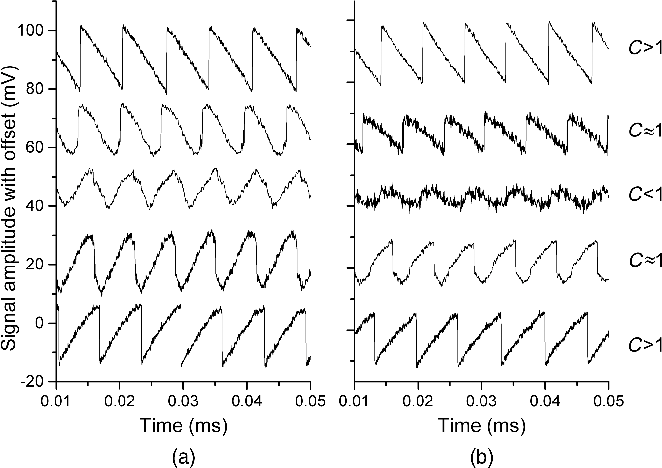

The velocity can be calculated from the spectrum of the power of the signal. As previously mentioned, the signal is the result of mixing the initial lasing field and the Doppler shifted backscattered light. The power spectrum of the laser changes due to interaction between the lasing field and the small backscattered field, which re-enters the laser cavity with results described by Eq. (1). The Doppler shift of the periodic optical power fluctuation ($f$) is equal to

In the case of mirrors or other surfaces with low roughness, the specular (mirror-like) reflection prevails over the diffuse reflection. As a result, the level of the feedback in the case of alignment is very high and leads to cases with $C>1$. Using additional filters, it is possible to have a system with weak feedback.

Using a rough surface as a target for SM, it is possible to apply the SM technique without additional alignment, so it can be performed at any angle. Light scatters off a rough surface in all directions; this is in contrast to smooth surfaces where light reflects mainly in one direction. However, due to random interference of light scattered off the rough surface, speckles³³ are observed affecting the shape of the SM signal received, causing an error in the measurement.³⁴ An ideal case of an SM signal is a harmonious function with constant amplitude with a narrow spectral line in the spectrum. In the presence of speckles, the amplitude and the phase of the SM signal is modulated, which leads to spectral broadening and additional noises in the signal.³⁵

The speckle phenomena in SM can be used not only for a displacement measurement,³⁶ but also for the surface classification³⁷ as well as for the length of the moving objects.³⁸

When the light travels through a liquid or gas, the interaction between the light and particles randomly changes the phase and amplitude of the scattered light.³³ The power spectrum [Eq. (1)] provides information about the scattered particles, such as velocity, along the laser light axis and other properties, such as the concentration in the volume and their size.³⁹

3.

Experimental Results

The SM technique can be applied using any type of laser, and both the target and property of the laser itself should be correctly taken into account. In the case presented here, the experiments were performed using an LD with 650 nm wavelength (L650P007) with a power of $<5\mathrm{mW}$, driven by a constant current. The light was focused onto the target by a lens with numerical aperture 0.26. The signal was received from the built-in photodiode, which is usually used for monitoring the LD. The current was amplified and modified into a voltage signal by a transimpedance amplifier produced by Femto (DHPCA 100). The velocities of the targets were calculated by performing a fast Fourier transformation (FFT) of the voltage signal applying Hamming and Blackman-Harris windows. The spectrum was processed with a smoothing filter, and the peak of the spectra was found by fitting a Gaussian distribution in the frequency domain.

The following subsections are divided into three parts, with each subsection devoted to a different investigated target: a mirror with a high reflective index mounted on a translational stage, a diffusive surface (white paper) first mounted on a translational stage and then on a rotational disc, see Figs. 2(a) and 2(b), and, finally, milk diluted in water and also a titanium dioxide (emulsion paint) water solution measured by means of laminar flow out of a hose, see Fig. 2(c). The right part of Fig. 2 demonstrates the projection of the targets’ velocity in different experimental setups. Only that component of the velocity that lies on the laser axis interacts with the laser light.

Fig. 2

Illustration of the layout of the experiments on the left side, and the schematic illustration of the projection of the velocity on the laser axis for each case on the right side. The light from the LD is focused by means of multiple lenses onto a target. Light then scatters off the target and is coupled back into the laser cavity, leading to an SM effect. A signal is produced by an inbuilt photodiode (PD), and amplified and converted into a voltage signal by an amplifier. Three experimental setups were established for testing the SM velocimetry technique: (a) the translation stage; (b) rotating disc; and (c) fluid stream. The translation stage (a) moves the target (mirror or white paper) toward and away from the laser; as a result, the scattered light has a Doppler shift proportional to the velocity vector in the direction of movement. In the case of rotating disc (b) covered with white paper, the direction of the rotation defines the direction of the velocity vector relating to the laser axis. The velocity vector has its projection on the laser axis depending on the incident angle. The fluid (c) disgorges from the nozzle, so the flow is laminar. The laser light shines at an angle to the velocity [${\alpha }_{\mathrm{f}}$ in (c)], so the measured velocity is the velocity projected onto the laser axis.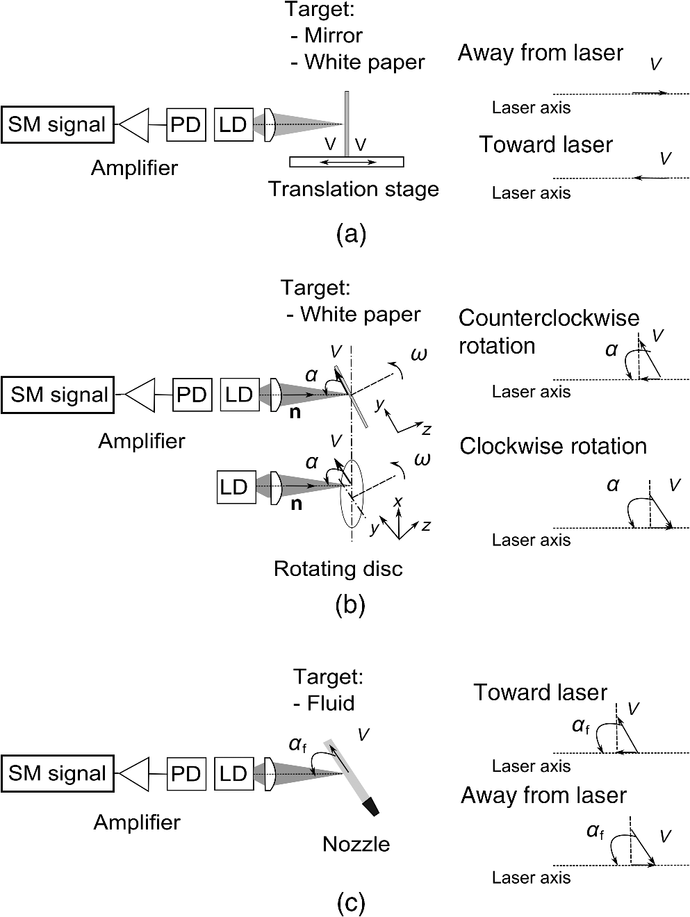

3.1.

Moving Target with Different Reflectivity

First, the experiments with a mirror and with white paper were performed using the same setup, where the target moves back and forth on the laser light axis, see Fig. 2(a). The target was moved by a stage driven by a direct current motor controller, which gives precise velocities in the range of 0.01 to $10.00\mathrm{cm}/\mathrm{s}$. In the case of the mirror, all four feedback regimes, mentioned earlier, were observed and studied depending on how focused/defocused the light was on the target. Figure 1(a) demonstrates different types of SM signals and the distortion of the shapes of the signal depending on the amount of light coupling back into cavity. In the case of moderate ($C>1$) and weak feedback ($0.1<C<1$), both the velocity and its direction were measured with high accuracy. The reflectivity coefficient directly influences the feedback parameter and, thus, the performance of the SM technique. The refractive index depends on the real refractive index and light absorption coefficient. Reflectivity is a function of the refractive index and incident angle. The reflectivity of the aluminum mirror at the normal angle for 650 nm is $\sim 92\%$. In order to reduce the amount of light coupling into the laser cavity, density filters were used. Experiments with a mirror, which moves across the transverse axis of the laser beam, were performed to understand the SM technique as a whole, such as the best geometry of the setup, reduction of the noise level, the focusing/defocusing properties of the LD, and the investigation of the system itself. In the case of a well-adjusted setup, the mirror target was moved up to 90 cm from the laser without changing the shape of the signal [Fig. 1(a), regimes with $C>1$]. The experiments demonstrated that accurate velocity measurements with a precision of $>1\%$ can be obtained at a distance up to 90 cm from the target.

With a rough surface target, such as paper, weak or moderate feedback is expected due to a lower reflectivity equal to $\sim 60\%$ when normal to the surface for laser light of 650 nm. Typical examples of the signals received with white paper are shown in Fig. 1(b). The signals are similar in shape and the precision of the methods are the same in both cases. However, the amplitude of the signal is less when compared with the same type of signals in the mirror experiments. The size of the laser spot on the white paper required readjustments while the distance between the LD and target was changing. Using the mirror as a target allowed measurements up to 90 cm from the target without changing anything in the setup; however, when using the white paper as a target, readjustments were required periodically up to 50 cm where no signal was detected.

Accurate measurements with a $>1.5\%$ precision of the velocity were obtained in the range of 0.01 to $10.00\mathrm{cm}/\mathrm{s}$ at a distance up to 50 cm between the LD and the white paper target. The results of the measurements are presented in Fig. 3, which shows both the accuracy and precision of the measurements. The thin straight solid line is a reference velocity, and the measured velocity is shown with associated error bars, which give the range within which the measured velocities were obtained over multiple readings. The dashed lines represent the measured velocity in the SM signal at different distances up to 90 cm from the laser with a mirror as a target, and the solid line shows a measured velocity using the white paper as a target.

Fig. 3

Example of measurements from the experiments using a movable stage, which allows for a precise velocity measurement (straight solid line) in the range of 0.01 to $10.00\mathrm{cm}/\mathrm{s}$ with a mirror (dot lines) and white paper (thick solid lines) with an error bar obtained at different distances between the laser and the target. The velocity measurements were carried out up to 90 cm for the mirror and 50 cm for the white paper and showed a better than 1% accuracy and 1.5%, respectively. The error bars indicate the range of the measured velocity obtained in different independent sets of experiments.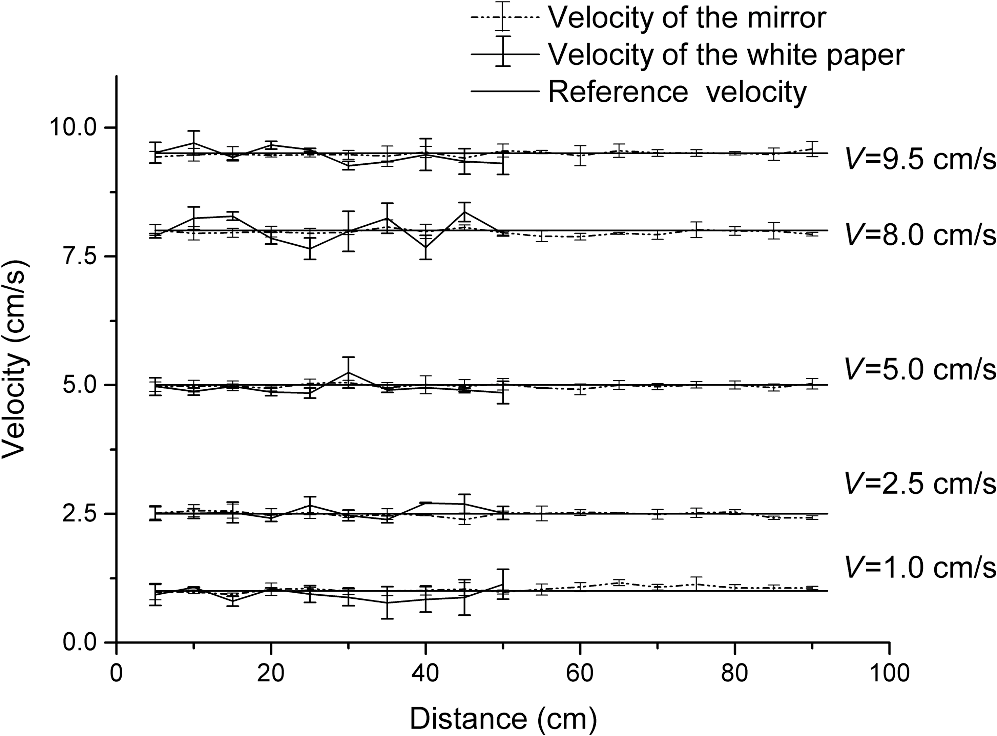

3.2.

Rotating Target with Low Reflectivity (60% at 650 nm)

A rotating disc was then covered with white paper, allowing the limitations of the setup to be investigated at high velocities. The distance between the target and the laser was fixed to 10 cm in the geometry shown in Fig. 2(b). This distance was selected as this is the expected distance when the velocimeter will be installed into the gas-jet setup. The rotational speed $\omega$ of the disc can vary from $2\pi$ to $300\pi \mathrm{rad}/\mathrm{s}$ which translates into tangential velocities $V$ from $1\mathrm{cm}/\mathrm{s}$ to $100\mathrm{m}/\mathrm{s}$.

The white paper has micrometer (40 to $50\mu \mathrm{m}$) surface roughness. The power spectrum of the light scattered off rough surfaces is anticipated to be Gaussian with a frequency corresponding to the Doppler shift of the SM system. The reflectivity properties of the white paper are such that 60% of the light, with a wavelength of 650 nm, is expected to scatter. The amount of light scattered in different directions depends on the incident light angle with a maximum at 90 deg.⁴⁰

Different points on the rotating disc move at different tangential velocities $V$. The motion can be characterized by the rotational speed, which is given by revolutions per second, $\nu$. The tangential velocity $\overrightarrow{V}$ is perpendicular to the diameter of the disc at each point and at a tangent to the circle. The tangential velocity of the point at the radius $R$ of the disc is $V=\omega R$, where $\omega$ is $2\pi \nu$. The laser is turned to an angle $\alpha$ in order to have a vector of velocity, which would not be equal to zero in relation to the laser beam axis. The right part of Fig. 2(b) illustrates this concept, showing the projection of the velocity on the disc depending on whether the rotation is clockwise or anticlockwise when the laser spot is above the point of rotation, i.e., the center of the disc.

The Doppler shift for the SM system can be described by Eq. (2), where the velocity vector of $\overrightarrow{V}$ and the unit vector $\overrightarrow{n}$ can be described differently depending on the position of the laser spot.

The co-ordinate system is defined to be $x\text{-}y$ on the surface of the disc with the origin at the center, and $z$ is parallel to the normal vector of the disc surface. In Fig. 4(a), for vectors $\overrightarrow{V}=V(\mathrm{0,1},0)$ and $\overrightarrow{n}=(0,\cos \alpha ,\sin \alpha )$, the Doppler shift is equal to $f=2\omega R\cos \alpha /\lambda$. In the case when the laser is shining on any point on the disc surface [see Fig. 4(b)], the vector $\overrightarrow{V}$ is given by $\overrightarrow{V}=V(\sin \beta ,\cos \beta ,0)$. Thus, the Doppler shift in the most general case is equal to

Eq. (3)

$$f=\frac{2\omega R\cos \alpha \cos \beta }{\lambda }.$$

Fig. 4

The laser light from the LD is focused by means of multiple lenses onto a point on a rotating disc located a distance $R$ from the point of rotation. The origin of $x\text{-}y\text{-}z$ coordinate system is defined to be at the point of rotation of the disc. $\overrightarrow{n}$ is a unit vector in the direction of propagation of light, and $\omega$ is the rotational speed of the disc. (a) In the case of the laser shining onto any point on the $x$ axis, the Doppler shift depends only on the angle $\alpha$ between laser light direction and the disc surface ($y$ axis). (b) At any other point, the Doppler shift depends on the angle $\beta$ between the velocity vector and $y$ axis.

The variation of the velocity can be achieved by changing the revolution per second ($\nu$), the position of the laser spot on the disc (which will change the radius $R$), and the angle $\alpha$.

In order to validate the results of the measured SM system, a photointerrupter circuit based on the OPT101 photodiode amplifier from Texas Instruments and a microcontroller board (ATMega 328) were used for measuring the rotational speed of the motor.

From every measured signal, a corresponding frequency spectrum can be found, and by using Eq. (1), the velocity can be calculated with a reference velocity based on Eq. (2). The uncertainty of the radius $\mathrm{\Delta }R$ is defined as the size of the laser spot on the paper; all other errors are limited by the instrumentation. The relative error on the reference velocity can be calculated by differentiating Eq. (2) with the angle variation between the laser and the disc giving the most significant uncertainty. The experimental uncertainty of the velocity, based on the uncertainties in the experimentally measured quantities, was calculated according to $\delta V\text{laser}=\sqrt{{(\delta R)}^2+{(\delta \nu )}^2+{(\delta \alpha )}^2}$, where $\delta R=\mathrm{\Delta }R/R$, $\delta \nu =\mathrm{\Delta }\nu /\nu$, and $\delta \alpha =\tan (\alpha )\mathrm{\Delta }\alpha$. The calculated dependency on the velocity uncertainty of the setup from the angle is shown in Fig. 5 with a solid black line with a 5% level of the accuracy by the dashed line. For calculations, it was assumed that the angle could be measured with a 0.5 deg precision. The rotational velocity $\omega$ was defined with an accuracy of 1%. The size of the laser spot on the paper depends on the angle $\alpha$ as well being proportional to the cosine of this angle, leading to an increasing relative error of the measurements at small, $<10\mathrm{deg}$, angles due to a broadening of the frequency spectrum. Speckle modulation increases dramatically at angles $>80\mathrm{deg}$, which also results in frequency spectrum broadening.^19,35 Considering the trend of the calculated experimental uncertainties, presented in Fig. 5 by a black solid line, the optimal range of angles from an accuracy point of view is between 13 and 77 deg, which gives an error of $<5\%$, and between 25 and 63 deg, which gives an error $<3\%$.

Fig. 5

The theoretical and experimental relative error dependence on the angle between the disc covered with white paper and the laser. The theoretical error was calculated as the uncertainties in the experimentally measured quantities (see Sec. 3.2) and shown by the solid line. The experimental accuracy is shown by the dashed line with round dots, which represents the mean accuracy calculated from multiple readings over a range of velocities. The error bars on the experimental plot represent the range of the measured velocities obtained after set of independent experiments and demonstrate the precision of the results. The experimental results follow the same trend as the theoretical one. In the range of 15 to 85 relative errors were better than 5%, and the most precise measurements were received in the range of 30 to 75.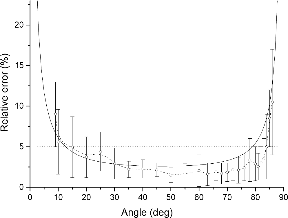

During the experiment, the following parameters were varied: the position of the laser spot on the disc, the angle $\alpha$, and the rotational speed of the disc. Figure 5 represents the results of the accuracy, which was achieved during the experiments for different angles, shown by a dashed line. The accuracy of the measurements was defined as the relative error in relation to the reference velocity. For each angle taken in the plot, multiple measurements were taken over a velocity range of 0.5 to $30\mathrm{m}/\mathrm{s}$ with at least 10 measurements for each velocity. The points in Fig. 4 represent the average of the uncertainty over the velocity range for each angle. Along with the accuracy of the measurements, the error bars are presented for each point, which represents the precision of the independent measurement within the total accuracy of the results.

The experimental accuracy follows the same trend as the theoretical one in Fig. 5 with sharp improvements of the accuracy starting from an angle of 15 deg with a plateau of 3 to 4% of the accuracy in the range of 25 to 80 deg and with a rise of inaccuracy above 85 deg. The error bar for each point in the plot shows that the precision of the measurements improves within the range of 25 to 75 deg. The calculated velocity is based on the frequency extracted from the signal spectrum. In the case of a movable mirror, the whole surface moves with the same velocity. As a result, the peak of frequency is quite narrow, even if the spot of the laser light is nonpoint-like. Each point on the disc, however, has a different velocity. The laser spot has a finite size, i.e., it is nonpoint-like; this means that for each point on the disc, a different tangential velocity is measured, which results in a distribution of velocities with different weights in the signal measured. This can be seen by a broadening of the signal spectrum.

Figure 6 demonstrates typical waveforms and their FFTs in the case of an accuracy $<5\%$ [Fig. 6(a), 1.4% accuracy] and $>5\%$ [Fig. 6(b), 6.7%]. The signals were chosen such that the peaks of the FFTs are relatively close to each other for comparison. The Doppler shifts are 3.41 MHz for Fig. 6(a) and 3.23 MHz for Fig. 6(b), which correspond to tangential velocities $V$ of 17.6 and $10.6\mathrm{m}/\mathrm{s}$, respectively, while the angle between the laser axis and the surface of the disc [see Fig. 2(b)] was 51 and 9 deg, respectively. The disc, when covered with white paper, leads to an intensity modulation due to speckle effects, which can be seen in the signal plots in Fig. 6. The signals in Fig. 6 have a shape typical for weak feedback. The setup allows calculation and verification of the SM method with velocities of up to $50\mathrm{m}/\mathrm{s}$. The only limitation of the experiment found so far is from the electrical circuit parameters (bandwidth of the amplifier). As a result, the high velocities could be measured only with a small angle and, as a consequence, with low accuracy. The experimental results on the velocity measurements with white paper as a target are shown in Fig. 7. Using a disc as a target allows the SM velocimeter to be validated. The accuracy is dominated by the angle between the target and the laser, see Fig. 5. The accuracy of the reference velocity was obtained based on the uncertainties of variables used for calculations. The measured velocity shown in Fig. 7 is an average of repeated measurements with a combined error. Starting from $20\mathrm{m}/\mathrm{s}$, only large values of $\alpha$ were used, close to the normal of the disc surface, due to the low bandwidth of the transimpedance amplifier in the readout electronics. The precision of the results are, on average, better than 6%.

Fig. 6

Examples of typical SM signals and their fast Fourier transformations received from the setup with a rotating disc for the case of a relative error (a) $<5\%$ and equal to 1.4%, and (b) $>5\%$ and equal to 6.7%. The reference and measured velocities were (a) $17.6\mathrm{m}/\mathrm{s}$ and (b) $10.6\mathrm{m}/\mathrm{s}$. The angles between the velocity vector and laser axis were (a) 51 deg and (b) 9 deg, leading to Doppler frequencies of 3.4 and 3.23 MHz, respectively. The waveforms demonstrate the intensity modulation effect due to nonpoint-like laser spot and speckle effects leading to a broadening of the frequency spectrum. In (b), the spectrum is expected to be broader due to the changing of the size of the laser spot on the disc.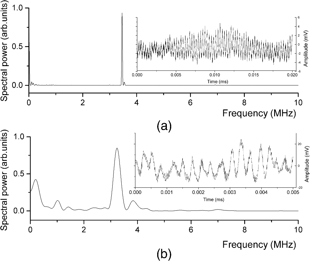

Fig. 7

Experimental results from measurements of a rotating disc covered with white paper. The difference in the resulting and estimated velocity is within the limits of uncertainty. The limitation of the velocity was due to the bandwidth of the amplifier used for the SM velocimeter. The increasing uncertainty at high speeds, equal to and higher than $20\mathrm{m}/\mathrm{s}$, is caused by the angle, $\sim 90\mathrm{deg}$, used for the measurement.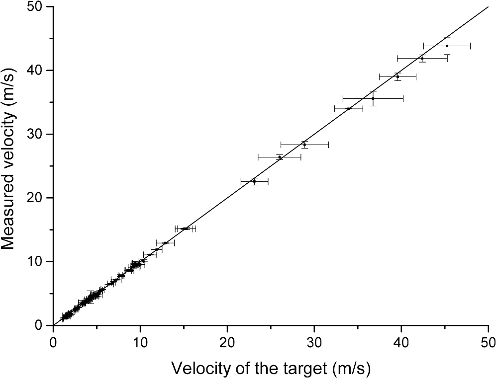

3.3.

Fluid as a Target

The next step in the experiment was to check the possibility of measuring the velocity in the case of smaller scale targets in the case of low-level feedback.

To measure the velocity of liquids, an experimental setup was established which allows measurements to be compared with analytical and numerical solutions for verification and benchmarking of the SM velocimeter.

Laminar flow was achieved by discharging liquid from a nozzle of a tube pointed horizontally into the atmosphere. The liquid flow outlet velocity from the nozzle depends on the pump power. The laser light was focused close to the nozzle, 0.4 cm from the outlet; and the direction of the velocity, ${\alpha }_{\mathrm{f}}$ in Fig. 2(c), was at an angle of 28 deg with respect to the laser light axis as seen in Fig. 2(c). The right part of the schematic configuration represents the position of the velocity vector with respect to the laser axis.

A mixture of water with milk was used for fluid velocity measurements at first. Milk was chosen as it consists of an emulsion of fat in water, where 87% of the milk itself is water, and only 4% is fat globules. The refractive index for the milk at 650 nm wavelength is 1.45 and the light absorption coefficient is $<{10}^{-5}$,⁴¹ which resulted in reflectivity of $\sim 3.5\%$.

In the first set of experiments, the velocity of the diluted milk was measured in the range between 1 and $20\mathrm{cm}/\mathrm{s}$. The distance between the LD and the target was fixed to 4 cm. The measurements were performed for 5% concentration of milk. The fat globules’ shape is close to spherical, with the average size of the molecules being 3 to $6\mu \mathrm{m}$.⁴¹

In the second set of experiments, the velocity of water seeded with titanium dioxide was measured with the same wavelength of 650 nm. A refractive index of 1.49 was calculated for the mixture based on a measurement of the critical angle from a measurement of the angle of total internal reflection. The setup was used for studying smaller-scale seeds, 0.5 to $1\mu \mathrm{m}$, allowing lower densities of the concentration, $<1\%$ of the volume, to be probed.

Since both the milk and titanium dioxide solutions appeared white, the visible light is scattered equally. Light scatters off moving particles in the fluid (the initial particles or seeds) in all directions with some angular distribution of scattering efficiencies corresponding to the properties of the scattered particles.⁴²

The SM technique allows measurements of the velocities of the solution of up to $1\mathrm{m}/\mathrm{s}$. An example of the SM signal obtained during the experiment can be seen in Fig. 8. The signal can be characterized as a signal with weak feedback. Depending on the optics used and the concentration of the seeds, the direction of the moving target was able to be defined only when the type of the SM signal corresponded to the weak feedback with $C>0.1$.

Fig. 8

Experimental setup for flow velocity measurements. The liquid flow discharges from the nozzle into the atmosphere using a controlled pump system, which allows a reference velocity to be defined. The laser light was focused on the center of the liquid flow at a distance of 0.4 cm from the nozzle outlet at 28 deg.

The velocities of fluids up to $1\mathrm{m}/\mathrm{s}$ were successfully measured with high accuracy, as shown in Fig. 9(b). The velocity was found from the averaged spectrum of 20 power spectra for each velocity on the plot. The dashed line is the reference velocity of the fluids. The differences in the resulting and estimated velocity of the fluid were within the limits of uncertainty of measurement and calculations.

Fig. 9

Experimental results from measuring the velocity of fluids. (a) Example of the signal received from the setup with a titanium oxide water solution as the target. The reference and measured velocity was $0.55\mathrm{m}/\mathrm{s}$. (b) The results of the measurements of the velocity up to $1\mathrm{m}/\mathrm{s}$ were measured with an accuracy better than 4%. Velocities in the range of 1 to $20\mathrm{cm}/\mathrm{s}$ were carried out for milk diluted in water to a 5% concentration, shown by round dots. Higher velocities, up to $1\mathrm{m}/\mathrm{s}$, shown in the graph are obtained from measurements of the titanium oxide water solution with a $<1\%$ concentration in volume and were also measured with accuracy 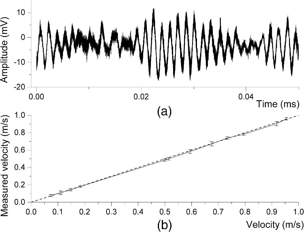$>4\%$.

4.

Conclusion and Outlook

A diode laser velocimeter based on the laser SM method has been developed as an easy-to-build and compact solution when compared to alternative measurement techniques. First tests with solid targets and fluids were carried out and the technique seems a promising way for a complete characterization of moving objects. The laser velocimeter could provide in-detail information about velocity and density of liquids and, eventually, a gas jet with micrometer resolution. Such a sensor would allow for unambiguous measurements from a single interferometric channel and could be installed even in radiation-exposed environments.

The laser velocimeter is a self-aligning device based on the SM method, where the laser is both a transmitter and receiver of the signal. It should be noted that laser SM is usually used for measurements of low velocities and vibrations. The theoretical analysis presented here shows the possibility to extend these measurement capabilities to higher velocities by altering the design.

Table 1 presents the results of the velocity measurements for different targets. In the experiments, the bandwidth of the transimpedance amplifier was 15 MHz, which was the main limitation in measuring higher velocities. Measurements of high, up to $50\mathrm{m}/\mathrm{s}$, velocities with white paper on a disc were achieved with an uncertainty better than 5%. The fluid velocity measurement showed the possibility to measure a signal with a low-level feedback with promising results of measuring high velocities, up to $1\mathrm{m}/\mathrm{s}$, which were not covered in previous studies.

Table 1

Results of the experiment with different targets with different reflectivity.

An initial calibration and verification of the accuracy of the method was performed on a setup that gave access to velocities of up to $50\mathrm{m}/\mathrm{s}$. In order to verify the possibility of using the velocimeter as a flow sensor, measurements of local velocities were performed on fluids with externally imposed flow profiles and different densities. The first experiments allowed velocity measurements of fluids up to $1\mathrm{m}/\mathrm{s}$.

First experimental results show that the velocity of a white paper target and fluids can be measured with an accuracy of $>5\%$ and micrometer spatial resolution over a velocity range from $0.5\mathrm{mm}/\mathrm{s}$ to $50\mathrm{m}/\mathrm{s}$. The sensor’s capability to measure even higher target velocities will be subject to further studies.

For the next step, it is planned to apply the above method to characterize liquids with different densities and velocity distributions, as well as ultrasonic gases. The extension of the methodology to these particular cases will have to overcome two major challenges. The first is that the intensity of the backscattered light may not be large enough, and second, the sensor may not be able to cope with velocities on the order of the speed of sound. Taking into account optical properties and density of the gas jet together with collimation optics for the LD, calculations show that, potentially, seeding techniques will need to be applied to increase the reflectivity of the supersonic jet, and this will be part of future investigations.

Successful use of SM strongly depends on the quantity of feedback coupled back into the laser cavity. It is stated¹⁵ that for the weak feedback regime to be attained, a level of feedback of $-90\mathrm{dB}$ is usually required. The required level of feedback also depends on the particular type of laser used and on the particular optics. The quality of the detectable signal also depends on the electrostatic insulation of the system and the pickup noise of the electronics. It is, therefore, necessary to set up an experiment that allows the attenuation in the external cavity leading to the different regimes to be measured, using the particular elements and external conditions of the specific laboratory. One particular area of interest in this study is to find the minimum level of concentration (the number of particles) required to be detected together with the maximum speed that can be measured. This will provide insight into the applicability of the method for targets with lower density.