Optical surface evaluation by correlating bi-Ronchigram images

Alberto Cordero Dávila; Jorge González García

doi:10.1117/1.OE.54.3.034108

16 March 2015 Optical surface evaluation by correlating bi-Ronchigram images

Alberto Cordero Dávila, Jorge González García

Author Affiliations +

Optical Engineering, Vol. 54, Issue 3, 034108 (March 2015). https://doi.org/10.1117/1.OE.54.3.034108

Abstract

By correlating bi-Ronchigram images, surface errors without any supposed symmetry are evaluated. No approximation and interference orders are needed. First, only one experimental bi-Ronchigram (Ronchigram with a square grid) image was recorded. Second, given a surface parameter set (curvature radius, conic constant, and/or symmetric and asymmetric deformation coefficients), a bi-Ronchigram image is simulated and correlated with the bi-Ronchigram experimental image. Third, genetic algorithms are used to find the parameters for which the correlation coefficient reaches its maximum value. Finally, the parameters of the experimental surface are estimated. Evaluations of curvature radius, conic constant, and error functions for reflecting surfaces will be shown.

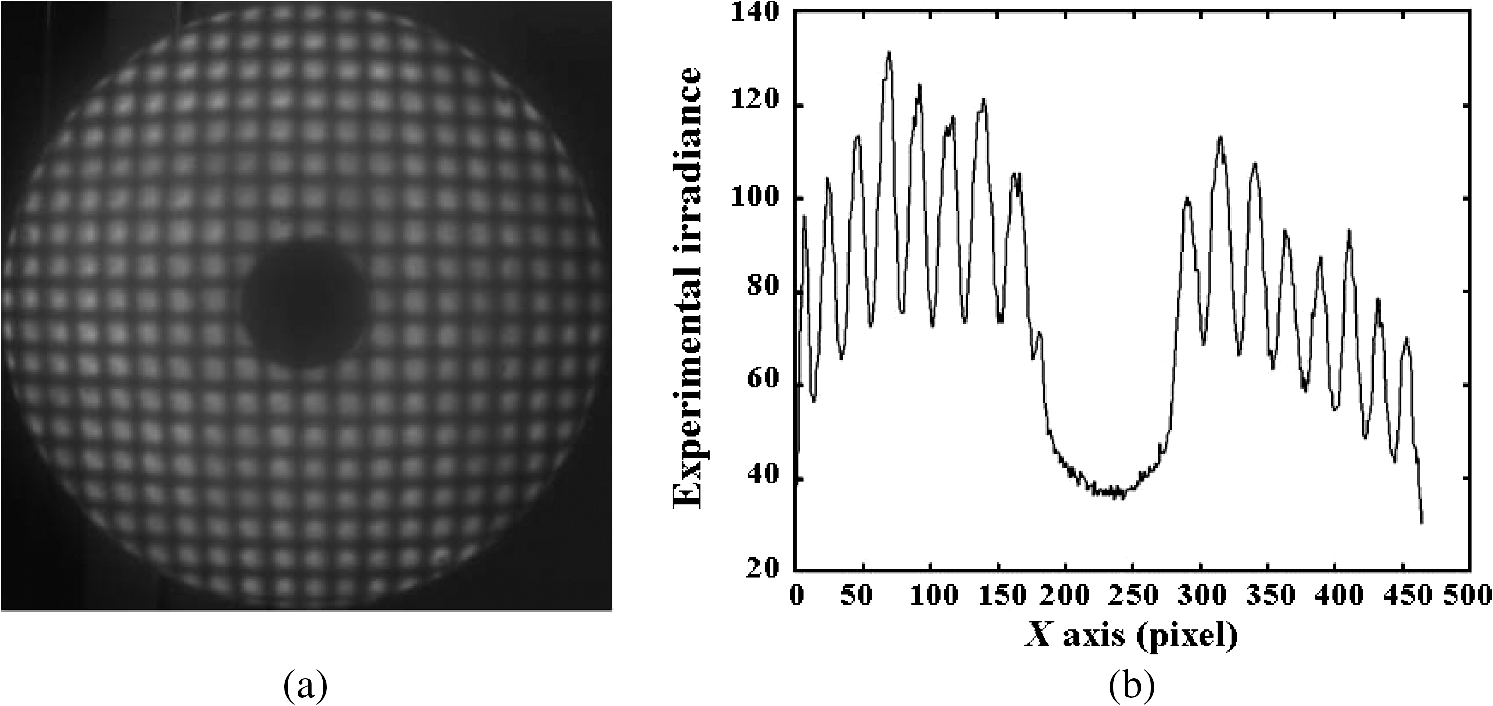
1. Introduction

In optical shops, experimental and simulated Ronchigrams¹^,² are visually compared in order to qualitatively evaluate reflecting surfaces. On the other hand, to quantitatively evaluate the aberrations of any asymmetric surface (or wavefront), two crossed Ronchigrams have to be recorded.³^,⁴ From each one, a component of the transversal aberration function is calculated.⁵^–⁷ After an analytical integration is applied³^,⁴ and the optical path differences (OPD) function is calculated, it is possible to record only one pattern (bi-Ronchigram) if a square grid is used instead of the classical Ronchi ruling.⁸ In this latter case, a numerical⁸ or analytical integration⁹ can be applied to estimate the OPD function. To evaluate phase function from a pattern of fringes,¹⁰ the correlation coefficient between the experimental and simulated interferogram is maximized by using genetic algorithms. Recently, a similar procedure has been used to evaluate Ronchigrams.¹¹

What follows in this paper is the description of a procedure to estimate parameters and error function of any kind of mirror. By using the experimental setup shown in Fig. 1, we recorded the experimental bi-Ronchigram image, which was correlated with several simulated images of bi-Ronchigrams. Before any bi-Ronchigram was recorded, the ruling was aligned in order to guarantee the parallelism between (1) ruling lines and CCD array, (2) the normal of the CCD and ruling plane normal, and (3) the normal of the ruling plane and optical axis of the mirror. For each theoretical surface used for simulation, the error function was a different one until a correlation coefficient was maximized. As a result, the parameters of the experimental surface were estimated.

Fig. 1

(a) Experimental setup of Ronchi test and (b) CCD camera, Ronchi tester ( $λ = 660 nm$ ) and square grid.

In Sec. 2, the problem is stated. In Sec. 3, the algorithm to simulate bi-Ronchigram images is described. Algorithms used to normalize experimental bi-Ronchigram images and to correlate simulated and experimental bi-Ronchigrams are described in Sec. 4. Experimental results are reported in Sec. 5. Finally, our conclusions are reported in Sec. 6.

2. Statement of the Problem

Any surface can be described by means of a vector of parameters, $a$ (curvature radius, conic constant, symmetric and asymmetric deformation constants, etc.). The experimental surface is defined by an unknown experimental vector of parameters, $a_{ex}$ , and the surface used to simulate a bi-Ronchigram image is defined by its parameters vector, $a_{s i}$ . By correlating the experimental and simulated bi-Ronchigram images, a correlation coefficient, $C (a_{ex}, a_{s i})$ , is obtained. We used genetic algorithms to find the $a_{s i}^{*}$ value for which the correlation coefficient, $C (a_{ex}, a_{s i}^{*})$ , is maximized. We assume that the best estimator of $a_{ex}$ is $a_{s i}^{*}$ and then the experimental surface parameters are evaluated. It is important to point out that no symmetry assumption, approximation, and interference orders are needed to apply this procedure.

3. Bi-Ronchigram Image Simulations

Figure 2 shows the geometry of the Ronchi test with a square grid. An incident ray comes from a point source light, $(α, β, γ)$ , to a point, $(x, y, z)$ , on the surface. The reflected ray crosses¹² the square grid plane, $z = z_{0}$ , at the point coordinates $(x_{0}, y_{0})$ given by

Eq. (1)

x_{0} = x + (z_{0} - z) {\frac{(x - α) (1 - z_{x}^{2} + z_{y}^{2}) - 2 z_{x} [z_{y} (y - β) + (γ - z)]}{(γ - z) (1 - z_{x}^{2} - z_{y}^{2}) + 2 [z_{x} (x - α) + z_{y} (y - β)]}},

Eq. (2)

y_{0} = y + (z_{0} - z) {\frac{(y - β) (1 - z_{x}^{2} + z_{y}^{2}) - 2 z_{y} [z_{x} (x - α) + (γ - z)]}{(γ - z) (1 - z_{x}^{2} - z_{y}^{2}) + 2 [z_{x} (x - α) + z_{y} (y - β)]}},

where

z_{x}

and

z_{y}

represent partial derivatives (with respect to

x

and

y

) of the surface sagitta,

z (x, y)

.

Fig. 2

Geometry of Ronchi test with square grid.

The latter is given as the sum of the ideal sagitta, $z_{id} = (x, y)$ , plus surface error, $w$ , i.e.,

Eq. (3)

z (x, y) = z_{id} (x, y) + w (x, y) .

In this application, $w$ is the surface error measured along the $z$ axis.

After the incident ray with unitary irradiance crosses the grid, its irradiance, $I$ , can be calculated approximately by

Eq. (4)

I = [\frac{1 + \cos (2 π x_{0} / d)}{2}] [\frac{1 + \cos (2 π y_{0} / d)}{2}],

where

d

is the period of the square grid along the

X

or

Y

direction. Even though Eq. (4) is an approximation, it is, however, very useful to match the experimental and simulated bi-Ronchigram images.¹³ The bi-Ronchigram image is obtained by assigning many values to points

(x, y, z)

on the mirror and then calculating

I (x, y)

.

In order to evaluate the correlation coefficient, the point coordinates $(x, y)$ where the simulated irradiance is calculated have to correspond to the point coordinates where the irradiance of the bi-Ronchigram image is recorded.

It is important to point out that Eqs. (1)–(3) can be applied to Hartmann’s test with no changes, i.e., from a mathematical point of view, there is no difference between calculations for the Ronchigram and the hartmanngrams since the locations of the filtering and observation planes depend only on two parameters. In fact, a common mathematical model has been established for Ronchi’s and Hartmann’s tests. Even from the physical point of view, the Ronchigram and Hartmanngram correspond to virtual and real patterns, respectively.¹²

4. Normalization and Correlation Methods Applied to Bi-Ronchigram Images

4.1.

Normalization of Bi-Ronchigram Images

The file of the experimental bi-Ronchigram image is given by the triad set: ( $x_{i}$ , $y_{i}$ , $I_{i}$ ), $i = 1,2, \dots N_{P}$ , where $N_{P}$ is the number of pixels of the CCD and $I_{i}$ is the measured irradiance at the pixel center coordinates ( $x_{i}$ , $y_{i}$ ).

First of all, by applying the least-squares method to data points of the bi-Ronchigram border, the center and radius of the bi-Ronchigram image are evaluated.¹⁴ And then a new triad set ( $x_{c i}$ , $y_{c i}$ , $I_{E c i}$ ), $i = 1,2, \dots, N_{P C}$ , is evaluated, where ( $x_{c i}$ , $y_{c i}$ ) are the $N_{P C}$ point coordinates with respect to the center of the experimental bi-Ronchigram image and within a unitary circle.

Second, the Zernike polynomials are used to normalize the experimental bi-Ronchigram image,¹⁵ see Fig. 3, i.e., to calculate the set of triads ( $x_{E C N i}$ , $y_{E C N i}$ , $I_{E C N i}$ ), see Fig. 4, where $I_{E C N i}$ represents the normalized irradiances at the $i$ ’th point. In Fig. 5, the irradiance plots are shown along the $x$ axis of the bi-Ronchigram before and after the normalization algorithm had been applied.

Fig. 3

Experimental bi-Ronchigram image for mirror of 14 cm diameter and 60.5 cm curvature radius.

Fig. 4

Normalized experimental bi-Ronchigram image for mirror of 14 cm diameter and 60.5 cm curvature radius.

Fig. 5

Bi-Ronchigram irradiance plots, along the $x$ axis, (a) before and (b) after the normalization algorithm was applied.

4.2.

Correlating Simulated and Experimental Bi-Ronchigram Images

As it has been pointed out, by using Eqs. (1)–(4), at the point coordinates ( $x_{E C N i}$ , $y_{E C N i}$ ), the irradiances, $I_{S i}$ , of the simulated bi-Ronchigram are calculated. Then the triad sets ( $x_{E C N i}$ , $y_{E C N i}$ , $I_{S i}$ ) are obtained.

For simulations of bi-Ronchigram images, the following two functions will be used. The sagitta function

Eq. (5)

f = \frac{c ρ^{2}}{1 + \sqrt{1 - (k + 1) c^{2} ρ^{2}}},

where

ρ^{2} = x^{2} + y^{2}

. And the second equation is the known Kingslake polynomial

Eq. (6)

g = t_{x} y + t_{y} x + d_{f} (x^{2} + y^{2}) + a_{s} (x^{2} + 3 y^{2}) + c_{o} y (x^{2} + y^{2}) + s_{p} {(x^{2} + y^{2})}^{2} .

For the examples of Secs. 5.1 and 5.2, $z_{id} = f$ and $w = g$ , i.e., the ideal surface is a conic mirror and the error function is described by the Kingslake function.

However, for the examples of Sec. 5.3, $z_{id} = 0$ and $w = f$ . This means that the ideal surface is a plane one and the error function is a conic mirror, i.e., we want to know the curvature and conic constant of the mirror under test.

Digital image correlation then becomes a task of comparing the sets of triads ( $x_{E C N i}$ , $y_{E C N i}$ , $I_{S i}$ ) and ( $x_{E C N i}$ , $y_{E C N i}$ , $I_{C N i}$ ). The typical correlation function that measures how well a set matches is

Eq. (7)

C = \frac{\sum_{i = 1}^{N p c} [(I_{E C N i} - {\bar{I}}_{E C N}) (I_{S N i} - {\bar{I}}_{S N})]}{{[\sum_{i = 1}^{N p c} {(I_{E C N i} - {\bar{I}}_{E C N})}^{2} \sum_{i = 1}^{N p c} {(I_{S N i} - {\bar{I}}_{S N})}^{2}]}^{1 / 2}},

where

{\bar{I}}_{S N}

and

{\bar{I}}_{E C N}

represent the mean values of

I_{S N i}

and

I_{E C N i}

sets, respectively.

5. Experimental Results

Figure 3 shows the experimental bi-Ronchigram obtained for a spherical mirror (under test) of 14 cm diameter and $60.50 \pm 0.05 cm$ curvature radius, $r$ . The latter was measured by locating the Ronchi ruling position for which the field on the mirror is either totally bright or dark.⁴ The (on axis) point source and the square grid of $42 holes / in.$ (i.e., a period of 0.61 mm) were located at a distance 58.8 cm away from the mirror vertex.

Two different ideal surfaces were assumed: a spherical (Sec. 5.1) and a parabolic (Sec. 5.2) surface.

5.1.

Spherical Mirror as Ideal Surface

We substituted $k = 0.0$ and $c = 1 / 60.5 cm$ into Eq. (5), and, by using genetic algorithms, calculated the coefficients of Eq. (6) for which the correlation coefficient of Eq. (7) reached its maximum value. We found that the correlation coefficient is maximized to a value of 0.9264 if coefficients are given by $t_{x} = 3.73 \pm 0.05 λ$ , $t_{y} = 0.56 \pm 0.05 λ$ , $d_{f} = 0.31 \pm 0.05 λ$ , $s_{p} = 0.00025 \pm 0.00005 λ$ , $c_{0} = 0.0000 \pm 0.0025 λ$ , and $a_{s} = 0.03720 \pm 0.00025 λ$ .

The tilt coefficients are different from zero since the dot of that zero order is decentered along the $X$ and $Y$ directions, as can be seen in Fig. 3. The spherical aberration value indicates a symmetrical error value of $3.6 \times 10^{- 5} cm$ at the edge of the mirror. Finally, the astigmatic coefficient indicates that the mirror is not an axisymmetric surface. This can be seen from the experimental bi-Ronchigram shown in Fig. 3. The period of the dots along the $X$ direction (13 dots) is different from the period along the $Y$ direction (12 dots). The reproduced bi-Ronchigram is shown in Fig. 6.

Fig. 6

Reproduced bi-Ronchigram from an ideal spherical mirror.

It is important to draw attention to the square dots of the simulated bi-Ronchigram (see Fig. 6), compared to the circular dots of the experimental bi-Ronchigram (see Fig. 3).

5.2.

Parabolic Mirror as Ideal Surface

We substituted $k = - 1.0$ and $c = 1 / 60.5 cm$ into Eq. (5). In this case, a maximal correlation coefficient of 0.9261 was reached for the coefficients $t_{x} = 3.71 \pm 0.05 λ$ , $t_{y} = 0.56 \pm 0.05 λ$ , $d_{f} = 0.32 \pm 0.05 λ$ , $s_{p} = 0.01148 \pm 0.00005 λ$ , $c_{0} = 0.0000 \pm 0.0025 λ$ , and $a_{s} = 0.03700 \pm 0.00025 λ$ . As can be seen, all of the coefficients are reproduced with the exception of the spherical aberration coefficient. This result was to be expected since the ideal surface is now a parabolic mirror. In addition, from the spherical aberration coefficient, a surface error of $1.40 \times 10^{- 3} cm$ at the border of the mirror can be calculated. This result can be compared with the sagittae difference between the spherical and parabolic mirrors at their border ( $1.36 \times 10^{- 3} cm$ ).

The uncertainties written after each estimated coefficients correspond to the interval of seeking the maximum value of the correlation coefficient.

5.3.

Evaluation of Curvature Radius and Conic Constant of Mirrors

Two mirrors of 20 and 14 cm diameters were tested in order to estimate, using our method, their curvature, $c$ , and conic constant, $k$ .

For the 20 cm mirror diameter, the point source and the squared grid ( $42 holes / in.$ ) were located at a distance 157.7 cm away from the mirror’s vertex. The experimental bi-Ronchigram obtained is shown in Fig. 7. After our algorithm was applied, we obtained $r = 160.171 cm$ and $k = - 0.981$ for the paraxial curvature radius and the conic constant, respectively. The maximum value obtained for the correlation coefficient was 0.8113. The technician reported a paraxial curvature radius of $160.10 \pm 0.05 cm$ and a conic constant $k = - 1.0$ (a parabolic mirror). As can be seen, the difference between nominal values and those estimated with our method is 2% of the conic constant and 0.05% of the paraxial curvature radius.

Fig. 7

Experimental bi-Ronchigram of a parabolic mirror.

The second mirror with a 14 cm diameter with an internal hole of 2.7 cm diameter was tested with a squared grid of $33.02 holes / in.$ located 57.2 cm away from the mirror’s vertex. The experimental bi-Ronchigram obtained is shown in Fig. 8(a). In Fig. 8(b), a plot of the irradiance along the $x$ axis is shown. We applied our algorithm and we estimated the values of $r = 60.04 cm$ and $k = - 0.703$ for the paraxial curvature radius and conic constant, respectively. The obtained maximum correlation coefficient was 0.7570. The technician in Ref. 16 reported a paraxial curvature radius of $60.10 \pm 0.05 cm$ and a conic constant $k = - 0.72$ with our elliptical mirror. As can be seen, the difference between nominal values and those estimated with our method is 2.4% of the conic constant and 0.1% of the paraxial curvature radius.

Fig. 8

(a) An experimental bi-Ronchigram image for an elliptical mirror and (b) experimental bi-Ronchigram irradiance along $x$ axis.

6. Conclusions

A method to evaluate surface parameters and errors of surfaces, based on the correlation of bi-Ronchigram images, was presented. For this method, the experimental setup of the Ronchi test was used, and only a square grid instead of a Ronchi ruling was used. Thus, it is not necessary to purchase any extra hardware to implement this procedure. Added to this, no rotator is required to record two Ronchigrams. The required software is the one used for (1) interferograms normalization and (2) image correlations. It is important to point out that no symmetry assumption is required to apply this method.

References

1.

A. S. De Vany, “Interpreting wave-front and glass-error slopes in an interferogram,” Appl. Opt., 19 173 (1980). http://dx.doi.org/10.1364/AO.19.000173 APOPAI 0003-6935 Google Scholar

2.

A. S. De Vany, “Patterns correlation of interferograms and Ronchigrams,” Appl. Opt., 20 A40 (1981). http://dx.doi.org/10.1364/AO.20.000A40 APOPAI 0003-6935 Google Scholar

3.

A. Cornejo, “Ronchi test,” Optical Shop Testing, 317 –360 John Wiley and Sons, New York (2007). Google Scholar

4.

A. Cornejo-Rodríguez and A. Cordero-Dávila, “Wavefront slope measurements in optical shop testing,” Handbook of Optical Engineering, 53 –71 Marcel Dekker, New York (2001). Google Scholar

5.

D. Malacara-Doblado and I. Ghozeil, “Hartman, Hartmann-Shack, and other screen tests,” Optical Shop Testing, 361 –397 John Wiley and Sons, New York (2007). Google Scholar

6.

M. Takeda, H. Ina and S. Kobayashi, “Fourier-transform method of fringe-pattern analysis for computer-based topography and interferometry,” J. Opt. Soc. Am., 72 156 –160 (1982). http://dx.doi.org/10.1364/JOSA.72.000156 JOSAAH 0030-3941 Google Scholar

7.

M. Servin, D. Malacara and F. J. Cuevas, “Direct-phase detection of modulated Ronchi rulings using a phase-locked loop,” Opt. Eng., 33 (4), 1193 –1199 (1994). http://dx.doi.org/10.1117/12.163111 OPEGAR 0091-3286 Google Scholar

8.

A. Cordero-Dávila et al., “Ronchi test with a square grid,” Appl. Opt., 37 672 –675 (1998). http://dx.doi.org/10.1364/AO.37.000672 APOPAI 0003-6935 Google Scholar

9.

A. Cordero-Dávila et al., “Only one fitting for bironchigrams,” Appl. Opt., 40 5600 –5609 (2001). http://dx.doi.org/10.1364/AO.40.005600 APOPAI 0003-6935 Google Scholar

10.

S. Vázquez-Montiel, J. J. Sánchez-Escobar and O. Fuentes, “Obtaining the phase of an interferogram by use of an evolution strategy: part I,” Appl. Opt., 41 3448 –3452 (2002). http://dx.doi.org/10.1364/AO.41.003448 APOPAI 0003-6935 Google Scholar

11.

D. Aguirre-Aguirre et al., “Algorithm for ronchigram recovery with random aberrations coefficients,” Opt. Eng., 52 (5), 053606 (2013). http://dx.doi.org/10.1117/1.OE.52.5.053606 OPEGAR 0091-3286 Google Scholar

12.

A. Cordero-Dávila, A. Cornejo-Rodríguez and O. C. Núñez, “Ronchi and Hartmann tests with the same mathematical theory,” Appl. Opt., 31 2370 –2376 (1992). http://dx.doi.org/10.1364/AO.31.002370 APOPAI 0003-6935 Google Scholar

13.

A. Cordero-Dávila, J. R. Kantum-Montiel and J. González-García, “Ronchigram simulations for free-form concave reflective surfaces,” Optik, 124 4892 –4895 (2013). http://dx.doi.org/10.1016/j.ijleo.2013.02.026 OTIKAJ 0030-4026 Google Scholar

14.

A. Cordero-Dávila, O. Cardona-Núñez and A. Cornejo-Rodríguez, “Least squares estimators for the center and radius of circular patterns,” Appl. Opt., 32 5683 –5685 (1993). http://dx.doi.org/10.1364/AO.32.005683 APOPAI 0003-6935 Google Scholar

15.

R. Juarez-Salazar et al., “Generalized phase-shifting interferometry by parameter estimation with the least squares method,” Opt. Lasers Eng., 51 626 –632 (2013). http://dx.doi.org/10.1016/j.optlaseng.2012.12.020 OLENDN 0143-8166 Google Scholar

16.

A. Cordero-Dávila et al., “Local and global surface errors evaluation using Ronchi test, without both approximation and integration,” Appl. Opt., 50 4817 –4823 (2011). http://dx.doi.org/10.1364/AO.50.004817 APOPAI 0003-6935 Google Scholar

Biography

Alberto Cordero-Dávila studied his doctorate degrees in INAOE at Puebla. His has been a member of the National System of Researchers since 1989. He has coauthored several research and dissemination articles. He has been working for the past 43 years as a research lecturer at the Benemérita Universidad Autónoma de Puebla, Puebla, México. He has also been doing research on design, construction and testing of optical systems and is now a specialist in polishing techniques.

Jorge González-García received his master’s degree in optical instrumentation at BUAP and his PhD degree in optical polishing surfaces. He has coauthored studies on optical design, adaptive optics, mechanical design, optical test, and optical polishing surfaces. Right now, he is a member of the National System of Researchers (SNI). He has been working for the past 11 years as a research lecturer at the Technological University of the Mixteca UTM Oaxaca, México.

CC BY: © The Authors. Published by SPIE under a Creative Commons Attribution 4.0 Unported License. Distribution or reproduction of this work in whole or in part requires full attribution of the original publication, including its DOI.

Citation Download Citation

Alberto Cordero Dávila and Jorge González García "Optical surface evaluation by correlating bi-Ronchigram images," Optical Engineering 54(3), 034108 (16 March 2015). https://doi.org/10.1117/1.OE.54.3.034108

Published: 16 March 2015

Access the abstract

JOURNAL ARTICLE
5 PAGES

DOWNLOAD PAPER SAVE TO MY LIBRARY

GET CITATION

CITATIONS

Cited by 6 scholarly publications.

Explore citations on Lens.org

KEYWORDS

Mirrors

Ronchi rulings

Genetic algorithms

Spherical lenses

Optical engineering

Charge-coupled devices

Computer simulations

1.

Introduction

Fig. 1

2.

Statement of the Problem

3.

Bi-Ronchigram Image Simulations

Eq. (1)

Eq. (2)

Fig. 2

Eq. (3)

Eq. (4)

4.

Normalization and Correlation Methods Applied to Bi-Ronchigram Images

4.1.

Normalization of Bi-Ronchigram Images

Fig. 3

Fig. 4

Fig. 5

4.2.

Correlating Simulated and Experimental Bi-Ronchigram Images

Eq. (5)

Eq. (6)

Eq. (7)

5.

Experimental Results

5.1.

Spherical Mirror as Ideal Surface

Fig. 6

5.2.

Parabolic Mirror as Ideal Surface

5.3.

Evaluation of Curvature Radius and Conic Constant of Mirrors

Fig. 7

Fig. 8

6.

Conclusions

References

Biography

Show All Keywords

Keywords/Phrases

Search In:

Publication Years