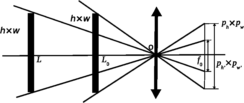
1.

Introduction

Infrared texture is an important feature in identifying scenery and has been used in various applications such as target detection, precision guidance, and three-dimensional scene simulation.^1–3 Infrared texture generation has been studied for decades, but because of security considerations, progress on the topic was seldom reported in the public literature.

The few published papers on infrared texture reveal the two methods used to generate infrared image texture: infrared texture simulation based on visible light texture^4–6 and the random field model.^7–10 The former method uses Planck’s equation to calculate the infrared radiation energy for each object in the scene and then the energy value is mapped using a specific gray level. The deviation of the specific gray level is computed by the variations of gray in the visible image. The final infrared image texture is obtained using the specific gray level and its deviation. This simulation method can be adapted for a large-scale scene that needs only a low amount of detail, but it is not suitable for a scene that requires a high amount of detail because the infrared and visible textures have different principles of formation. The other simulation method based on a random field model, e.g., long correlation models⁷ and the Markov random field model,^8–10 can generate infrared image texture. However, this method requires a large number of model parameter tests to determine the proper parameters, and this method is highly complex and has low fidelity.

To simulate infrared image texture at different distances, the simulated image is transformed by zooming in and out. The two simulation methods mentioned above do not take into consideration the attenuation of high frequency and the variation in the temperature difference of the scenery detail due to the atmospheric effect on transmission and different distances. The transformation of the simulated images obtained by the two methods discussed above is not reliable when the distance changes. Based on the image multiresolution pyramid principle, we propose an infrared image texture generation model based on scenery spatial frequency to generate infrared image texture at different distances. First, we calculate the scenery spatial frequency at a specific distance using the Nyquist frequency of the detector, and then we use the calculated scenery spatial frequency as the cut-off frequency to build a filter model based on distance. We use the filter to process the “zero”-distance infrared image texture captured by the thermal imager and downsample the filtered image. Second, given that the actual temperature difference corresponding to different scenery texture details will change with a change in distance due to the atmospheric transmission effect, we compare the changed temperature difference with the minimum resolvable temperature difference (MRTD) of the thermal image system. The comparative results are used to build a filter based on MRTD to decide whether the frequency should be recognized. Finally, after performing the above two steps of the filtering process, we obtain the final image texture.

Section 2 introduces the infrared image texture model based on scenery spatial frequency, Sec. 3 presents the experimental results and discussion, and Sec. 4 gives the conclusion of the paper.

2.

Thermal Infrared Image Texture Generation Model Based on Scenery Spatial Frequency

2.1.

Frequency Pyramid Principle of Imaging

An image pyramid is a series of images arranged in a pyramidal structure, which is effective in multiresolution image representation (Fig. 1). The size and resolution of the images gradually decrease from the bottom image to the top image of the pyramid. The size of the base layer $J$ (the original image) is $N\times N$ or $2^J\times 2^J$, where $J={\log }_{2}N$. The size of peak layer 0 is $1\times 1$, i.e., a single pixel. The size of a layer $j$ is $2^j\times 2^j$, where $0\le j\le J$. Therefore, a multiresolution pyramid is formed by starting with the $N\times N$ size of the original image and the image size of each successively smaller layer is an integral multiple of 2.

Fig. 1

Image pyramid.

In a photoelectric imaging system with a fixed number of pixels, when the distances change, the imaging process becomes a series of multiresolution displays. Therefore, the generation of infrared image textures at different distances is equivalent to the formation of an image pyramid: the “zero”-distance infrared image is the bottom image in the pyramid and has the highest resolution. The effects of distance and atmospheric transmission on the scenery infrared textures are equivalent to low-pass filtering and the process of downsampling in the image pyramid. A series of infrared image textures of different sizes and resolutions can be obtained by repeated filtering and downsampling. The filters are based on distance and MRTD. All of the filtering processes act on the “zero”-distance infrared image.

2.2.

Spatial Frequency Filter Based on Distance

The results of the scenery imaging on the detector are shown in Fig. 2, where $h$ and $w$ are the height and width of the scenery, O is the optic center, $f_0$ is the focal length of the infrared imaging system, and $p_h\times p_w$ and $p_{h^{\prime }}\times p_{w^{\prime }}$ are the image size at distance $L_0$ and $L$, respectively.

Fig. 2

Results of scenery imaging on the detector.

2.2.1.

Frequency filter model based on distance

For the infrared imaging system with a fixed number of pixels, the ability to distinguish scenery details decreases with increasing distance. The cut-off frequency $D_L$ is the frequency that the detector can distinguish at distance $L$. The cut-off frequency determines the level of detail of the scenery at $L$ and is calculated using $L$. Then a filter model based on the cut-off frequency is built and is used to process the “zero”-distance image. We call the filter a spatial frequency filter, denoted by $H_S$ and it is defined as

Eq. (1)

$$H_S=\{\begin{array}{cc}1,& f_L\le D_L\\ 0,& f_L>D_L\end{array},$$

where $f_L$ is the spatial frequency of the “zero”-distance image and $D_L$ is the cut-off frequency of the image at distance $L$.

We apply the Fourier transform $F(u,v)$ to the “zero”-distance image of size $M\times \mathrm{N}$:

Eq. (2)

$$F(u,v)=\sum _{x=0}^{M-1}\sum _{y=0}^{N-1}f(x,y)e^{-j2\pi (ux/M+vy/N)},$$

where $f(x,y)$ is the gray value at ($x,y$) on the “zero”-distance image. Then, the filtered image $G(u,v)$ in the frequency domain is calculated using the following equation:

Eq. (3)

$$G(u,v)=F(u,v)H_S(u,v).$$

The spatial-domain image $g_p(x,y)$ is obtained by using the inverse Fourier transform of $G(u,v)$ in the frequency domain:

Eq. (4)

$$g_p(x,y)=\{\text{real}[{\zeta }^{-1}[G(u,v)]]\}{(-1)}^{x+y},$$

where ${\zeta }^{-1}$ is the inverse Fourier transform.

The image size $(p_{h’}\times p_{w’})$ of the scenery at distance $L$ is determined by the relationship between the location of the scenery and the detector, as shown in Fig. 2. The $g_p(x,y)$ is filtered again using the downsampled window:

$$w=[\frac{p_{h^{\prime }}}{p_h}\times \mathrm{col}]\times [\frac{p_{w^{\prime }}}{p_w}\times \mathrm{row}],$$

where col and row are the number of columns and rows of the detector, respectively. We use $g_p(x^{\prime },y^{\prime })$ to denote the result of filtering $g_p(x,y)$. This filtered image is the simulated image when the detector is located at $L$ and the atmospheric transmission effect is not taken into consideration.

2.2.2.

Image cut-off spatial frequency based on distance

The horizontal and vertical sample frequencies, $f_w$ and $f_h$, respectively, of the detector are expressed as

Eq. (5)

$$f_w=1/(2\times d_w),$$

Eq. (6)

$$f_h=1/(2\times d_h),$$

where $d_w$ and $d_h$ are the width and height of the detector pixel. The imaging height ($p_{h’}$) and width ($p_{w^{\prime }}$) on the detector at $L$ are expressed as

Eq. (7)

$$p_{h^{\prime }}=h\times f_0/L,$$

Eq. (8)

$$p_{w^{\prime }}=w\times f_0/L,$$

where $f_0$ is the focal length of the infrared imaging system and $h$ and $w$ are the height and width of the scenery. The cut-off spatial frequencies of the image at $L$ are determined by the relationship between the scenery and the detector and are defined as follows:

Eq. (9)

$$D_{Lh}=p_{h^{\prime }}/h_{\text{dect}}\times f_h,$$

Eq. (10)

$$D_{Lw}=p_{w^{\prime }}/w_{\text{dect}}\times f_w,$$

where $D_{Lh}$ and $D_{Lw}$ are the vertical and horizontal cut-off spatial frequencies of the image at $L$ and $h_{\text{dect}}$ and $w_{\text{dect}}$ are the height and width of the image on the detector plane.

3.

Experimental Results and Discussion

We simulated the infrared image texture of scenery at different distances based on the “zero”-distance image. The “zero”-distance image was captured by the VarioCAMLong Wave Thermal Imaging System (InfraTec GmbH, Dresden, Germany). The parameters were as follows: $\text{resolution}=240\times 320\text{pixels}$, wave $\text{band}=7.5$ to $14\mu \mathrm{m}$, temperature detection $\text{range}=-40$ to 1200°C, $\mathrm{NETD}=0.08°\mathrm{C}$, ${\mathrm{SNR}}_T=2.8$, $f_p=50\mathrm{Hz}$, $t_e=0.2\mathrm{s}$, ${\tau }_d=1/f_p$, and $\mathrm{\Delta }f=\pi /(4*{\tau }_d)$.

Two “zero”-distance images were collected on October 18, 2013, and were shown in Figs. 3(a) and 3(b). They were taken at 40 deg north latitude under a cloudy sky. In addition, there was haze that made visibility 0.5 km, and the atmospheric transmissivity was $<0.7$. Using the model of the relationship between the frequency distribution and the temperature difference of the scenery, we calculated five typical points of frequency and their corresponding average temperature differences. The fitting curves of the relationship are shown in Figs. 3(c) and 3(d). The coefficients of Eq. (21) for the curves in Figs. 3(c) and 3(d) are as follows: $a_1=0.1766$, $b_1=-0.8286$, $c_1=0.176$, $d_1=-0.03884$; $a_2=1.816$, $b_2=-0.6038$, $c_2=1.118$, $d_2=0.03606$.

Fig. 3

(a) and (b) Two “zero”-distance infrared images and (c) and (d) the fitting curves of the relationship between the frequency and the average temperature difference for the images in (a) and (b), respectively.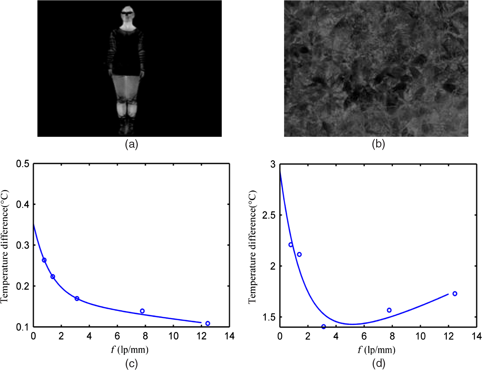

The infrared image textures shown in Fig. 4(a) were simulated as follows. First, we determined the distance of the simulated image; we assumed that it was 5 m. Second, we applied the spatial frequency filter based on distance and downsampled the “zero”-distance infrared image [Fig. 4(a)] using Eq. (3); the experimental results are shown in Figs. 4(b) and 4(c) in frequency and spatial domains, respectively. Finally, we used the infrared texture image filter based on MRTD from Eq. (14) to process the filtered image shown in Fig. 4(c); the result is shown in Figs. 4(d) and 4(e).

Fig. 4

Infrared image texture generation procedure based on a “zero”-distance infrared image at 5 m. (a) “Zero”-distance infrared image, (b) result of filter in frequency domain based on distance, (c) result of filter in spatial-domain based on distance, (d) result of filter in frequency domain based on MRTD, and (e) result of filter in spatial-domain based on MRTD.

We found that the image in Fig. 4(c) is fuzzier and smaller than that in Fig. 4(a), and the image in Fig. 4(e) is fuzzier than that in Fig. 4(c). Some details are attenuated because of the atmospheric transmission effect.

Figure 5 compares the simulated image with the infrared image captured by the thermal imager (real infrared image) when the subject was 5 m from the imager. To compare the two images directly and analyze the simulation, the simulated image was extended to the whole field of view. Both images [Figs. 5(a) and 5(b)] are relatively similar from a subjective point of view. The slight discrepancy between the two [Fig. 5(c)] is caused mainly by the nonconformity of scenery locations in the two images. The location of the object in the infrared image is not always just centered in the entire field of view, so in the simulation image, the nonconformity is caused.

Fig. 5

Comparison of (a) the image at 5 m captured by the thermal imager, (b) the simulated image, and (c) image showing the discrepancy between (a) and (b).

Figure 6 shows the histograms¹⁴ of the infrared image captured by the thermal imager [Fig. 5(a)] and the simulated image [Fig. 5(b)]. Figures 6(a) and 6(b) are the whole histograms and Figs. 6(c) and 6(d) are the histograms in the gray-level range of 0 to 100 for the infrared image and the simulated image, respectively. The histograms in Figs. 6(a) and 6(b) have a peak value between 0 and 255 gray levels. The histograms in Figs. 6(c) and 6(d) show that the infrared image and the simulated image have similar distributions of gray levels.

Fig. 6

(a) Whole histogram of image captured by the thermal imager. (b) Whole histogram of simulated image. (c) Histogram in the gray-level range of 0 to 100 for image captured by the thermal imager. (d) Histogram in the gray-level range of 0 to 100 for the simulated image.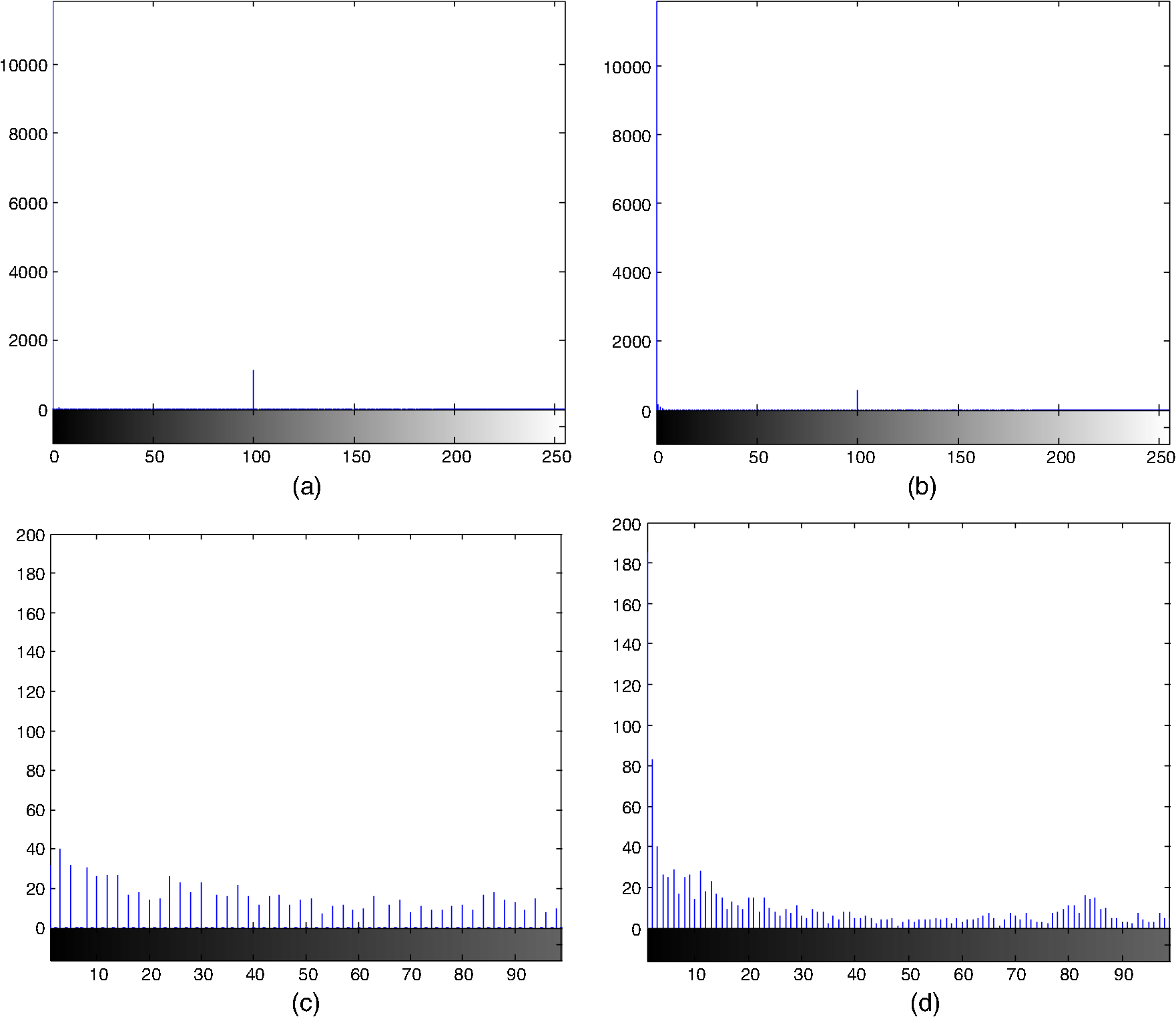

The simulated images and real infrared images at 10, 15, and 20 m are presented in Fig. 7. The details of the simulated images and the real infrared images decrease with increasing imaging distance. The simulated image has a texture similar to that of the real infrared image when the imaging distances of the two images are the same.

Fig. 7

Comparison of real (top panels) and simulated (bottom panels) images at distance (a) and (d) 10 m, (b) and (e) 15 m, and (c) and (f) 20 m.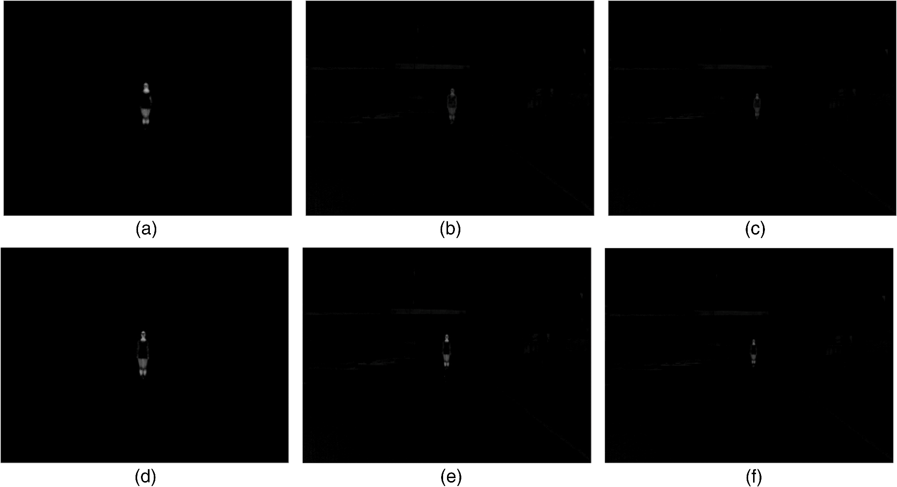

Figure 8 presents the real infrared image [Fig. 3(b)] and the simulated images of the grass at different distances. The “zero”-distance captured image [Fig. 8(a)] is of a patch of grass 0.6-m wide and 0.45-m high. We used the proposed filter model to process the “zero”-distance infrared image at different distances to obtain the simulated infrared texture images. The simulated images should be the entire field of view, so the texture-matching technology based on the sample plot is adapted to each simulated image; the simulated results are shown in Figs. 8(b)–8(f). The figures show that as the distance increased, the details gradually became blurrier. These changes reflect the variations in the details of the scenery infrared texture at different distances.

Fig. 8

(a) The “zero”-distance infrared image captured by the thermal imager. (b)–(f) The simulated images of the grass scenery at 1, 2, 3, 5, and 10 m.

Mean square error (MSE) and peak signal-to-noise ratio (PSNR) are often used as the evaluation indices¹⁵ to compare the similarity of two images. In general, if the $\mathrm{PSNR}>20$, there is a strong similarity between the two images.¹⁵ The similarity indices of the captured images and simulated images at different distances are presented in Table 1.

Table 1

Indices used to evaluate the similarity of the captured images and the simulated images at different distances.

The results in Table 1 show that when the distance increases, the MSE decreases and the PSNR increases, indicating that the similarities increase as the distance increases. All the PSNR values in this study were greater than 20, so the captured image and simulated images are very similar when the distance is between 5 and 20 m. The small MSE values and the large PSNR values in Table 1 suggest that the proposed filter model has high fidelity and is valid.

This study has one limitation, i.e., the proposed model was tested on only two thermal images, that of the person and the grass. However, we limited the number of images for three reasons. First, the performance of the model in simulating scenery depends on the imaging distance and viewing direction, not on the object in the scenery. Second, the experimental images of the person and the grass show the degradation of the image and the variation in the texture detail that occur when the imaging distance changes. We verified with the two experimental images that the proposed model is valid for the scenery simulation in which the “zero”-distance infrared image of the scenery is obtained by the perpendicular shoot to the scenery (i.e., the grass was shot from above, whereas the person was shot horizontally), but it is not valid for the scenery simulated from different viewing directions. Therefore, we did not use more images to test the model from the vertical direction to the scenery. Third, experimental conditions that were more complex and more materials would have been necessary to capture additional thermal infrared images at different viewing directions and distances, e.g., we may have had to use unmanned drones. Therefore, when the experimental conditions are appropriate, we will consider capturing more images for our future work.

4.

Conclusion

Based on the principle of the multiresolution image pyramid, we proposed a new thermal infrared image texture generation model based on scenery spatial frequency. The model was based on a “zero”-distance infrared image. Two typical sceneries were simulated using the model, and the simulations were compared with the infrared image texture captured by a thermal imager. The experimental results validated the proposed model by showing that it can reflect the features of infrared image texture and the imaging principle at different distances. In conclusion, the proposed model is able to effectively simulate infrared images with textures on the large-scale background and can meet some of the requirements of qualitative analysis. In the future, we will capture and simulate sceneries from different directions and distances and use them to improve the robustness of the proposed model.