|
|
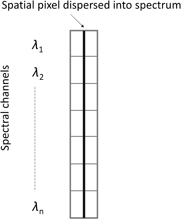
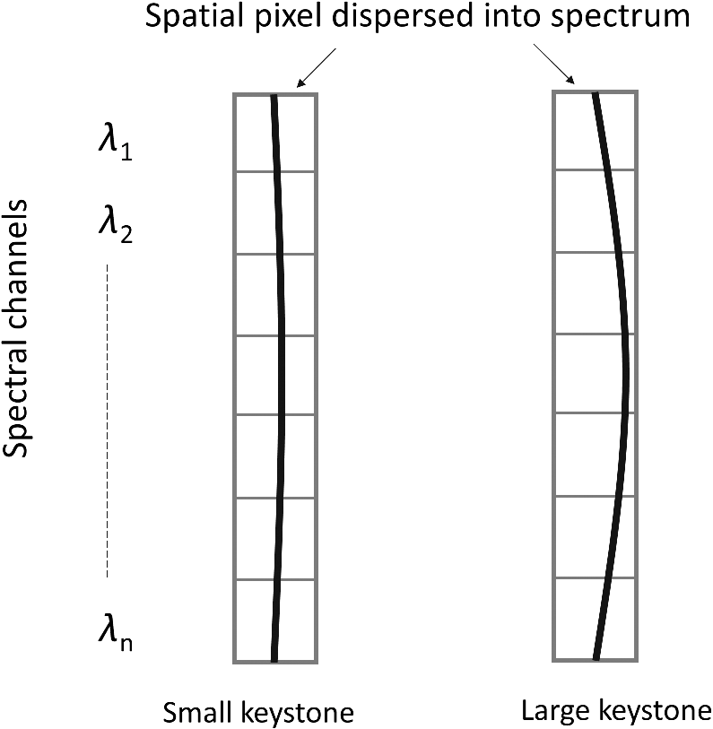
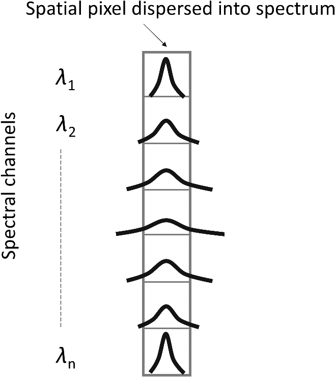
1.IntroductionHyperspectral cameras—also called imaging spectrometers—are increasingly used for various military, scientific, and commercial purposes. Important criteria for the image quality of such cameras are image sharpness as well as good spatial and spectral coregistration. Spatial misregistration, caused by keystone and variations in the point spread function (PSF) across the spectral channels, distorts the captured spectra.1 A similar error occurs in the spectral direction (spectral misregistration, caused by the smile effect and corresponding PSF variation). Quantifying these errors, as well as the image sharpness, would allow for evaluation and comparison of the performance of different hyperspectral imagers. However, how to measure and quantify these errors is currently not well defined. Usually, the two factors that cause spatial misregistration, keystone and the corresponding PSF, are addressed separately. The same is done for smile and the corresponding PSF. In Ref. 2, the authors measured keystone in their Offner camera by imaging a polychromatic point source at various positions along the slit. Smile was measured similarly by the use of various spectral lamps at specified wavelengths. The authors made certain assumptions about the shape of the keystone and smile in the camera in order to achieve their results. Keystone measurements, performed as described in Ref. 2, are very sensitive to the position of the point source relative to the pixel center, and some of the later methods address this issue by repeating the point source measurements at several positions within each characterized pixel. More recently, the German Aerospace Center (DLR) performed a thorough laboratory characterization of two hyperspectral cameras:3,4 NEO HySpex VNIR-1600 and SWIR-320m-e. The characterization included measurements of keystone, smile and the full width at half maximum (FWHM) of the corresponding PSFs. In order to ensure high accuracy of the results, the keystone measurements were done for several point source positions within each characterized pixel. A different approach for measuring keystone, smile, and the spatial and spectral response functions is proposed in Ref. 5. There, the authors suggest the use of a set of affordable reference objects for the measurements in order to simplify the hardware necessary for camera characterization. Keystone and spatial response functions are measured with a set of black and white bars that are located relatively close to the camera. This location of the test objects makes the method less suitable for characterization of cameras that are corrected for long distances, which includes all airborne and many field cameras. In order to reconstruct all the parameters from a sparse measurement matrix, various assumptions about the image geometry are made, and it is also necessary to interpolate the data. The obtained results have been used to reduce misregistration in hyperspectral data in postprocessing by the use of deconvolution.6 The authors indicate that the accuracy of their method in its current implementation may be close to 0.1 pixels for the keystone measurements.5 However, keystone has to be characterized significantly more precisely than that in order to take full advantage of a good resampling technique for keystone correction in postprocessing.7 Also, residual keystone in good existing cameras is often .4 Therefore, the current implementation of this method may not be suitable for high-end cameras, although the achieved precision is impressive considering the simplicity of the setup. Keystone and smile measurements, as well as measurements of spatial and spectral PSF, provide invaluable feedback during alignment and focusing of hyperspectral cameras. However, it has been shown that keystone and smile, when considered independently from the corresponding PSFs, do not adequately describe coregistration errors.1 References 8 and 9 describe a method for characterizing spatial and spectral coregistration errors that combines keystone and smile with their corresponding PSFs into the spatial and spectral response functions. However, this approach does not accurately predict the maximum possible errors in the case of bright subpixel sized objects on a dark background. Also, this method is not sensitive to image sharpness and the effect it has on co-registration. Image sharpness is an important parameter to consider when quantifying the image quality of a hyperspectral camera. Previous papers1–9 do not discuss the fact that a higher image sharpness (i.e., narrow PSFs) increases the errors caused by keystone and PSF variations in the acquired data. Existing criteria for quantifying image sharpness, such as PSF and modulation transfer function (MTF), are adapted for traditional imaging systems,10 and it is not clear how to apply these methods to hyperspectral cameras where different wavelengths are channeled to different parts of the imaging sensor. We wanted to find a method for quantifying the image quality of hyperspectral cameras that is intuitive, easy to implement, and not based on any prior assumptions about the nature of the errors or the scene, while at the same time providing a reliable and accurate way to compare the performance of different hyperspectral imagers. The method we suggest in this paper fulfills these requirements and is based on a very basic principle: simply determine “how much of the energy collected by the hyperspectral camera ends up in the correct pixel in the final data cube.” When this is known, image sharpness and spatial and spectral misregistration can easily be determined. These three parameters are particularly suitable for assessing camera performance in terms of output data quality and could be a valuable tool for camera manufacturers during the final stage of production for verifying the success of focus and alignment efforts. The same three parameters could also be a very convenient tool for camera users when they are choosing an instrument for their application. In this paper, we will mainly focus on spatial misregistration and image sharpness in the across-track direction. The necessary measurements can then be obtained by moving a point source in subpixel steps along the pixel array in the across-track direction. This means that the method is easy to implement and only requires equipment that is normally already present in an optical lab (collimator with a point source and a high-resolution rotation or translation stage). For spectral misregistration caused by smile and corresponding PSF variations, similar measurements could be performed with the use of a spectrally tuneable monochromatic light source. We will explain the idea behind the method in more detail in Sec. 2, whereas the mathematical framework will be presented in Sec. 3. Section 4 describes the measurement procedure in detail. In Sec. 5, we quantify the performance of two HySpex SWIR 384 cameras using the suggested method. In Sec. 6, we briefly discuss how the method can be expanded for measuring spectral misregistration. The conclusions are given in Sec. 7. 2.MethodWe will explain the nature of keystone and PSF variations in a hyperspectral camera and how the combined effect of these two error sources, i.e., spatial misregistration, can be measured in a simple and straightforward way. We will also explain what is meant by image sharpness, how the sharpness affects the errors caused by keystone and PSF variations, and how we suggest that this parameter be measured and quantified for a hyperspectral camera. 2.1.Keystone and PSF VariationsConsider a polychromatic point source that is captured by a hyperspectral camera and dispersed in the vertical direction. In the ideal case, the image of the point source would be a straight vertical line (see Fig. 1). However, two things will happen in an optical system:
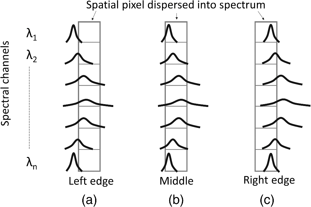
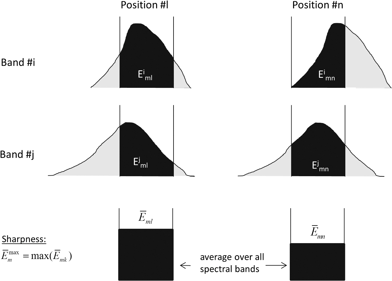
2.2.MisregistrationLet us now consider a camera where both keystone and differences in PSF for different spectral channels are present. The image of the point source in different spectral channels may then look as shown in Fig. 4(a). Let the total energy in each spectral channel be normalized, i.e., set to have the value 1. The “true” spectrum for the point source will then be a straight line, as shown in Fig. 4(b) (dashed line). However, due to keystone and PSF variations, the captured spectrum [solid line in Fig. 4(b)] will deviate from the true spectrum by an amount that will differ for different spectral channels. This deviation can be used as a measure of misregistration and will include the effects from both keystone and PSF variations. For each spectral channel, for a given point source position in a given spatial pixel, the misregistration can then be calculated as the difference between the energy collected in that spatial pixel for that spectral channel and the mean energy for the corresponding pixel column. The misregistration should be given as a fraction of the mean energy, since it is the energy difference relative to the mean energy that decides how erroneous the resulting spectra will be. The misregistration may vary considerably for different point source positions within a spatial pixel. However, by measuring the misregistration across spectral channels for several different point source positions, the standard deviation (across spectral channels and point source positions within one spatial pixel) can be calculated and used as a measure of typical misregistration for that spatial pixel. The process can be repeated for all spatial pixels across the field of view (FOV). Fig. 4Combined effect of keystone and point spread function (PSF) variations on (a) the image of the point source and (b) the captured spectrum.  The pixel column that contains the largest part of the energy for a given point source position is defined as the spatial pixel where the point source is located. One could argue that the errors in the spectrum (relative to the signal level) are even larger in the neighboring pixels, and that perhaps those pixels should be used to quantify the misregistration instead. However, there are several reasons why we do not recommend this. The signal levels in the areas of the PSFs that extend into the neighboring pixels are typically low, and it may be quite difficult technically to measure them precisely enough. Further, the measurement of the misregistration may become very sensitive to the step length between the point source positions, since a small change in point source position may give a large relative change in the signal level at the low signal levels in the neighboring pixels. Also, for sharp cameras, the neighboring pixels may have zero signal level, i.e., only noise will be recorded for one or more point source positions. Finally, and most importantly, the underlying cause for the misregistration (keystone and PSF variations) is the same for both the spatial pixel that captures the point source and the neighboring pixels. The misregistration of one camera relative to another should, therefore, be reflected similarly in both cases. However, the misregistration can be measured more consistently and much more precisely if the pixel column where the point source is located, i.e., the pixel column that captures most of the energy, is used. Note that the method for measuring misregistration presented here does not rely on any assumptions regarding the shapes of keystone curves or PSFs. Also, the method does not assume a particular light sensitivity distribution within a single sensor pixel. With existing relatively low cost equipment, misregistration measurements can be performed sufficiently accurately that the effects of keystone that are significantly smaller than 0.1 pixels can be detected and quantified, making the method suitable for high-end cameras. 2.3.SharpnessImage sharpness is a very important parameter to consider when discussing misregistration of hyperspectral cameras. The reason for this is that, in principle, one could build a hyperspectral camera that would give such a blurry image that even a relatively large keystone would give only a very small misregistration. Figure 5(a) shows the image of a point source across spectral channels for both a sharp camera (left) and a very blurry camera (right). Both cameras have the same keystone (indicated by the dashed line). The spectra captured by each of the cameras are shown in Fig. 5(b), together with the corresponding true spectra. Clearly, the blurry camera has a much lower misregistration than the sharp camera. However, this is achieved by strong blurring of the image. The blurry camera will give spectra that are closer to the real spectra present in the scene, but the “imaging” aspect of such an imaging spectrometer—in terms of spatial resolution—is clearly compromised. The most extreme example would be a camera that gives so blurry image that it is not able to resolve any spatial details within its FOV. At the same time, this camera would most likely have very low misregistration. Fig. 5Comparison of the camera performance in terms of misregistration—or errors in the captured spectrum—for a sharp camera (left) and a very blurry camera (right), illustrating the importance of also considering the image sharpness when discussing misregistration in hyperspectral cameras. (a) The image of a point source across spectral channels for the two cameras, and (b) the corresponding true and captured spectra. 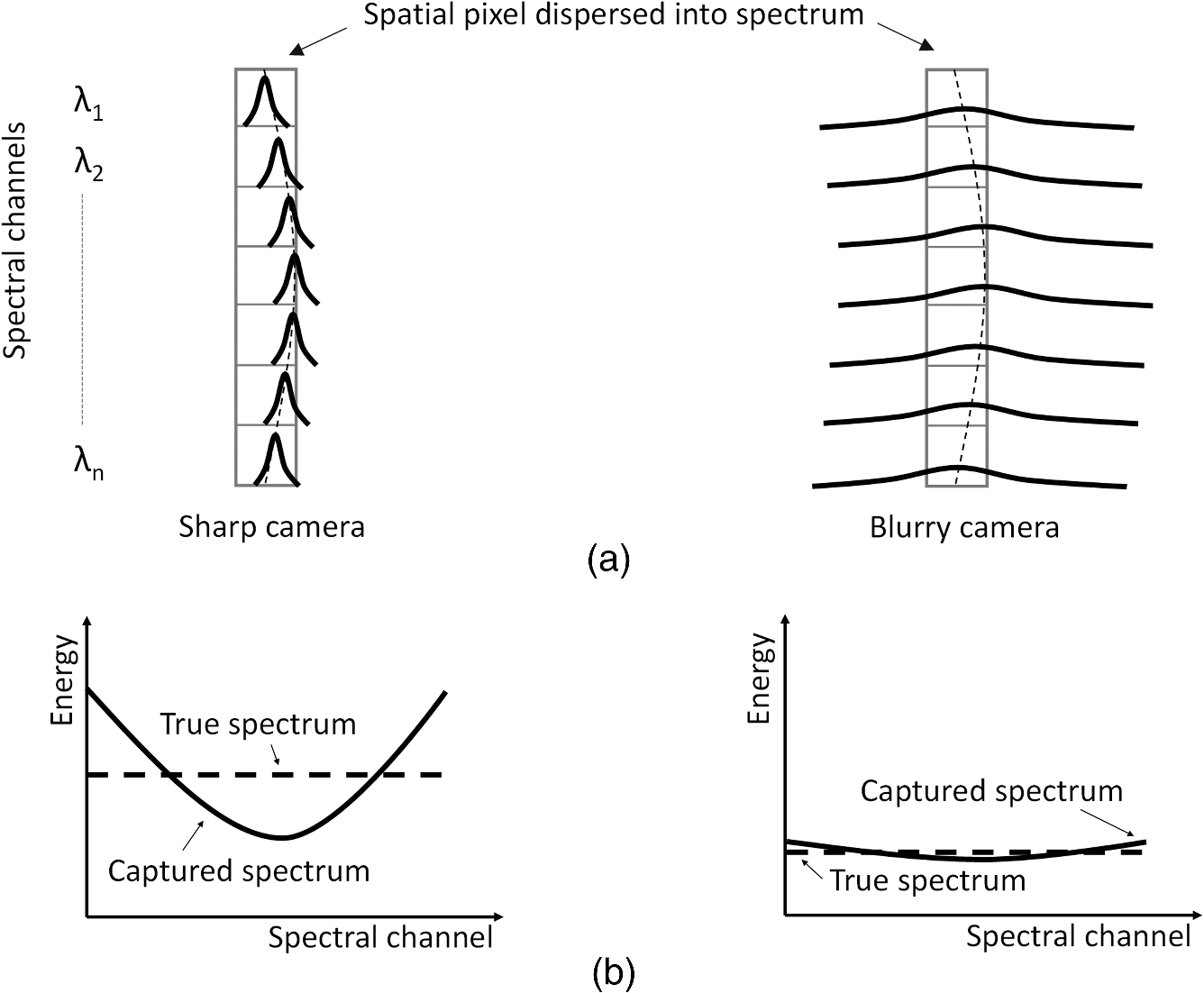 For traditional imaging systems, such as photographic lenses, image sharpness is expressed in terms of PSF or the combination of MTF and phase transfer function.10 In principle, these methods could be used for hyperspectral cameras, too. However, since in push-broom hyperspectral cameras (and most other hyperspectral camera types), the optics direct different wavelengths to different parts of the imaging sensor, significant modifications of these methods would be necessary in order to adequately express camera performance. Here, we suggest a different approach which is well suited for evaluating the sharpness of a hyperspectral camera. Conveniently, this method utilizes the same data that is acquired for measuring misregistration. The method is intuitive and could easily be modified if required by a specific application. Let us take a look at how the sharpness of a single spatial pixel could be expressed based on point source measurements made at different spatial positions within the pixel. The total energy in each spectral channel is normalized as before. As the point source is moved from one side of the spatial pixel to the other, the mean energy (taken over all spectral bands) captured by the pixel column will vary, see Fig. 6. Typically, the mean energy will be lower close to the edges of the spatial pixel [Figs. 6(a) and 6(c)] and higher in the middle [Fig. 6(b)]. The maximum mean energy (among all point source positions) captured within the pixel column could be used as a measure of sharpness for that spatial pixel. For a very sharp camera with a small keystone, where practically all the energy in all spectral channels falls within the correct pixel column, the sharpness is close to 1. For more blurry cameras, or cameras where the keystone is large, the sharpness is smaller than 1. Note that the suggested method for quantifying sharpness takes into account the loss of image sharpness that occurs in hyperspectral cameras due to the keystone. If the keystone is large, the image of a point source across the spectral channels will be distributed over more than one spatial pixel, even if the camera is very sharp in every individual spectral channel according to traditional criteria such as PSF width and MTF. 3.Mathematical FrameworkWe will now describe the mathematical framework for the method. The measurements are performed by moving a point source in subpixel steps along the pixel array in the across-track direction. The point source positions within one pixel should be equally spaced and sufficiently dense: typically, a few tens of positions per pixel. The normalized energy for spatial pixel in spectral band when the point source is at position is given by where is the corresponding measured energy content of spatial pixel in spectral band when the point source is at position , and is the total number of spatial pixels. Note that the term “pixel” may refer here to a pixel in the final data cube or to a sensor pixel, depending on the type of camera being measured. For hyperspectral cameras where the keystone is corrected in postprocessing, such as resampling7 and mixel cameras,11 the final data cube should be used as the basis for the calculations. For traditional cameras where the keystone is corrected to a fraction of a pixel in hardware, the pixels in the final data cube are equivalent to the sensor pixels, and the calculations can be performed directly on the recorded sensor pixel values. The sum over all pixels in spectral band is thenThis is illustrated in Fig. 7. Note that in a real camera, noise will be present. For this reason, only a few spatial pixels on each side of the point source should be included when calculating the sums in Eqs. (1) and (2), rather than using all spatial pixels for the calculations. Also, it is important to have a high signal-to-noise ratio in the measurements. Fig. 7The upper figure shows the PSF for a point source at position in spectral band distributed over four spatial pixels. The measured energy in pixel is , with corresponding normalized energy shown in the lower figure. 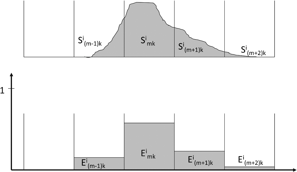 The mean value for the normalized energy over all spectral bands for spatial pixel when the point source is at position is given by where is the total number of spectral bands.The point source is defined to be in spatial pixel when the mean value for the normalized energy in the corresponding pixel column is larger than in any of the other pixel columns. This means that the point source is in pixel for all positions where Here, is the total number of such positions for pixel . The point source positions corresponding to pixel will typically follow each other consecutively, but this is not a requirement for the method to work. In principle, one might have a point source position corresponding to a neighboring pixel mixed in between. For instance, this could happen if the PSF has a large dip in the middle. However, normally the FWHM of a camera’s PSF is comparable to its pixel size, so that this situation will not occur regardless of the shape of the PSF. Figure 8 shows an example of different point source positions for a given pixel in one spectral channel. Fig. 8Different point source positions for pixel in one spectral channel. The point source is moved in small equally spaced subpixel steps from left to right. In the bottom, the point source has moved to pixel . 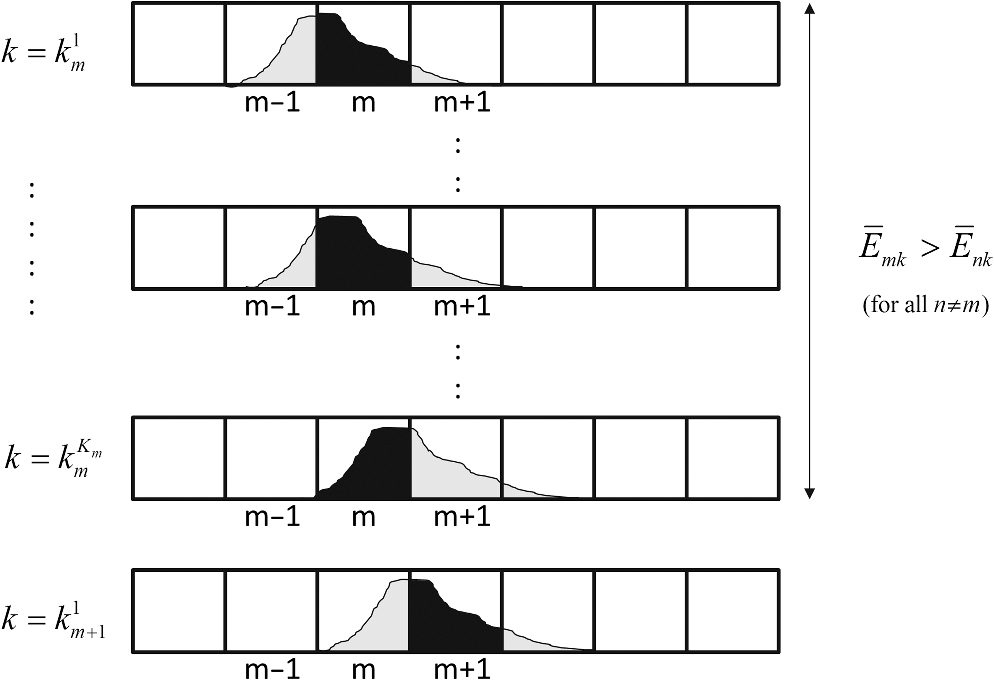 3.1.SharpnessThe sharpness is quantified as the maximum fraction of the total energy that a spatial pixel can contain and has a value in the range [, 1]. The lower limit corresponds to an even distribution of the energy over all pixels, whereas the upper limit corresponds to all the energy being contained within one single pixel. The sharpness at spatial pixel can be found from where is given by Eq. (3). Figure 9 shows examples of the PSF for pixel in different bands and different point source positions and illustrates the sharpness for the pixel.3.2.Misregistration—Standard DeviationMisregistration is quantified as the relative difference between the energy recorded in a pixel and the mean energy over all spectral bands for that spatial pixel. The misregistration for pixel in spectral band when the point source is at position is given by: The standard deviation for the misregistration for spatial pixel when the point source is at position can then be calculated from Finally, the mean standard deviation for the misregistration for spatial pixel , taken over all point source positions corresponding to that spatial pixel, can be found from where is the total number of point source positions for pixel .3.3.Maximum MisregistrationWhile calculating the standard deviation of the misregistration gives a good measure of the typical size of the misregistration, it is sometimes important to also be aware of occurrences of untypically large misregistration. These are normally hidden in the standard deviation. For this reason, we will also calculate the maximum misregistration for each spatial pixel. The minimum normalized energy over all spectral bands at spatial pixel when the point source is at position is while the maximum normalized energy over all spectral bands at spatial pixel when the point source is at position isThe maximum misregistration for spatial pixel when the point source is at position is then given by Finally, the maximum misregistration for spatial pixel (over all point source positions) can be found from The maximum misregistration is illustrated in Fig. 10. Fig. 10Illustration of maximum misregistration for pixel . For each of the two point source positions in the figure, the PSFs of the two spectral channels with the largest difference in normalized energy are shown. This is the situation where the misregistration is the largest for that point source position. As shown here, the pair of spectral channels that gives the largest misregistration may be different for different point source positions. The maximum misregistration for the pixel is defined to be the largest maximum misregistration over all point source positions for that pixel. 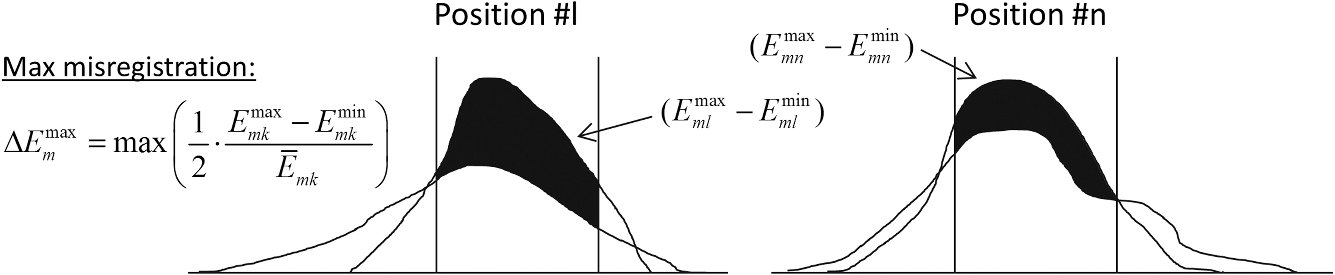 3.4.Probability of Misregistration Being Larger Than a Given ThresholdThe maximum misregistration may, in some cases, be very large. If the misregistration is above a certain threshold so that the spectrum becomes so distorted that it is no longer useable, then it does not matter how much larger than the threshold the misregistration is. Instead, it may then be useful to look at how many occurrences there are of the misregistration being larger than the threshold.7 For this reason, we introduce the parameter that describes the probability of the misregistration being larger than a given threshold for spatial pixel : where is the total number of point source positions for pixel and is given byHere, is the maximum misregistration for spatial pixel when the point source is at position . 4.Measurement ProcedureThe measurement procedure for quantifying spatial misregistration and image sharpness is as follows:
5.Experimental Setup and ResultsWe have tested two HySpex SWIR 384 cameras, a prototype and a production-standard camera, with the method proposed in this paper. The cameras were manufactured by Norsk Elektro Optikk AS and have the following main specifications:
A typical experimental setup, which was also used in this case, is shown in Fig. 11 and consists of a point source (1), a parabolic mirror (2) which projects the point source to infinity, and (3) a high-resolution rotation stage. The push-broom hyperspectral camera (4) to be tested is mounted on the rotation stage and rotated as indicated by the arrows in the figure. The across-track FOV of the hyperspectral camera is in the vertical direction. Fig. 11The experimental setup consisting of a point source (1), a parabolic mirror (2) which projects the point source to infinity, and a high-resolution rotation stage (3). The push-broom hyperspectral camera (4) to be tested is mounted on the rotation stage and rotated as indicated by the arrows. 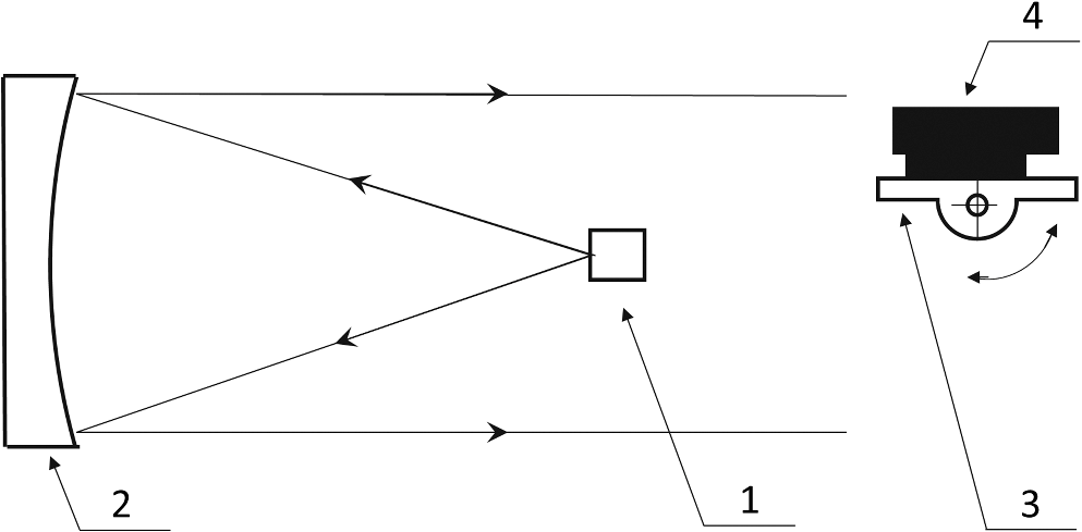 As usual for such a set-up, a polychromatic point source was used.2–4 A polychromatic point source makes it possible to simultaneously measure spatial misregistration in all spectral channels. This reduces the measurement time considerably compared to using several monochromatic point sources, and data from all spectral channels, not only a few selected, will contribute to the calculated misregistration. The latter is important because both the keystone and PSF may change quite rapidly as a function of wavelength.3 Since, in this type of camera, both sharpness and misregistration are parameters that change quite slowly as a function of FOV, we decided that it would be sufficient to perform measurements for only approximately every 10th spatial pixel. In each spatial position where the measurement was performed, the image of the point source was moved across a distance equivalent to about 3 pixels in order to make sure that at least 1 pixel was properly covered by the measurements. The camera was rotated so that the image of the point source was moved in steps of , i.e., about 100 measurements were performed inside one pixel. Note that if the tested camera has very high spatial resolution, it may be better to use the rotation stage (3) only for coarse positioning of the point source within the camera’s FOV and then move the point source (1) itself in small steps inside the pixel of interest. In addition, 200 measurements were made of the background. The average of the background measurements was subtracted from each of the point source measurements. Sharpness as well as mean standard deviation for the misregistration and maximum misregistration was calculated according to the method described in Sec. 3. A window of 11 spatial pixels around the point source (i.e., five spatial pixels on each side) was used for the calculations. The values for the spatial pixels where measurements were not performed were linearly interpolated. Figure 12 shows the results for the HySpex SWIR 384 prototype camera. Figure 13 shows the results for the production-standard HySpex SWIR 384 camera. Fig. 12The test results for the HySpex SWIR 384 prototype camera. The blue curve shows the sharpness as a function of spatial pixel number, whereas the green curve shows the mean standard deviation for the misregistration and the red curve shows the maximum misregistration. 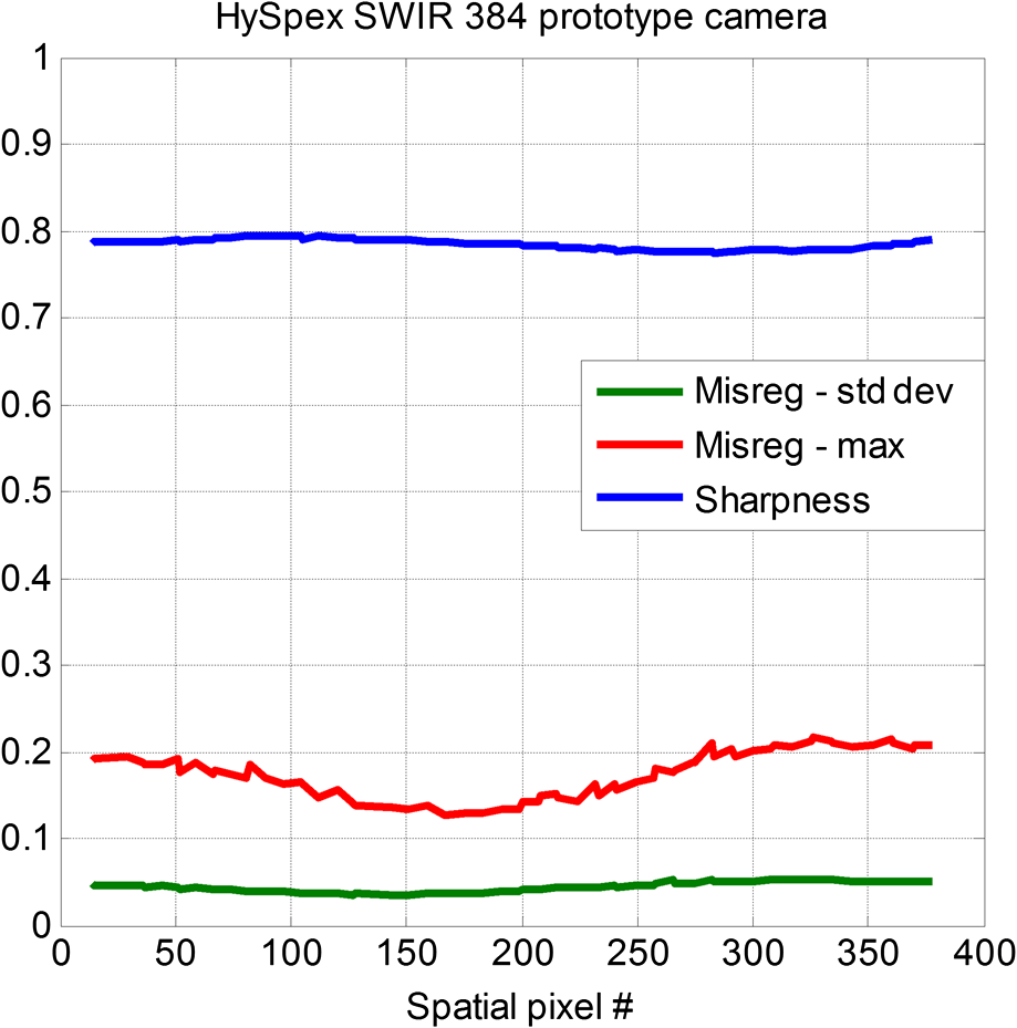 Fig. 13The test results for the production-standard HySpex SWIR 384 camera. The blue curve shows the sharpness as a function of spatial pixel number, whereas the green curve shows the mean standard deviation for the misregistration and the red curve shows the maximum misregistration. 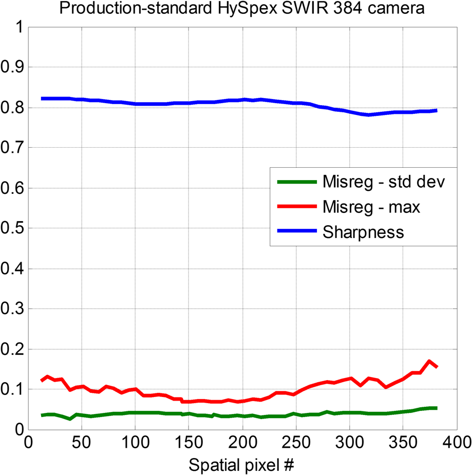 The form of data representation used in Figs. 12 and 13 is very useful for assessing the quality of a camera. For the tested HySpex SWIR 384 prototype camera (Fig. 12), the graphs indicate reasonably consistent sharpness across the FOV and a moderate misregistration increase at the edges of the FOV compared to the center. This is what should be expected from a camera of this type when it is aligned reasonably well. One of the strengths of the suggested method is the graphic representation of the results that makes comparison between two different cameras simple and intuitive. By direct comparison between Figs. 12 and 13, we can now easily determine which of the two tested cameras gives the best performance. We see that the production-standard HySpex SWIR 384 camera (Fig. 13) has noticeably lower maximum spatial misregistration (red curve) than the prototype. The mean standard deviation of the misregistration (green curve) as well as the sharpness (blue curve) is also somewhat better compared to the prototype. The production-standard camera should, therefore, acquire more accurate data than the prototype: the errors in the acquired spectra will be lower and this is not achieved at the expense of sharpness—the sharpness is actually marginally better in the production-standard camera compared to the prototype. Note that the misregistration, shown in Figs. 12 and 13, is not equivalent to keystone, i.e., a misregistration of 0.05 does not mean that the keystone is 0.05 pixel. There is a fundamental difference between keystone and misregistration: two cameras that both have the same keystone will have different misregistration if their sharpness is different. The keystone of a camera is not affected by image sharpness, but the errors caused by a given keystone (for a given scene) will depend on the sharpness of the camera7 in the same way as misregistration does. Therefore, misregistration (as defined here) seems to be a much better predictor for the errors that can be expected, and also a more suitable measure for the camera performance, than keystone. Also, the effect of both keystone and PSF variations as a function of wavelength is taken into account in the presented misregistration curves. For the cameras tested here, the keystone was corrected as well as possible in the hardware during design, and the misregistration and sharpness calculations could, therefore, be performed directly on the recorded sensor pixel values. Note, however, that if a camera where the keystone is corrected in hardware has a residual keystone that is larger than 0.5 pixel for some sensor pixels, then it is possible to reduce the keystone so that it becomes smaller than 0.5 pixel everywhere by replacing such a pixel with the correct neighboring pixel (nearest neighbor resampling). The misregistration and sharpness calculations should then be performed on the final data cube instead, after the necessary pixel replacements have been made. Similarly, the method could be used for resampling cameras7 and mixel cameras11 by performing the misregistration and sharpness calculations on the final data cube, after resampling or restoring of the data has been performed. 6.Measuring Spectral Sharpness and Spectral MisregistrationThe method can easily be expanded to also quantify spectral misregistration of a hyperspectral camera. When measuring spatial misregistration, we move a broadband point source across the FOV. When measuring spectral misregistration, we will have to point the tested camera at a large and (nearly) monochromatic light source instead and then scan the central wavelength of the monochromatic light source across the entire wavelength range of the camera. The setup for measuring spectral misregistration is shown in Fig. 14. A tested hyperspectral camera (3) is mounted in front of an integrating sphere (2). The sphere (2) is filled with monochromatic light by a tuneable laser (1) or another type of nearly monochromatic tuneable light source. During the measurements, the wavelength of the light source is changing in small steps to cover the entire wavelength range of the tested camera. Each step should be several times smaller than the spectral resolution of the camera. Fig. 14The experimental setup for measuring spectral misregistration, consisting of a tuneable laser (1) and an integrating sphere (2) which fills the FOV of the push-broom hyperspectral camera to be tested (3) with monochromatic light. 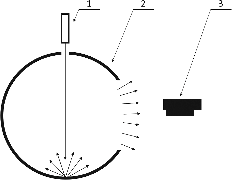 The measurement procedure and the following calculations will be equivalent to those for measuring spatial misregistration. Details of the mathematical framework and the measurement procedure can be derived from Secs. 3 and 4, respectively. The graphs which describe camera sharpness in the spectral direction, as well as a camera’s spectral misregistration, can be generated similarly to Figs. 12 and 13. Both parameters should be plotted as a function of wavelength. 7.ConclusionsWe have proposed a method for measuring and quantifying image quality in push-broom hyperspectral cameras in terms of spatial misregistration caused by keystone and variations in the PSF across spectral channels, and image sharpness. The method is easy to implement and requires only equipment that is normally already present in an optical lab (collimator with a point source and a high-resolution rotation or translation stage). The measurements are performed by moving a point source in subpixel steps along the pixel array in the across-track direction. The calculations are performed on the final data cube, making the method equally suitable for both traditional push-broom hyperspectral cameras where keystone is corrected in hardware, as well as resampling and mixel cameras where keystone is corrected in postprocessing. The method does not require any assumptions regarding the shape of keystone curves, shape of the PSFs, or light sensitivity distribution inside a single sensor pixel. Further, the method is able to measure the effects of a keystone that is significantly lower than 0.1 pixels, making it suitable for high-end cameras. We have shown how the measured camera performance can be presented graphically in an intuitive and easy to understand way, comprising both image sharpness and spatial misregistration in the same figure. For the misregistration, we suggest that both the mean standard deviation and the maximum value for each pixel are shown. We also suggest a possible additional parameter for quantifying camera performance: probability of misregistration being larger than a given threshold. The method could easily be expanded to also quantify spectral misregistration. This would require the use of a tuneable laser, or another type of nearly monochromatic tuneable light source, that could scan through the entire wavelength range of the tested camera in small steps. We have measured the performance of two HySpex SWIR 384 cameras, demonstrating the practical implementation and usefulness of the method. The method appears well suited for assessing camera quality and for comparing the performance of different hyperspectral imagers and could become the future standard for how to measure and quantify the image quality of push-broom hyperspectral cameras. ReferencesP. Mouroulis, R. O. Green and T. G. Chrien,
“Design of pushbroom imaging spectrometers for optimum recovery of spectroscopic and spatial information,”
Appl. Opt., 39
(13), 2210
–2220
(2000). http://dx.doi.org/10.1364/AO.39.002210 APOPAI 0003-6935 Google Scholar
P. Mouroulis and M. M. McKerns,
“Pushbroom imaging spectrometer with high spectroscopic data fidelity: experimental demonstration,”
Opt. Eng., 39
(3), 808
–816
(2000). http://dx.doi.org/10.1117/1.602431 OPEGAR 0091-3286 Google Scholar
A. Baumgartner et al.,
“Characterization methods for the hyperspectral sensor HySpex at DLR’s calibration home base,”
Proc. SPIE, 8533 85331H
(2012). http://dx.doi.org/10.1117/12.974664 PSISDG 0277-786X Google Scholar
K. Lenhard, A. Baumgartner and T. Schwarzmaier,
“Independent laboratory characterization of NEO HySpex imaging spectrometers VNIR-1600 and SWIR-320m-e,”
IEEE Trans. Geosci. Remote Sens., 53
(4), 1828
–1841
(2015). http://dx.doi.org/10.1109/TGRS.2014.2349737 IGRSD2 0196-2892 Google Scholar
M. Kosec et al.,
“Characterization of a spectrograph based hyperspectral imaging system,”
Opt. Express, 21
(10), 12085
–12099
(2013). http://dx.doi.org/10.1364/OE.21.012085 OPEXFF 1094-4087 Google Scholar
J. Jemec et al.,
“Push-broom hyperspectral image calibration and enhancement by 2D deconvolution with a variant response function estimate,”
Opt. Express, 22
(22), 27655
–27668
(2014). http://dx.doi.org/10.1364/OE.22.027655 OPEXFF 1094-4087 Google Scholar
A. Fridman, G. Høye and T. Løke,
“Resampling in hyperspectral cameras as an alternative to correcting keystone in hardware, with focus on benefits for the optical design and data quality,”
Opt. Eng., 53
(5), 053107
(2014). http://dx.doi.org/10.1117/1.OE.53.5.053107 OPEGAR 0091-3286 Google Scholar
G. Lin, R. E. Wolfe and M. Nishihama,
“NPP VIIRS geometric performance status,”
Proc. SPIE, 8153 81531V
(2011). http://dx.doi.org/10.1117/12.894652 PSISDG 0277-786X Google Scholar
T. Skauli,
“An upper-bound metric for characterizing spectral and spatial coregistration errors in spectral imaging,”
Opt. Express, 20
(2), 918
–933
(2012). http://dx.doi.org/10.1364/OE.20.000918 OPEXFF 1094-4087 Google Scholar
S. F. Ray, Applied Photographic Optics, 155
–158 3rd ed.Focal Press, Oxford
(2002). Google Scholar
G. Høye and A. Fridman,
“Mixel camera: a new push-broom camera concept for high spatial resolution keystone-free hyperspectral imaging,”
Opt. Express, 21
(9), 11057
–11077
(2013). http://dx.doi.org/10.1364/OE.21.011057 OPEXFF 1094-4087 Google Scholar
BiographyGudrun Høye is a researcher at Norsk Elektro Optikk in addition to her main employment as a principal scientist at the Norwegian Defence Research Establishment. She received her MSc degree in physics from the Norwegian Institute of Technology in 1994 and her PhD in astrophysics from the Norwegian University of Science and Technology in 1999. Her current research interests include hyperspectral imaging, electronic support measures (ESM), and maritime surveillance. |