Fast convergence equalization algorithm for mode division multiplexing system

Xiaolong Pan; Bo Liu; Haiyuan Zhao; Qinghua Tian

doi:10.1117/1.OE.54.5.056108

26 May 2015 Fast convergence equalization algorithm for mode division multiplexing system

Xiaolong Pan, Bo Liu, Haiyuan Zhao, Qinghua Tian

Author Affiliations +

Optical Engineering, Vol. 54, Issue 5, 056108 (May 2015). https://doi.org/10.1117/1.OE.54.5.056108

Abstract

We propose a theoretical mode division multiplexing (MDM) transmission model in a few mode fibers and numerically simulate the effects of mode coupling and modal dispersion on the transmitted signal. An adaptive signal processing with multiple-input multiple-output equalizers based on recursive least squares constant modulus algorithm (CMA) is proposed and demonstrated. The simulation results show that the mode signals are equalized sufficiently with a faster convergent speed than regular CMA. The equalization algorithm presented is more adaptive to complicated channels and applicable to the MDM system.

1. Introduction

With the explosive development of Internet and personal data services in the past decade, our demand for network bandwidth is rapidly growing. To improve the capacity of fiber links and networks, many critical techniques such as wavelength division multiplexing, polarization multiplexing, and multilevel modulation have been applied, but the capacity of single mode fiber is still limited by fiber nonlinearities and amplifier noise. After time, wavelength, phase, and polarization, space is the next degree that can be multiplexed to further promote the capacity of optical fiber systems. Mode division multiplexing (MDM) in the few mode fiber (FMF) is a practical way to improve the capacity and solve the bandwidth crisis.

MDM systems based on FMFs have been theoretically studied, and some experiments have been demonstrated.¹^,² Mode coupling and differential mode delay are two major challenges to the practicability of this promising technology. In an MDM system, orthogonal spatial modes are used to transmit signals as independent channels. However, along a practical fiber link, the imperfect parameters always exist, including micro bending, fiber twisting, and fluctuant refractive index distribution. All these factors damage the orthogonality of spatial modes and lead to random mode coupling. In addition, mode coupling may also occur at the multiplexer and demultiplexer. The other major factor that limits the capacity is differential mode delay. The values of modal delay mainly depend on fiber geometric dimensioning and refractive index distribution. Large model dispersion can suppress mode couplings, but when the two factors work together, signals carried by the modes get distorted. Compared with MMFs, the FMFs contain fewer modes and have slighter intermodal impacts, but a multiple-input multiple-output (MIMO) equalizer is still needed after mode demultiplexer for signal recovery.

Least mean square (LMS) and constant modulus algorithm (CMA) are conventional adaptive equalization algorithms which have been used in the MDM systems.³^,⁴ The training sequence used in LMS enlarges the system overhead, while regular CMA needs to choose a suitable learning step. The equalizer converges slowly with small steps and cannot converge with large steps for accurate estimation. Recursive least squares (RLS) have faster converge speed than LMS,⁵ so an RLS-based CMA algorithm will have a better performance than regular CMA. It has been reported to be adopted in wireless adaptive arrays⁶ and coherent optical systems.⁷

In this paper, first the transmission model of a MDM system under weak coupling regime and the algorithm of MIMO recursive least squares constant modulus algorithm (RLSCMA) are discussed in Sec. 2, then a $6 \times 6$ MDM system with a MIMO signal processing using RLSCMA is simulated in Sec. 3.

2. Theory and Algorithm

2.1.

Few Mode Fiber Channel Analysis

In an FMF, the spatial mode travels in a complicated way, and many efforts have been made to analyze and model it. The two major factors, random mode coupling and mode delay have binding effects. Generally speaking, a large coupling would lead to small mode delay. In our discussion, the FMF works under a weak coupling regime,⁸ and the modal delays grow linearly with the length of the fiber link.

To discuss the channels for modes in an FMF, we can compute its transmission matrix. Mode coupling occurs along the fiber link randomly, so we have to model it in a discrete way. The fiber link can be divided into multiple segments; within each segment, signals are assumed to travel independently and mode coupling occurs at the joints of the segments.

Defining total transmission matrix of fiber link as $T (ω)$ , the model of the MDM system can be described as

Eq. (1)

Y = T (ω) \cdot X,

where

X = {(x_{1}, x_{2}, \dots, x_{N})}^{T}

and

Y = {(y_{1}, y_{2}, \dots, y_{N})}^{T}

are input and output signals, respectively.

The transmission matrix of the segment $k$ can be expressed as

Eq. (2)

T_{k} (ω) = M_{k} (ω) \cdot C_{k},

where

M_{k}

is a linear propagation matrix, describing modal delay, chromatic dispersion (CD), and span loss that the modes suffer from in this segment, and

C_{k}

denotes the mode coupling matrix at the junction between this and the next segment.

For a system with $N$ operating spatial modes, $M_{k}$ can be expressed as

Eq. (3)

M_{k} (ω) = (\begin{matrix} e^{g_{1} - j ω τ_{1} - j ω^{2} \frac{D_{1} λ^{2}}{2 π c} L_{k}} & \dots & 0 \\ ⋮ & ⋱ & ⋮ \\ 0 & \dots & e^{g_{N} - j ω τ_{N} - j ω^{2} \frac{D_{N} λ^{2}}{2 π c} L_{k}} \end{matrix}),

where

g_{1} \dots g_{N}

are the span losses of each mode,

τ_{1} \dots τ_{N}

are their group delays and

D_{1} \dots D_{N}

denote the chromatic dispersion coefficients.

Thus, the total transmission matrix of the fiber link is

Eq. (4)

T (ω) = \prod_{k = 1}^{K} M_{k} (ω) \cdot C_{k} .

The polarization-multiplexed transmission is usually applied in each spatial mode. Thus, the influence of polarization mode dispersion (PMD) must be considered and involved in the model. The Jones Matrix is applied to the model polarization mode channel in each spatial mode. For each spatial mode, the channel can be described as

Eq. (5)

H_{p} = [\begin{matrix} \cos θ & - \sin θ \\ \sin θ & \cos θ \end{matrix}] [\begin{matrix} e^{j ω τ_{p} / 2} & 0 \\ 0 & e^{- j ω τ_{p} / 2} \end{matrix}] [\begin{matrix} \cos θ & \sin θ \\ - \sin θ & \cos θ \end{matrix}],

where

θ

is the angle between the reference polarization and the principal states of polarization (PSP), and

τ_{p}

is the differential group delay between the PSPs.

Therefore, the transmission channel of an $N$ -mode system can be described by a $2 N \times 2 N$ matrix shown as Eq. (5), thus, a $2 N \times 2 N$ MIMO digital signal processing (DSP) equalizer is needed

Eq. (6)

H = (\begin{matrix} H_{1,1} & \dots & H_{1,2 N} \\ ⋮ & ⋱ & ⋮ \\ H_{2 N, 1} & \dots & H_{2 N, 2 N} \end{matrix}) .

2.2.

Recursive Least Squares Constant Modulus Algorithm

A regular CMA algorithm has a cost function as follows:

Eq. (7)

J_{p, q} = E [{({| y (n) |}^{p} - 1)}^{q}] .

To apply recursive least-square method, the cost function should have a quadratic relationship with the equalizer weight vector $w (n)$ . Introduce the forgotten factor $λ$ ( $λ < 1$ ), set $p$ , $q = 2$ , then rewrite $J_{p, q}$ into the form of a weighted time average sum as

Eq. (8)

J = \sum_{k = 1}^{n} λ^{n - k} {(w^{H} (n) u (k) - 1)}^{2},

where

u (k) = y (k) y^{H} (k) w (k - 1)

and

y

denote the input vector of the equalizer.

The algorithm can be shown as follows:

I Initialization: $w (0) = {[1,0, \dots 0]}_{1 \times L}$ , $P (0) = Φ {(0)}^{- 1} = δ^{- 1} I_{L \times L}$
( $L$ denotes length of $w$ , $Φ$ is input autocorrelation matrix, $δ$ is defined as regularization factor)
II for $k = 1, \dots, n$ , compute and update following variables
$u (k) = x (k) x^{H} (k) w (k - 1)$
$z (k) = u {(k)}^{H} P (k - 1)$
$g (k) = \frac{P (k - 1) u (k)}{λ + z (k) u (k)}$
$P (k) = \frac{P (k - 1) - g (k) z (k)}{λ}$
$e (k) = 1 - w^{H} (k - 1) u (k)$
III Update tap vector: $w (k) = w (k - 1) + g (k) e^{*} (k)$ ,
Return to II and iterate till convergence.

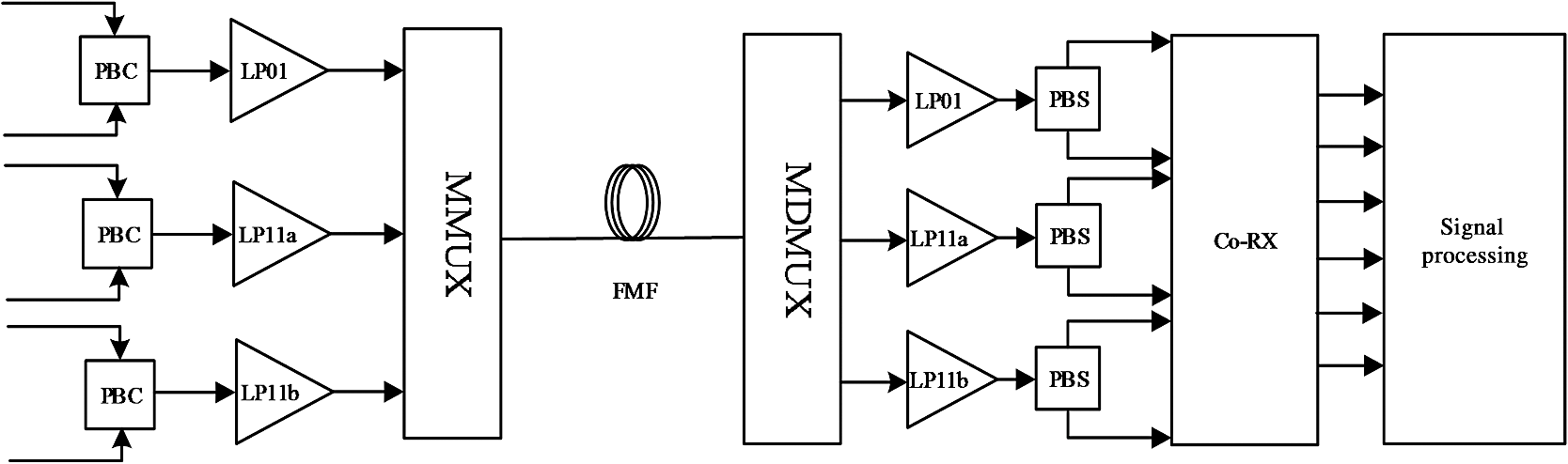
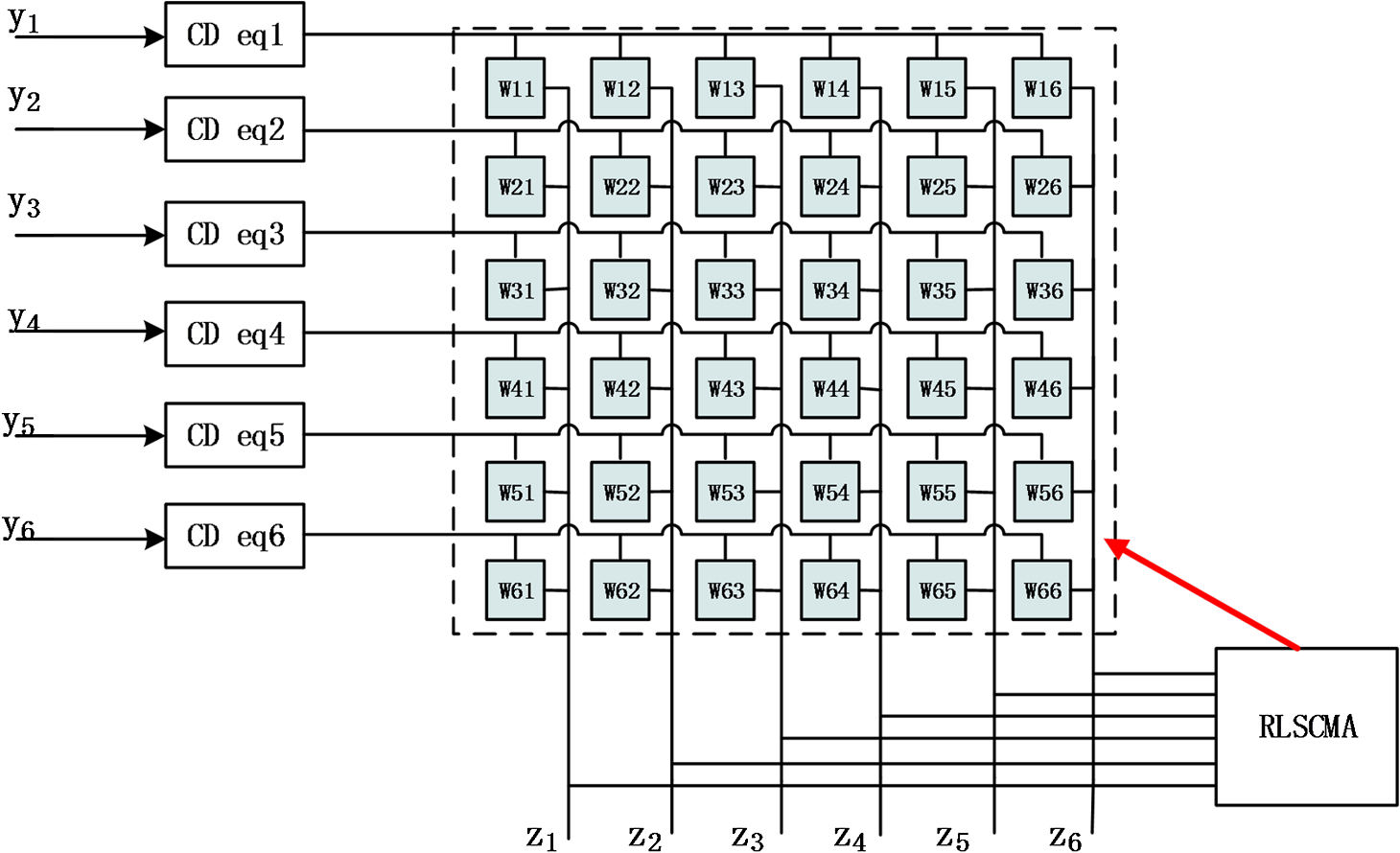
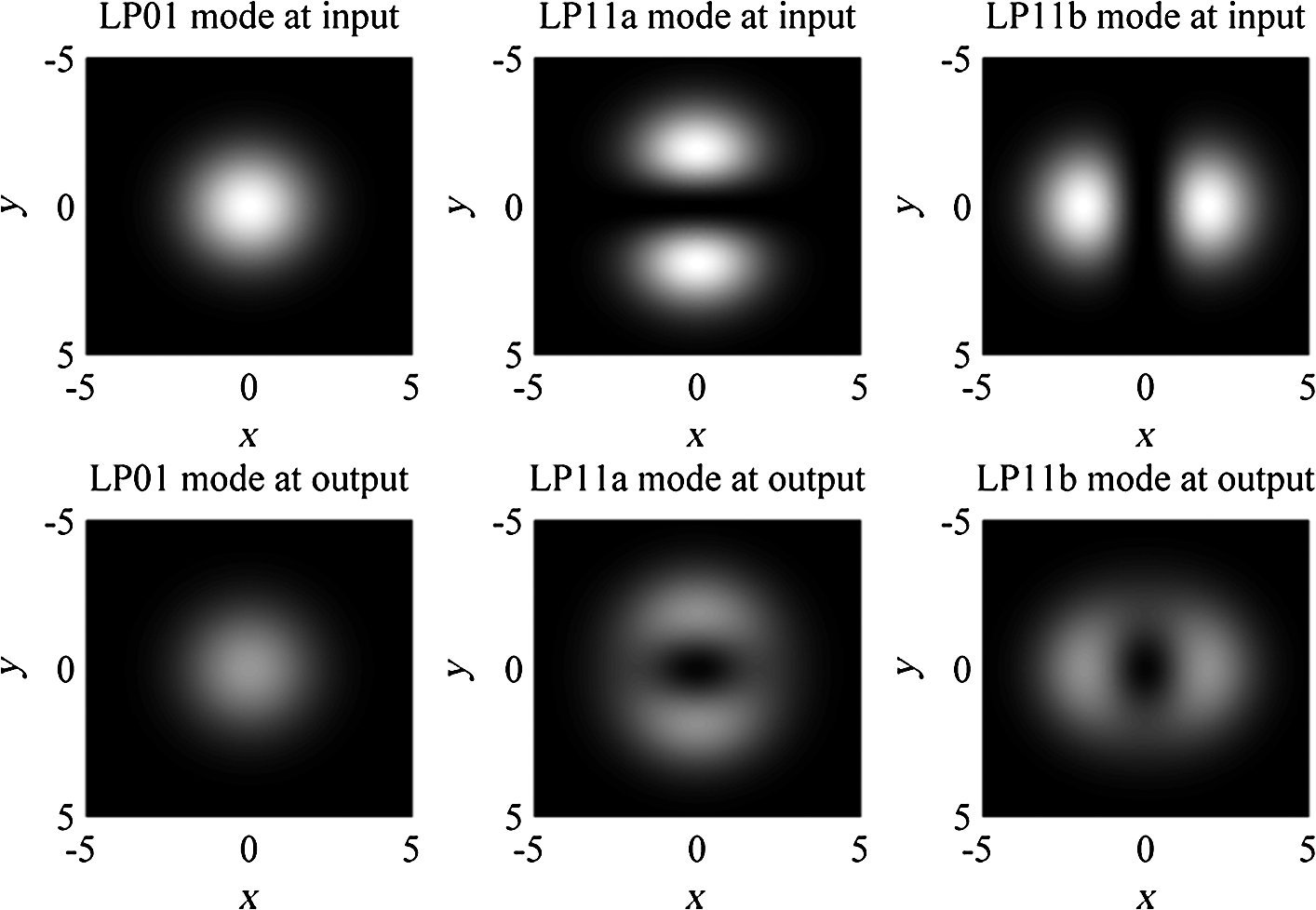
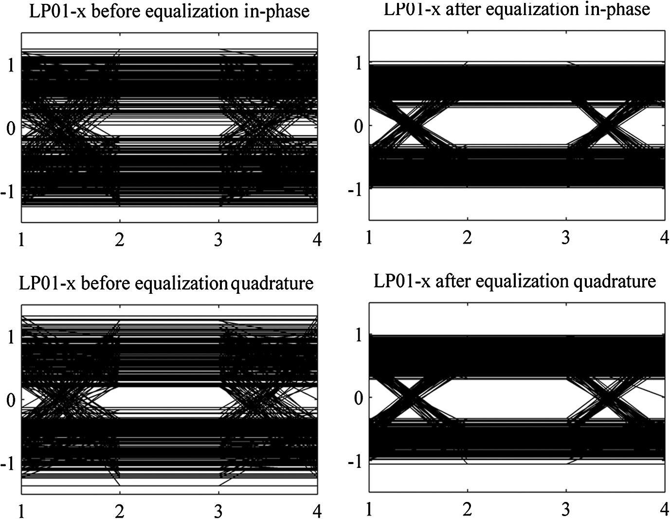
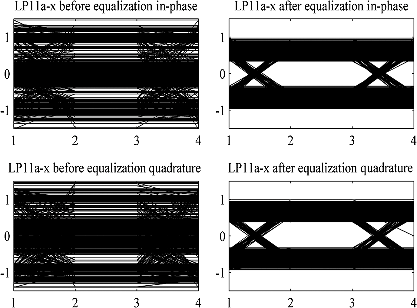
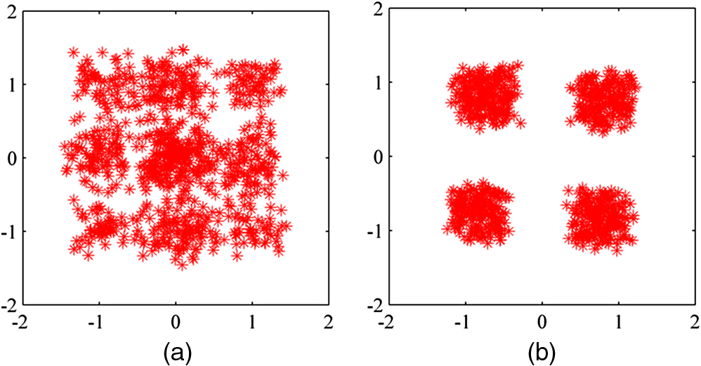
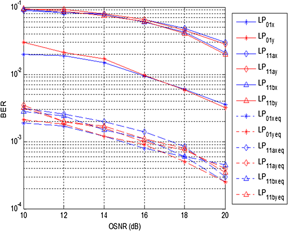
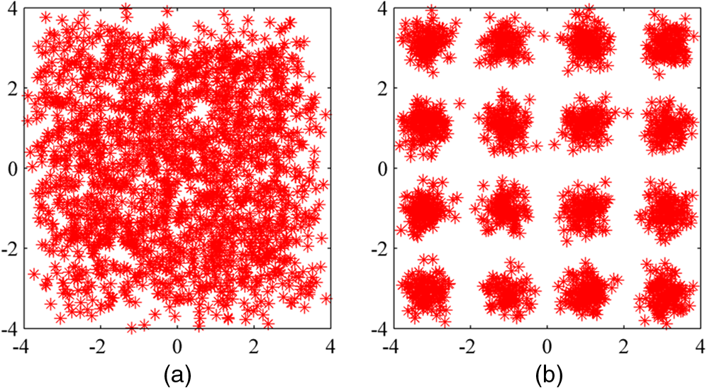
These are the basic steps of RLSCMA, and can be extended for MIMO equalization. The variable $δ$ is the norm of the input autocorrelation matrix, which is usually set as a small number when the channel status is good, and a large number with a bad channel status.

For an $N$ -mode transmission system, the matrix $P$ in the algorithm above should have a dimension of $2 N L \times 2 N L$ . For the $i$ ’th receiver, $w_{i} = [w_{i, 1}^{T}, w_{i, 2}^{T}, \dots, w_{i, 2 N}^{T}]$ are a set of $2 N$ equalizers and the equalized signal can be obtained by

Eq. (9)

z_{i} = \sum_{j = 1}^{2 N} w_{i j}^{H} \cdot y_{j},

where

w_{i}

can be obtained by the RLSCMA algorithm.

3. Simulation and Results

A $6 \times 6$ MIMO transmission system with three spatial modes (LP01 and degenerate LP11 modes) shown in Fig. 1 is simulated, where each mode carries a 20-Gbps DP-NRZ-QPSK signal. All six signals are coherently detected and sent to the signal processing unit.

Fig. 1

Block diagram of simulation.

In the simulation, the channel model consists of two parts; the channel of the multispatial mode and the channels of the polarization modes within each spatial mode are separately considered. The matrix model discussed in Sec. 2 is applied to describe the spatial mode channel, and the mode coupling matrix is approximately computed with two major vectors induced by fiber twisting, $η$ and $φ$ , where $η$ is the ratio of the random splice offset and field radius of the LP01 mode, and $φ$ is the random rotated angle between sections.⁹

The simulation parameters are set as follows: transmission length $L = 50 km$ , operating wavelength $λ_{c} = 1550 nm$ , $D = 17 ps / nm / km$ , differential mode delay between LP01 and LP11 modes $DMD = 60 ps / km$ , $φ = 0 \sim π / 8$ , $η = 0 \sim 0.1$ , $θ = π / 6$ , polarization mode delay $τ_{p} = 0.3 ps / km$ . The large effective area of FMF can suppress nonlinear effects. To simplify the analysis, nonlinear affects and mode dependent loss are ignored.

Figure 2 shows the architecture of the MIMO DSP used in this paper, where $y_{1} \sim y_{6}$ are the signals detected at the receiver, and $z_{1} \sim z_{6}$ are the outputs of the equalizer. First a group of six FIR filters is used to compensate the CD of each mode,¹⁰ then a $6 \times 6$ MIMO equalizer array consisting of 36 FIR filters operating under the RLSCMA algorithm is applied to compensate mode coupling, modal dispersion, and PMD. The number of MIMO equalizer taps is decided by the differential mode delay in the full span and symbol rate,³ where $L = ⌈ (τ_{N} - τ_{1}) r_{o s} R_{s} ⌉$ comes into 15 in this paper.

Fig. 2

Architecture of multiple-input multiple-output (MIMO) DSP.

Figure 3 shows the simulated spatial mode patterns at the input and output of the FMF, where all the orthogonal modes are affected by mode coupling. It can be seen that the degenerate LP11 modes couple with each other more severely due to spatial twists of the fiber.

Fig. 3

Mode patterns before and after transmission.

The eye diagrams of LP01-x and LP11a-x before and after equalization are compared in Figs. 4 and 5. As is depicted in the figures, the signals carried by the LP11 modes experience more severe damage than the LP01 mode, and the eye completely closes. After equalization, we achieve open eye patterns with both LP01 and LP11 modes. Because the mode pattern area of the LP01 mode is distributed in the center of the core and is larger than the LP11 modes, it suffers less influence from mode coupling induced by spatial mismatching and rotation in the applied model.

Fig. 4

Eye diagrams of LP01-x before and after MIMO equalization.

Fig. 5

Eye diagrams of LP11a-x before and after MIMO equalization.

The constellations of the signal carried by LP11a-x mode before and after MIMO equalization are shown in Fig. 6. It can be seen from the constellations that the signal received is still badly distorted due to mode coupling and mode delay after CD compensation, however, these affects can be well compensated by MIMO equalizers.

Fig. 6

Constellations of LP11a-x: (a) before and (b) after equalization.

We have also compared the RLSCMA performance with the traditional stochastic gradient descent CMA (SGDCMA). The bit error ratio (BER) curves of the two algorithms are illustrated in Fig. 7(a), where the LP11a-x mode is adopted for analysis. It can be seen that both algorithms realize an effective equalization for the received signal. Compared with SGDCMA, the required optical signal-to-noise ratio (OSNR) at BER of $10^{- 3}$ is improved by 0.5 dB with the proposed RLSCMA. Figure 7(b) shows that the RLSCMA algorithm converges more rapidly than SGDCMA (with the same equalization effect), suggesting that it is more adaptive for the complicated FMF channel.

Fig. 7

(a) Bit error ratio (BER) performance of MIMO recursive least squares constant modulus algorithm and stochastic gradient descent constant modulus algorithm and (b) mean square error convergence rates.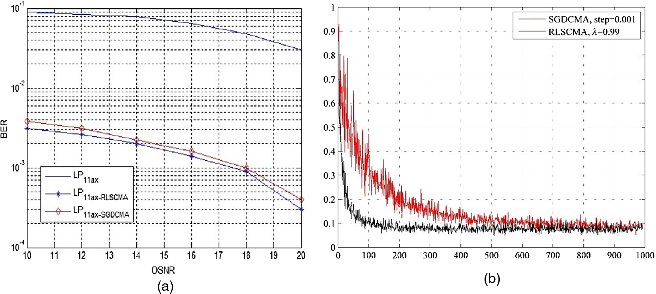

At the receiver, the signal BERs of the three modes carried on the $x$ and $y$ polarizations are calculated respectively, which are shown in Fig. 8. It can be seen that the signals on both $x$ and $y$ polarizations show similar performances after transmission. Before MIMO equalization, the received signals of the three modes suffer severe bit errors (shown by solid curves). Figure 8 also shows that the signals of the double LP11 modes have much higher BERs than that of the LP01 mode signal, which can be predicted from the eye diagrams in Figs. 4 and 5. After MIMO equalization, the BERs of all the modes are significantly decreased. The BERs below $10^{- 3}$ can be achieved for all the simulated modes with the OSNR above 18 dB. The simulation results show that MIMO RLSCMA is qualified for mode demultiplexing interference cancellation.

Fig. 8

BERs before and after equalization.

We also simulate the transmission of MDM with 16-QAM signals and do MIMO equalization with RLSCMA. The constellations before and after equalization are shown in Fig. 9, where we can see the RLSCMA performs well with 16-QAM signals.

Fig. 9

Constellations of LP11a-x 16QAM signal (a) before and (b) after equalization.

4. Conclusion

In this paper, an MIMO RLSCMA algorithm is proposed and applied to a $6 \times 6$ MDM system for signal processing. The signals on all modes are successfully recovered in the simulation, verifying that the proposed algorithm can efficiently overcome the effects of mode coupling and differential mode delay a with fast converging speed.

Acknowledgments

The financial supports from the National NSFC (No. 61425022/61275074/613070864/61475024), National High Technology 863 Program of China (No. 2013AA013403, 2015AA015501/02), NITC (No. 2012DFG12110), and Beijing Nova Program (No. Z141101001814048) are gratefully acknowledged. The project is also supported by the Universities PhD Special Research Funds (No. 20120005110003/20120005120007) and Fund of State Key Laboratory of IPOC (BUPT).

References

1.

R. Ryf et al., “Mode-division multiplexing over 96 km of few-mode fiber using coherent $6 \times 6$ MIMO processing,” J. Lightwave Technol., 30 (4), 521 –531 (2012). http://dx.doi.org/10.1109/JLT.2011.2174336 JLTEDG 0733-8724 Google Scholar

2.

E. Ip et al., “ $88 \times 3 \times 112 - Gb / s$ WDM transmission over 50-km of three-mode fiber with inline multimode fiber amplifier,” in Proc. 37th European Conf. and Exposition on Optical Communications, (2011). Google Scholar

3.

S. O. Arik, D. Askarov and J. M. Kahn, “MIMO signal processing for mode-division multiplexing: an overview of channel models and signal processing architectures,” Signal Process. Mag., 31 (2), 25 –34 (2014). http://dx.doi.org/10.1109/MSP.2013.2290804 ISPRE6 1053-5888 Google Scholar

4.

R. Roland et al., “Space-division multiplexing over 10 km of three-mode fiber using coherent $6 \times 6$ MIMO processing,” in Proc. Optical Fiber Communication Conf., (2011). Google Scholar

5.

D. R. Morgan, “An adaptive RLS MIMO equalizer algorithm for HSDPA,” in Proc. Fortieth Asilomar Conf. on Signals, Systems and Computers, 2006 (ACSSC’06), 1016 –1021 (2006). Google Scholar

6.

Y. Chen et al., “Recursive least squares constant modulus algorithm for blind adaptive array,” IEEE Trans. Signal Process., 52 (5), 1452 –1456 (2004). http://dx.doi.org/10.1109/TSP.2004.826167 ITPRED 1053-587X Google Scholar

7.

I. Fatadin, D. Ives and S. J. Savory, “Blind equalization and carrier phase recovery in a 16-QAM optical coherent system,” J. Lightwave Technol., 27 (15), 3042 –3049 (2009). http://dx.doi.org/10.1109/JLT.2009.2021961 JLTEDG 0733-8724 Google Scholar

8.

K. P. Ho and J. M. Kahn, “Mode coupling and its impact on spatially multiplexed systems,” in Optical Fiber Telecommunications VI, 491 –568 (2013). Google Scholar

9.

A. A. Juarez et al., “Perspectives of principal mode transmission in mode-division-multiplex operation,” Opt. Express, 20 (13), 13810 –13824 (2012). http://dx.doi.org/10.1364/OE.20.013810 OPEXFF 1094-4087 Google Scholar

10.

T. F. Portela et al., “Analysis of signal processing techniques for optical $112 Gb / s$ DP-QPSK receivers with experimental data,” J. Microwaves Optoelectron. Electromagn. Appl., 10 (1), 155 –164 (2011). http://dx.doi.org/10.1590/S2179-10742011000100016 Google Scholar

Biography

Xiaolong Pan is an undergraduate student at Beijing University of Posts and Telecommunications (BUPT) and a member of the State Key Laboratory of Information Photonics and Optical Communications in BUPT. His research interests focus on optical communications and optical signal processing.

Bo Liu is an assistant professor at BUPT and a member of the State Key Laboratory of Information Photonics and Optical Communications in BUPT. His research interests include broadband optical communications and optical signal processing.

Haiyuan Zhao is a student at BUPT and member of the State Key Laboratory of Information Photonics and Optical Communications in BUPT. His research interests focus on optical fiber transmission.

Qinghua Tian is an assistant professor at BUPT and a member of the State Key Laboratory of Information Photonics and Optical Communications in BUPT. She received her PhD from BUPT in 2013. Her research interests focus on optical free-space communication.

CC BY: © The Authors. Published by SPIE under a Creative Commons Attribution 4.0 Unported License. Distribution or reproduction of this work in whole or in part requires full attribution of the original publication, including its DOI.

Citation Download Citation

Xiaolong Pan, Bo Liu, Haiyuan Zhao, and Qinghua Tian "Fast convergence equalization algorithm for mode division multiplexing system," Optical Engineering 54(5), 056108 (26 May 2015). https://doi.org/10.1117/1.OE.54.5.056108

Published: 26 May 2015

Access the abstract

JOURNAL ARTICLE
6 PAGES

DOWNLOAD PAPER SAVE TO MY LIBRARY

GET CITATION

CITATIONS

Cited by 2 scholarly publications.

Explore citations on Lens.org

KEYWORDS

Optical fibers

Multiplexing

Polarization

Computer simulations

Digital signal processing

Eye

Signal detection

1.

Introduction

2.

Theory and Algorithm

2.1.

Few Mode Fiber Channel Analysis

Eq. (1)

Eq. (2)

Eq. (3)

Eq. (4)

Eq. (5)

Eq. (6)

2.2.

Recursive Least Squares Constant Modulus Algorithm

Eq. (7)

Eq. (8)

Eq. (9)

3.

Simulation and Results

Fig. 1

Fig. 2

Fig. 3

Fig. 4

Fig. 5

Fig. 6

Fig. 7

Fig. 8

Fig. 9

4.

Conclusion

Acknowledgments

References

Biography

Show All Keywords

Keywords/Phrases

Search In:

Publication Years