1.

Introduction

Light beams having optical vortices (OVs) or phase singularities^1–4 have been attracting much interest because of their wide range of applications, such as information encoding,⁵ optical manipulation,^6,7 stimulated emission depletion microscopy,⁸ optical metrology,^9,10 and so on. The phase structure of an OV has a helical waveform that varies continuously from 0 to $2n\pi$ rad (where $n$ is an integer called the topological charge), and the center of the phase structure is a singular point with zero amplitude and an undefined phase. OV beams can be produced by components such as spiral phase plates and holograms. By using a spatial light modulator (SLM) to display suitable holographic patterns, various high-quality OV beams can be easily realized.¹¹ To meet increasing demands for improved performance, adaptive real-time control of the OV beams is needed,^4,12 which requires simple and reliable measurement techniques.

Several methods have been proposed for determining the positions of singular points in an OV beam. Interferometry is a well-known method and gives good measurement accuracy and high-spatial resolution.^13,14 Interferographic measurement is, however, very sensitive to the environmental conditions, such as vibrations and temperature variations. Also, relatively complicated optics is required. Recently, a Shack–Hartmann wavefront sensor (SH-WFS) has been used to overcome these problems.¹⁵ The SH-WFS simply consists of a lenslet array and an image sensor and measures the phase slope vectors of an incoming wavefront. Therefore, a distribution of phase slope vectors can be easily obtained.

The basis of OV detection using the SH-WFS is that the contour sum of the phase slope vectors along a closed path is nonzero if there is a net topological charge of the phase singularities enclosed by the closed path.^2,16 The presence and absence of phase singularities in a light beam can be determined according to the nonzero (local peak) values of the contour summations. Some improvements and modifications have been made to reduce noise;^17–19 however, the spatial resolution of measurements with the SH-WFS is limited by the lens size of the lenslet array.

To detect singular points in an OV beam with sublens-size spatial resolution, we have proposed a correlation matching method (CMM).^20,21 The CMM can be applied to detect more than one singular point, and an example in which a pair of singular points in a beam is detected is given in Ref. 21. This method involves calculating circulations that are the discrete contour integrals of phase slope vectors along a closed path connecting the centers of $2\times 2$-neighboring lenslet apertures and comparing the circulations with a set of precalculated reference values. The estimated precision was better than 0.1 in units of the lens size. However, we found that the measurement errors depend on the positional relationship between the singular point being detected and the closed path applied as a result of the low-intensity region existing around the singular points in the OV beam. We have, therefore, proposed a hybrid centroiding method (HCM) to reduce the distribution error resulting from this positional relationship.²² In the HCM, the window size for the centroid calculation varies according to the magnitude of the circulations. To reduce the influence of the low-intensity regions existing around the singular points, we have also proposed a phase-slope-combining CMM.²³ By using this method, the position-detection precision could be maintained at better than 0.15 (lens-size) even when detecting an OV beam with a topological charge of up to 20. In all of these SH-WFS–based methods, the circulation values related to the phase slope distribution are calculated using the closed paths connecting the centers of $2\times 2$-neighboring lenslet apertures.

In this paper, we propose an alternative approach to realize detection of singular points in an OV beam with sublens-size spatial resolution. An extended closed path that encloses a larger area than the conventional $2\times 2$-closed path is applied to calculate circulations. Because a phase singularity may be surrounded by a low-intensity region that increases the inaccurate phase slopes being measured, using a large closed path could reduce the influence of the low-intensity region, thus higher detection accuracy could be expected. Also, the circulation calculated using a large contour is closer to that obtained from the theoretical continuous integral. This would be beneficial for charge detection. However, the ability to distinguish multiple vortices becomes lower when using larger contours. Therefore, in this study we use a closed path associated with $3\times 3$-neighboring lenslet apertures and demonstrate its usefulness for accurately detecting the positions of phase singularities.

Also, to achieve accurate measurement and a shorter computing time, we use a simple centroiding calculation with a fixed window size instead of either the time-consuming correlation-matching computation²⁰ or the relatively complicated hybrid centroiding framework. ²² The remainder of the paper is organized as follows. In Sec. 2, we describe our method. In Sec. 3, we present an optical setup for performing proof-of-principle experiments, and in Sec. 4, we present experimental results and discussions. A summary and conclusions are provided in Sec. 5.

2.

Method

2.1.

Eight-Connected Closed Contour for Optical Vortex Detection

An optical vortex beam is an optical field that has phase singularities. Generally, the presence of phase singularities in a phase function can be determined with the aid of a closed-line integral over the gradient of the phase function:¹⁶

Eq. (1)

$${\oint }_C\nabla \varphi ·\mathrm{d}\overrightarrow{l}=2n\pi ,$$

where $C$ is the closed path of the integration contour, $\nabla \varphi$ is the gradient of a phase function $\varphi (x,y)$, $\mathrm{d}\overrightarrow{l}$ is the infinitesimal element of the contour, and integer $n$ represents the net topological charge of all the phase singularities enclosed by the contour $C$. Equation (1) indicates that the result of the contour integration is nonzero if $n\ne 0$, or zero if $n=0$.

In practice, to detect phase singularities using a device, we must define the closed path according to the structure of the device, and accordingly rewrite Eq. (1) with measurable parameters. Previous studies used a closed path associated with $2\times 2$-neighboring measurement points.^16–22 Instead, here we propose an alternate closed path that connects the centers of the eight nearest neighbors of measurement points, which we call an eight-connected contour in the rest of this paper (Fig. 1).

Fig. 1

Concept of circulation calculation with closed path passing through the centers of eight connected lenslet apertures. ($s_x^{i,j},s_y^{i,j}$) represents the phase slope vector measured at the ($i^{\prime },j^{\prime }$)-th lenslet. The red dashed line indicates a closed path for the circulation calculation. Solid circles represent the centers of lenslet apertures, and the open circle is the point where the circulation is assigned, which is also the center of the closed path. The circled plus sign denotes the position of the singular point.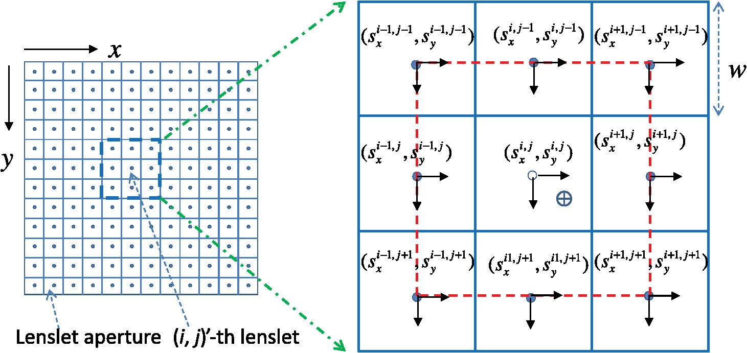

We consider that an SH-WFS consists of a square-grid lenslet array and an image sensor. A discrete version of the contour integration of the left side of Eq. (1) can be written as

Eq. (2)

$$D(i,j)=w\times \sum _{k=-1}^1{\epsilon }_k(s_x^{i+k,j-1}-s_x^{i+k,j+1}+s_y^{i+1,j+k}-s_y^{i-1,j+k}),{\epsilon }_k=\{\begin{array}{ll}1& k=0\\ 0.5& k\ne 0\end{array},$$

where $w$ is the size of the lenslet aperture and ($s_x^{i,j},s_y^{i,j}$) is the phase slope vector measured at the ($i^{\prime },j^{\prime }$)-th lenslet point. $D(i,j)$ can be considered as a value that is related to the phase slope vector distribution and is called the circulation at point ($i,j$) that is the central point of the ($i^{\prime },j^{\prime }$)-th lenslet aperture.

Figure 1 shows a conceptual diagram of this circulation calculation. In Fig. 1, the $x$-axis is from the left to the right, and the $y$-axis is from the top to the bottom. The closed path for the circulation calculation denoted by the red dashed line passes through the centers of the eight-connected neighboring lenslet apertures. In Fig. 1, ($s_x^{i,j},s_y^{i,j}$) represents the phase slope vector measured at the ($i^{\prime },j^{\prime }$)-th lenslet point. Solid circles represent the centers of the lenslet apertures, and the open circle is the central point of the closed path, at which point the circulation is assigned. The circled plus sign denotes the position of the singular point.

It should be mentioned that the ($i^{\prime },j^{\prime }$)-th circulation $D(i,j)$ defined by Eq. (2) does not include the phase slope vector data at the ($i^{\prime },j^{\prime }$)-th lenslet point, but only depends on its eight-connected neighborhood. Suppose that a phase singularity exists within the aperture of the ($i_0^{\prime },j_0^{\prime }$)-th lenslet, and no phase singularity exists in its surrounding lenslet apertures ($i_0+k,j_0+l$) ($k,l=1,-1$). Then the low-intensity region of the OV beam may influence the measurement of the ($i^{\prime },j^{\prime }$)-th phase slope vector but will have no or less influence on the measurements of its eight neighbors. Therefore, higher detection accuracy is expected in comparison with that using a conventional $2\times 2$ contour.

Although $D(i,j)$ is a discrete approximation of the closed-line integral, it has a special distinguishing characteristic. Studies have shown that the circulation approaches zero (ignoring noise) in the case where no singularity exits in the contour region; however; if there is net topological charge within the ($i_0^{\prime },j_0^{\prime }$)-th lenslet aperture, then the circulation $D(i_0,j_0)$ approaches its local maximum, and its eight neighbors $D(i_0+k,j_0+l)$ $(k=\pm 1,l=\pm 1)$ tend to have nonzero values. Furthermore, the circulations of the eight neighbors depend on the location of the singular point: If the singular point is at the center of the ($i_0^{\prime },j_0^{\prime }$)-th lenslet aperture, the circulation $D(i_0,j_0)$ is a local maximum, and its eight neighboring circulations are approximately half of the local maximum. In contrast, when the OV is displaced away from the center, the circulation $D(i_0,j_0)$ is almost constant, but its eight neighbors tend to vary linearly with the distance from the center. This characteristic is quite different from that using a $2\times 2$ contour.¹⁶

From the above analysis, the displacement (${\mathrm{\Delta }}_x,{\mathrm{\Delta }}_y$) from the local peak position can be obtained by

Eq. (3)

$${\mathrm{\Delta }}_x=\frac{\sum _{k=-1}^{k=1}\sum _{l=-1}^{l=1}kD(i_{\max }+k,j_{\max }+l)}{\sum _{k=-1}^{k=1}\sum _{l=-1}^{l=1}D(i_{\max }+k,j_{\max }+l)},$$

Eq. (4)

$${\mathrm{\Delta }}_y=\frac{\sum _{k=-1}^{k=1}\sum _{l=-1}^{l=1}lD(i_{\max }+k,j_{\max }+l)}{\sum _{k=-1}^{k=1}\sum _{l=-1}^{l=1}D(i_{\max }+k,j_{\max }+l)},$$

and

Eq. (5)

$$(i_{\max },j_{\max })=\max \mathrm{pos}[|D(i,j)|],$$

where $(i_{\text{max}},j_{\text{max}})$ is the peak position, and maxpos() is an operation of searching for the local maximum and returning the position where the local maximum is found. Consequently, the position $(u_{\mathrm{ov}},v_{\mathrm{ov}})$, in units of lens size, of the singular point is determined by combining the position of the local peak and the displacement from the peak position:

Eq. (6)

$$\begin{gathered} u_{\mathrm{ov}}=i_{\max }+{\mathrm{\Delta }}_x \\ {v}_{\mathrm{ov}}=j_{\max }+{\mathrm{\Delta }}_y. \end{gathered}$$

2.2.

Numerical Analysis of Measurement Accuracy

To confirm the measurement accuracy of the proposed eight-connected contour method, we performed simple numerical calculations. In the simulation, an OV beam whose singular point position was set in advance was made incident on the SH-WFS. The circulations obtained with the conventional $2\times 2$ contour and our proposed eight-connected contour were calculated individually. A nine-point centroid method, involving the $3\times 3$-elemental circulations around the peak circulation, was used to determine the position of the singular point in each case. At each location, the errors between the true position and the centroiding position were calculated using

Eq. (7)

$$E(u_0,v_0)=\sqrt{{(u_{\mathrm{ov}}^{u_0,v_0}-u_0)}^2+{(v_{\mathrm{ov}}^{u_0,v_0}-v_0)}^2},$$

where $u_{\mathrm{ov}}^{u_0,v_0}$ and $v_{\mathrm{ov}}^{u_0,v_0}$ indicate the OV’s positions calculated by the centroid method in the horizontal and vertical directions, and ($u_0,v_0$) is the position of the preset singular point. Figures 2 and 3 show the error distribution $E(u_0,v_0)$ for the eight-connected and $2\times 2$ contours, respectively. The error distributions represented as a one-dimensional function of $r=\sqrt{u^2+v^2}$ are shown in Figs. 2(b) and 3(b) for $v=0$ (middle line), $v=0.5$ (edge line), and $v=u$ (diagonal line).

Fig. 2

(a) Calculated two-dimensional (2-D) error distribution and (b) one-dimensional (1-D) profiles along $v=0$ (middle line), $v=0.5$ (edge line), and $v=u$ (diagonal line) for eight-connected contour. The coordinate (0, 0) is the central point of the lenslet aperture.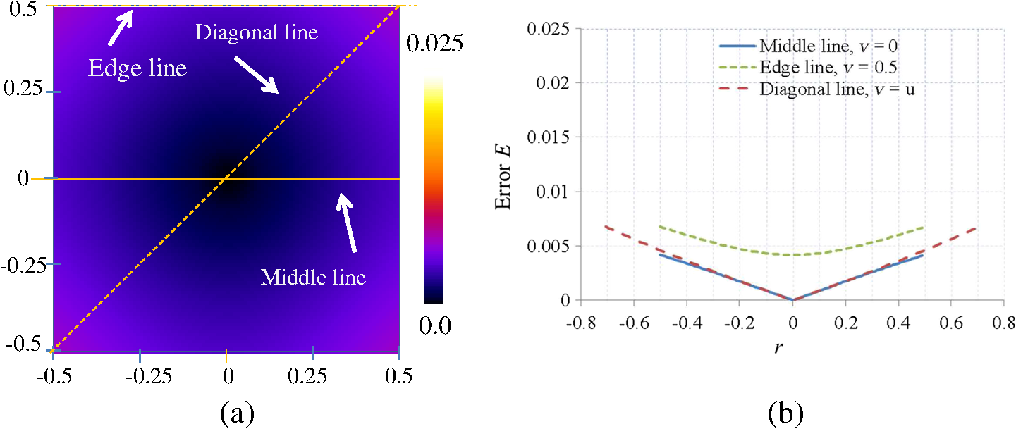

Fig. 3

(a) Calculated 2-D error distribution and (b) 1-D profiles along $v=0$ (middle line), $v=0.5$ (edge line), and $v=u$ (diagonal line) for $2\times 2$ contour. The coordinate (0, 0) is the cross-point of the $2\times 2$ lenslet apertures.

Both error distributions showed similar symmetrical characteristics, but the eight-connected contour method performed better than the $2\times 2$ contour method. In the case of the eight-connected contour, the geometrical center of the contour is consistent with the center of the central lenslet aperture. The error is zero when the phase singularity is located exactly at the center of the central lenslet aperture. The error tends to become larger the farther the phase singularity is located from the center. The error tends to be largest when the phase singularity is located in the corner of the central lenslet aperture, that is, at the cross-point of the $2\times 2$-lenslet apertures. The maximum error was smaller than 0.008 (lens-size). On the other hand, in the case of the $2\times 2$ contour, the center is consistent with the cross-point of the $2\times 2$-lenslet apertures, where the error is zero. The error tends to become larger the farther the phase singularity is located from the cross-point. The maximum error was larger than 0.022 (lens-size), which is approximately three-times larger than that of the eight-connected case. The result shows that the eight-connected contour performed better than the $2\times 2$ contour.

3.

Experimental Setup

A schematic diagram of the setup used for performing proof-of-principle experiments is depicted in Fig. 4.²⁰ A collimated beam from a HeNe laser (wavelength 633 nm), with almost uniform intensity distribution, passed through an aperture (6 mm in diameter) and illuminated a liquid-crystal-on-silicon SLM (LCOS-SLM), on which spiral phase patterns (SPPs) were displayed. The beam was transformed into an OV beam after being reflecting back from the LCOS-SLM. The beam was then split in two by a beam splitter (BS2). One beam passed through a $4\text{-}f$ system composed of two lenses (Lens 1 with $f=250\mathrm{mm}$ and Lens 2 with $f=400\mathrm{mm}$), and arrived at the SH-WFS and an image sensor (CMOS 1). Both SH-WFS and CMOS 1 were set at the conjugate planes of the LCOS-SLM. The other beam split by the BS2 went to a second image sensor (CMOS 2) located at the focal plane of a third lens (Lens 3 with $f=250\mathrm{mm}$) to check the quality of the OV beam. We also added a blazed-grating-type phase pattern onto the spiral phase pattern and used a spatial filter (3 mm in diameter) at the focal plane of Lens 1 so that only the first-order light arrived at the wavefront sensor and CMOS 1.

Fig. 4

Schematic diagram of the experimental setup. SH-WFS, Shack-Hartmann wavefront sensor; LCOS-SLM, liquid-crystal-on-silicon spatial light modulator; BS1, BS2, BS3, beam splitters; CMOS 1, CMOS 2, and CMOS image sensors.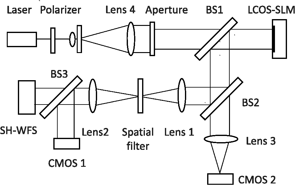

The LCOS-SLM used in our experiment was a phase-only modulation device (Hamamatsu Photonics, X10468-01), with $792\times 600$ pixels, and each pixel had dimensions of $20\mu \mathrm{m}\times 20\mu \mathrm{m}$.²⁴ The SH-WFS consisted of two elements: a lenslet array of $200\text{-}\mu \mathrm{m}$ pitch and 11-mm focal length, and a high-speed intelligent vision sensor (Hamamatsu Photonics, C8201) with $512\times 512$ pixels and a pixel size of $20\mu \mathrm{m}\times 20\mu \mathrm{m}$.²⁵

4.

Results and Discussion

In the experiments, we generated various OV beams of different topological charges by displaying suitable SPPs on the LCOS-SLM and acquired Hartmanngrams with the SH-WFS. The positions of singular points in the OV beams were calculated from the Hartmanngrams.

To test the basic performance of the experimental setup, we first observed intensity images of the generated OV beams. Figure 5 shows an example of the spiral phase pattern displayed on the LCOS-SLM (a), the conjugate intensity distribution captured by CMOS 1 (b), and the far field image captured by CMOS 2(c). In Fig. 5(a), the spiral phase pattern was larger than 6 mm in diameter. The phase values were wrapped into the interval from 0 to $2\pi$ rad and are represented by gray-scale brightnesses. In Fig. 5(b), we can see a clear low-intensity region in the conjugate image. The diameter of the low-intensity region was found to depend on both the topological charge and the diameter of the spatial filter used in the experiments. We believe the low-intensity region is due to the spiral phase structure of the OV beam and its propagation through the optical system. In the far-field image in Fig. 5(c), a donut-shaped intensity distribution having a constant-intensity circular contour is clearly visible.

Fig. 5

(a) Spiral phase pattern displayed on the LCOS-SLM for generating an optical vortex beam of topological charge $n=1$; (b) intensity image obtained at the conjugate plane of the LCOS-SLM captured by CMOS 1; and (c) far-field image obtained at the focal plane of Lens 3 captured by CMOS 2. The scale bar is 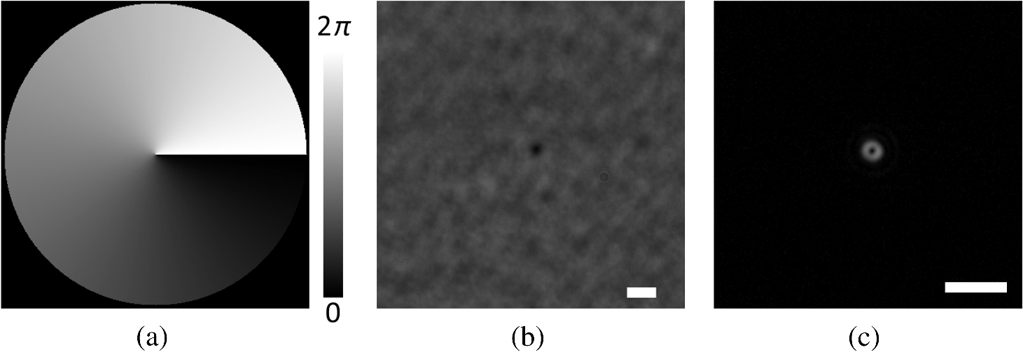$200\mu \mathrm{m}$.

Figure 6 shows an example of the measurement, showing (a) a Hartmanngram, (b) a circulation distribution calculated from the Hartmanngram, and (c) several circulation values around the peak position. The peak was found at (26, 25) and is marked by the red dashed square in Fig. 6(c), and the displacement calculated by the nine-point centroid method, that is, the $3\times 3$ elements around the peak, was (0.18, 0.62). Thus, the measured position of the singular point in the OV beam was (26.18, 25.62), in units of lens size.

Fig. 6

(a) Example of Hartmanngram, (b) circulation distribution, and (c) actual values of circulation around the peak position. The local peak is marked by the red dashed square.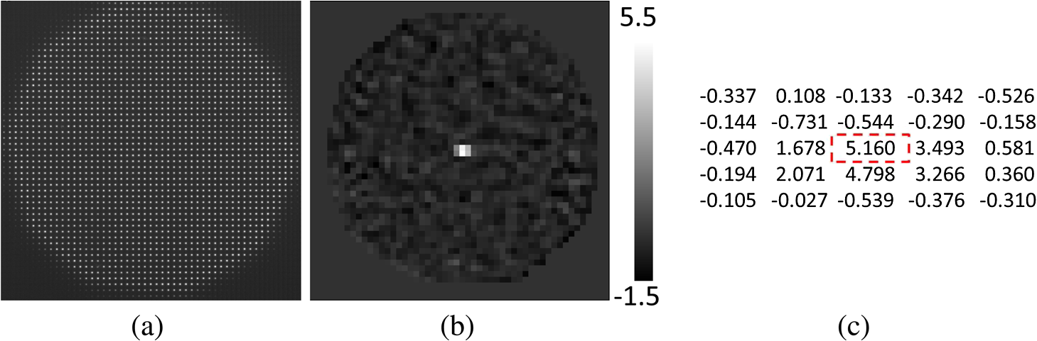

Figure 7 shows the result of detecting two vortices having topological charges 1 and $-1$. In Fig. 7, (a) shows the phase pattern where two singular points were designed to have a spacing of about 3 lens-sizes in both the x- and y-directions, (b) is the Hartmanngram, and (c) is the circulation distribution. Peaks with positive and negative circulations were found in Fig. 7(c). The measured positions of the two vortices were (16.08, 15.86) and (19.15, 18.88), respectively. Accordingly the spacings were 3.07 (lens-size) in the $x$-direction and 3.02 (lens-size) in the $y$-direction.

Fig. 7

(a) Phase pattern for generating a pair of phase singularities of topological charges 1 and $-1$, (b) Hartmanngram, and (c) circulation distribution.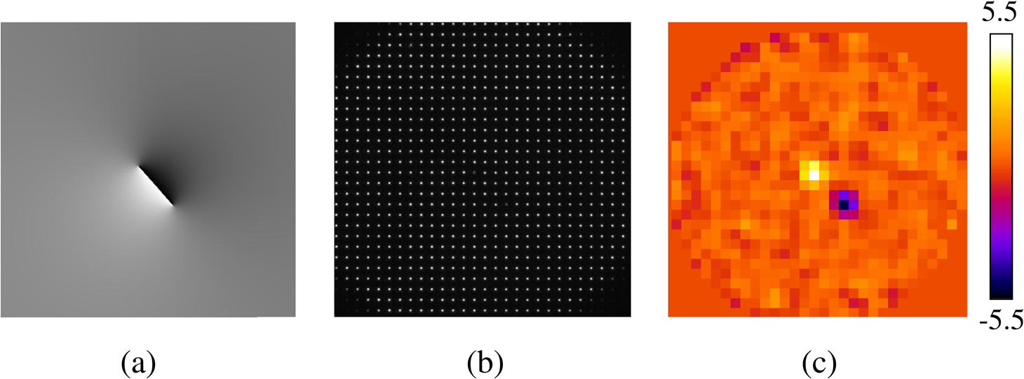

The accuracy of the measurement was confirmed experimentally. We generated various OV beams of different topological charges and shifted them two-dimensionally to different locations by displacing the spiral phase pattern on the LCOS-SLM. Figure 8 shows the graphs of the measured positions of the singular point as functions of the horizontal displacements of the SPPs on the LCOS-SLM for topological charges $n=\mathrm{1,2},3$, and 4. The left and right graphs in Fig. 8 are the $x$- and $y$-components of the measured positions, respectively.

Fig. 8

Plots of measured positions versus the displacement of the spiral phase pattern on the LCOS-SLM for topological charges $n=\mathrm{1,}2,3$, and 4, and theoretical predictions, for (a) the horizontal component and (b) the vertical component.

In Fig. 8(a), we could obtain good linearity between the measured horizontal component and the horizontal displacement applied. The slopes of the linear fitting lines are 0.160, 0.156, 0.158, and 0.155 for the topological charges $n=\mathrm{1,2},3$, and 4, respectively. According to our optical setup, a one-pixel displacement ($=20\mu \mathrm{m}$) on the LCOS-SLM plane corresponded to a $31.6\text{-}\mu \mathrm{m}$ displacement on the SH-WFS plane, or 0.158 in units of lens size. Therefore, the slope results agreed well with the theoretical predictions [the dashed line in Fig. 8(a)]. The measured vertical components for the horizontal displacements were almost constant, as shown in Fig. 8(b). Statistical analysis showed that the root-mean-square error (RMS) over the measurements of the $15\times 4$ positions and the four charges was approximately 0.09 (lens-size), which is comparable to that obtained with the CMM^20,21 and HCM.²²

Figure 9 shows comparisons of the measured results obtained by the proposed eight-connected contour method (blue filled diamonds) and the conventional $2\times 2$ contour method (red open squares). In Fig. 9, the $y$-axis shows the difference between the measured position and the theoretical prediction. As shown in Fig. 9, the result obtained with the proposed eight-connected contour method had a smaller error than that obtained with the $2\times 2$ contour method. The maximum of the absolute difference between the measured position and the theoretical prediction was less than 0.1 (lens-size) for the eight-connected contour method, and 0.24 (lens-size) for the $2\times 2$ contour method, respectively. Figure 9 also shows the results obtained with the CMM, which are represented by the red open circles.

Fig. 9

Comparison of singular point positions measured by the proposed eight-connected contour centroid method (blue filled diamonds), the conventional $2\times 2$ contour centroid method (red open squares), and the correction matching method (red open circles).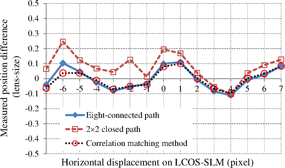

We also estimated the topological charges of the phase singularities being detected. Figure 10 shows the measured topological charges of the phase singularities versus the topological charges of the SPPs for generating the phase singularities. The open bars are the charges with an eight-connected path, and the hashed bars are those with a $2\times 2$ closed path. The topological charges were measured simply as the ratio of the local maximum circulation to a closed-path-associated coefficient. The coefficient was about 5.22 for the eight-connected path and 3.14 for the $2\times 2$ closed path, which were determined by experiments conducted in advance. In Fig. 10, the measured topological charges are the averaged ones over the measurements corresponding to the 15 horizontal displacements of the SPPs shown in Fig. 8. The obtained topological charges are noninteger numbers, but are very close to the integer values of the topological charges applied. In Fig. 10, the error bars represent the deviations of the measured topological charges from the integer values of the topological charges applied, which are given by

Fig. 10

Measured topological charges of phase singular points versus the topological charges of the spiral phase patterns for generating the phase singularities.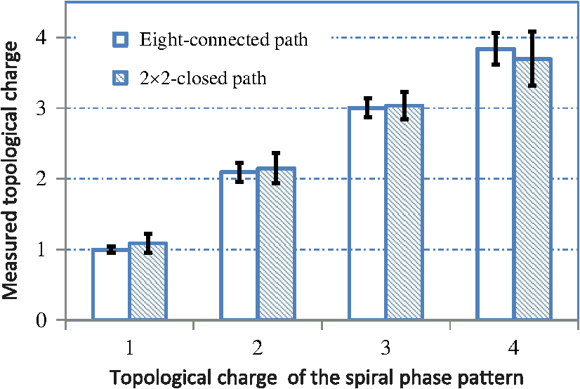

The experimental results showed that the measurement accuracy of the proposed eight-connected contour method was comparable to that of the CMM. The new method uses a simple centroid calculation, thus the computing time can be dramatically reduced in comparison with CMM.²⁰ It does not need the relatively complicated hybrid centroid framework.²² The method simplifies the calculation procedure while maintaining its high position-detection accuracy, and can be applied to real-time control applications.

A major factor that affects the detection accuracy is the low-intensity regions around the singular points in the OV beam. As shown in Fig. 5(b), a low-intensity region could be observed even though it was taken at the conjugate plane of the LCOS-SLM where the collimated beam is converted into an OV beam. Generally, the low-intensity regions will be wider and have rather softer edges when the light propagates through free space. Within this region, the Hartmanngram spots may be deformed, and in the worst case, one or more spots may disappear, as shown in Fig. 5(a). However, this problem could be solved by using a phase slope combination technique.²³

Another practical issue related to singular point detection is the cases of light beams that have more than one phase singularity. The proposed method is able to detect multiple-phase singularities, but there are some limitations. A major limitation is that it is impossible to distinguish individual phase singularities that are enclosed by the same closed path by using the contour methods. The minimum spacing of two phase singularities that can be independently located is two lens-sizes in the case of using the eight-connected closed path, which is two times larger than that using the $2\times 2$ closed path. Reducing the spacing to less than the minimal spacing tends to greatly increase the detection error, and detection finally becomes impossible.

5.

Conclusion

In conclusion, we have proposed a new simple SH-WFS-based method for detecting singular points in an OV beam with sublens-size spatial resolution. The method first calculates circulations using the phase-slope vector data measured by the SH-WFS, and then determines the accurate positions of singular points via a centroid calculation. We used an eight-connected, instead of a $2\times 2$ contour in the circulation calculation. Both a numerical analysis and a proof-of-principle experiment showed that the proposed eight-connected contour method has a better performance than the conventional $2\times 2$ contour method. In the experiments, we used an LCOS-SLM for generating various OV beams by displaying various SPPs on it. The positions of singular points in the OV beams were measured at the conjugate plane of the LCOS-SLM. We obtained good linearity between the measured shifts of the singular point and the displacements of the SPPs on the LCOS-SLM. The RMS error of the measured positions of the singular points was about 0.09 (lens-size). In comparison with the previously used CMM and HCM methods, the new method stands out by its reduced implementation time and improved signal-to-noise ratio, and is, therefore, more suitable for real-time control applications.

To develop a simple and reliable technique for measuring an optical vortex beam, in this study, we tested our new method in a well-controlled situation; that is, phase singularities are generated on an SLM, and the conjugated image is detected by an SH-WFS. Many applications, such as optical manipulation, use the far-field images. Also, in most real-time control applications, the propagation steps of an OV beam, which will cause a more-complex optical field, should be considered. Therefore, further research along this direction is necessary so that the SH-WFS can be applied to these realistic situations.