
|
|
1.IntroductionThe threat quantum computing poses to public key cryptography is motivating the development of alternatives to modern key sharing techniques that rely on computational complexity for security.1,2 Presently, there is interest in developing quantum key distribution (QKD), presented by Bennett and Brassard in 1984 (BB84), as a provably secure alternative.2–5 QKD lends itself to mathematical proofs of theoretical security and offers the potential for secure generation of symmetric encryption keys in real time over optical channels.6,7 The BB84 QKD protocol generates encryption keys using polarization states of light transmitted and detected via individual photons. Attempts by an eavesdropper to intercept, clone, and resend individual photons lead to errors in the cloned states that in turn lead to bit errors, referred to as quantum bit errors.3,8 Quantum bit errors can be detected by the key sharing parties to reveal the presence of the eavesdropper. Based on the assumption that a technologically advanced eavesdropper could suppress naturally occurring bit errors, all bit errors are assumed to be due to eavesdropping and an indication of information leakage. This includes bit errors that may in actuality be due to scattered light, detector dark counts, and channel crosstalk. The inferred information leakage is mitigated with privacy amplification algorithms that reduce the number of key bits.9 For sufficiently large quantum bit error rates (QBERs), secure key generation (SKG) is not possible.10 It is therefore important to consider technologies that minimize naturally occurring sources of bit errors. Concepts for global QKD networks include the use of free-space quantum channels linking ground- and space-based nodes.11–13 Demonstrations of free-space QKD have been carried out successfully, including implementations over terrestrial12,14–18 and ground-air quantum channels.18,19 Free-space quantum channels present a number of practical challenges for QKD. The scattering of ambient light into the quantum channel can be a significant source of quantum bit errors. Signal transmission efficiencies are reduced by beam divergence, atmospheric scattering and absorption, and atmospheric-turbulence-induced wavefront errors. The mechanisms of noise and loss both contribute to increased QBERs that can preclude SKG. Terrestrial demonstrations of free-space QKD in daylight have utilized spectral and temporal filtering techniques to reduce noise due to scattered light. This includes a demonstration conducted at a low daytime sky radiance using a dielectric spectral filter14 and a demonstration conducted at significantly higher radiance using an atomic-line spectral filter.15 System-level analyses for implementations linking low-Earth orbit (LEO) satellites to terrestrial ground stations support plans for full-scale satellite demonstrations.18,20–27 Studies have considered both upward and downward propagating signal photons and concluded downlinks offer the advantage of lower transmitter-to-receiver aperture coupling losses due to the effects of atmospheric turbulence.13,22 In the downlink scenario, the receiver points toward the sky. In this scenario, sky radiance can be a significant source of quantum bit errors in daytime. Analyses of daytime satellite QKD downlinks have assumed a variety of sky radiance values under cloud-free conditions.20,22,28 Recently, we presented an analysis of hemispherical distributions of daytime sky radiance and QBERs associated with satellite transmitters in circular orbits under clear sky conditions.29 Spatial filtering can also mitigate sky noise in a QKD downlink receiver. This is accomplished by reducing the receiver field of view (FOV). Atmospheric turbulence limits the extent to which this can be done without introducing signal loss. FOVs previously discussed in the literature are sufficiently large to avoid turbulence-induced signal loss.14–16,18,22,24 It has been discussed that improved tracking, or wavefront tilt correction, in a QKD receiver can improve the signal at small FOVs.17,20,30,31 Recently, we presented preliminary results from numerical simulations showing that implementing higher-order adaptive optics (AO) at reduced FOVs in a QKD ground-station receiver can significantly improve SKG rates in daytime and enable SKG under conditions where it would otherwise be prohibited.32 The concept of real-time sensing and correction of atmospheric-turbulence-induced wavefront errors was proposed in 1953 by Babcock.33 The first practical design for atmospheric compensation was proposed, patented, and demonstrated in the mid-1970s by Hardy while working for Itek optical systems.34–36 Compensated imaging of LEO satellites was first accomplished in 1982 by the Air Force under funding from the Advanced Research Projects Agency.36 This demonstration was followed by the rapid development of supporting and enabling technologies.36–38 In modern AO systems, low-order and higher-order wavefront errors are treated separately. Low-order errors corresponding to linear wavefront tilts are compensated with steering mirrors. Higher-order errors are compensated using two-dimensional wavefront compensating optics. Optimized compensation of dynamic wavefront errors requires closed-loop control of the AO system at a bandwidth that typically exceeds the rate at which turbulence is changing.39 Where telescope slewing is involved, the wavefront error includes a translational component associated with both wind and slewing. This translational component is described by the Greenwood frequency.39 High Greenwood frequencies associated with tracking a LEO satellite through turbulence can challenge the performance capabilities of an AO system. Atmospheric turbulence is a stochastic process. Consequently, propagation through turbulence leads to statistical distributions of wavefront errors. In a free-space quantum channel, this can lead to statistical distributions of SKG rates. Quantifying the effects of turbulence and AO on SKG rates requires numerical simulations. The Air Force Research Laboratory sponsored the development of fully integrated software that accurately models both the effects of wave propagation through the atmosphere and AO compensation.40,41 The software propagates optical wavefronts through statistical representations of turbulence and through the optical components of an AO system including the time-dependent behavior of these components under closed-loop control. This paper considers a LEO satellite QKD downlink to a terrestrial receiver that includes an AO system. Numerical simulations quantify the effects of turbulence, FOV, and AO on photon capture efficiency in the receiver. The simulations consider moderate and strong turbulence with elevation angles ranging from zenith to 15 deg above the horizon and moderate and high daytime sky radiance for satellites in 400- and 800-km altitude circular orbits. The simulations include the pointing-angle-dependent optical losses associated with optical scattering and absorption, transmitter-to-receiver aperture coupling, and atmospheric turbulence. SKG rates are calculated for a decoy-state QKD protocol for the case of tilt correction only and compared to the case where higher-order wavefront correction is applied. Results show that in the presence of moderate turbulence and moderate sky radiance, simply reducing the receiver FOV can reduce sky noise sufficiently to enable SKG with tilt correction alone. In this case, the addition of higher-order AO enhances SKG rates considerably. Under more challenging conditions of strong turbulence, high sky radiance, and longer propagation distances, higher-order AO can enable SKG where it would otherwise be prohibited due to noise and loss. 2.The Effects of Turbulence on Signal and Noise Transmission in an Optical ReceiverThe scattering of sunlight by the atmosphere into the quantum channel leads to spurious detection events and quantum bit errors. Atmospheric turbulence contributes to this problem by increasing the size of the signal distribution at the receiver field stop (FS). In order to avoid signal losses due to turbulence, the size of the FS is increased relative to that required by the diffraction limit. This results in increased levels of sky noise transmitted by the FS to the detectors. 2.1.Atmospheric Scattering-Induced NoiseFigure 1(a) shows the basic elements of an optical receiver including a primary optic of diameter that defines the entrance pupil, an FS of diameter , a collimating lens, and a spectral filter with bandpass . The FS limits the chief ray of the system to define the linear angle FOV, , where is the focal length of the primary optic. Reducing the size of the FS reduces the FOV and, correspondingly, the number of sky noise photons transmitted by the FS. Fig. 1Schematics illustrating (a) the basic optical components of an optical receiver including a primary optic of diameter and focal length , an FS of diameter that defines the linear and solid-angle fields of view and , and a spectral filter with spectral bandpass , and (b) the effects of turbulence on the signal distribution at the FS. 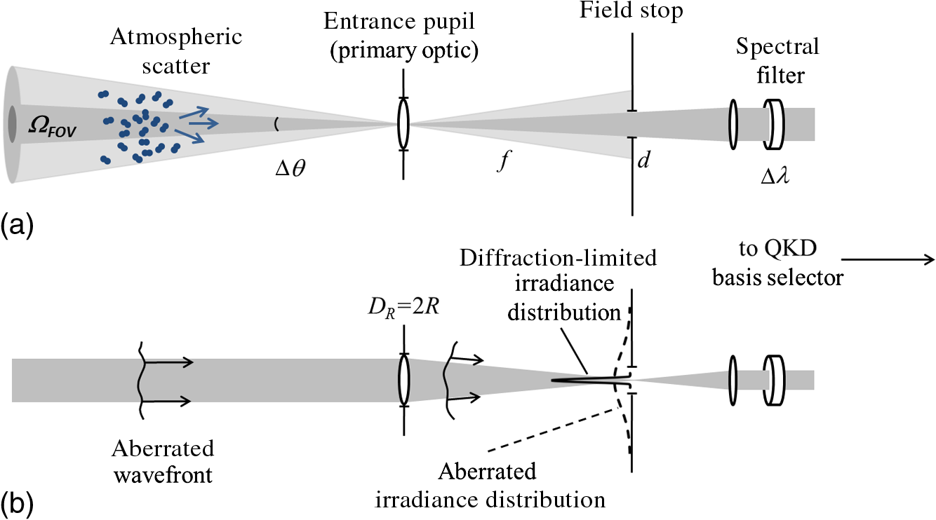 The number of sky-noise photons, , entering the receiver in a detection window is proportional to the sky radiance according to the radiometric expression20 where is the sky radiance in , is the receiver solid-angle FOV, is the radial extent of the primary optic, is the optical wavelength, is the spectral filter bandpass in , is the integration time for photon counting, is Planck’s constant, and is the speed of light. For a given value of the sky radiance, the number of noise photons may be reduced by reducing the spectral bandpass, the temporal gate width, and the receiver FOV.2.2.Atmospheric-Turbulence-Induced AberrationsFigure 1(b) shows the effects of turbulence on signal transmission at the FS. In the absence of aberrations, the primary optic focuses an incident signal to a diffraction-limited irradiance distribution. For a signal photon derived from an attenuated laser pulse, the irradiance distribution represents the photon probability function. For the case of a planar wavefront with uniform amplitude incident upon a circular aperture, the diffraction-limited irradiance distribution at focus is described by the Airy function with a central disk of diameter . Reducing the FS to this diameter passes 84% of the signal while blocking sky noise associated with larger field angles. Reducing the FS further decreases both the transmitted sky noise and the signal. Aberrations increase the size of the signal irradiance distribution at the FS. For atmospheric-turbulence-induced aberrations, the strength of turbulence integrated over a propagation path is characterized by Fried’s coherence length .42 Sarazin and Roddier43,44 computed the angular FWHM of the long-exposure irradiance distribution with turbulence to be approximately . In analogy to the Airy disk, we define the turbulence-induced spot size to be that which captures about 84% of the power. For primary optic diameters larger than , this aberrated spot size at focus is found to be approximately . Relative to the diffraction-limited case, high transmission requires the diameter of the FS to be increased from to . This increases the linear FOV from to and, correspondingly, increases the number of noise photons transmitted by the FS by a factor of . In principle, an AO system can restore the aberrated wavefront to near-diffraction-limited quality. Within the boundaries established by diffraction and turbulence, AO could play a significant role in preserving the transmission of signal photons at reduced FOVs that would substantially reduce background sky noise. The potential benefit of AO to sky noise reduction can be estimated as follows. Atmospheric turbulence is characterized by standard altitude-dependent turbulence profiles. The strength of turbulence is both angle-dependent and wavelength-dependent. For the commonly used turbulence profile,45 henceforth referred to as , and a wavelength of 780 nm, ranges from about 9 to 4 cm for pointing angles ranging from 0 deg to 75 deg from zenith, respectively. For a diameter receiver aperture, the corresponding range of turbulence-limited FOVs is 18 to . In the absence of turbulence, the diffraction-limited FOV is . At 75 deg from zenith, reducing the FOV from the turbulence-limited FOV to the diffraction-limited FOV would reduce sky noise by a factor of 400. Assuming a perfect AO system, this reduction in optical noise could be achieved without increasing the signal loss at the FS. 3.Quantifying the Effects of Turbulence and Adaptive Optics on Photon Capture EfficiencyIn practice, AO does not completely compensate for turbulence-induced aberrations. Limitations occur due to the finite spatial resolution and finite temporal response of the AO system. For a given set of atmospheric parameters and AO system specifications, the optical efficiency of the system can be calculated using numerical methods. In the analysis that follows, it is assumed that the transmission efficiencies associated with classical irradiance distributions represent the transmission probabilities for individual photons from an attenuated laser pulse. It is also assumed that the FS is imaged onto the photodetectors without loss of energy due to vignetting. 3.1.Quantum Key Distribution Receiver with Adaptive OpticsFigure 2 shows a conceptual schematic of an optical receiver that includes both a QKD receiver and an AO system. The AO system architecture is based on systems previously demonstrated.36,37 AO systems require light from either a natural or artificial beacon to probe the atmospheric turbulence.36,37,46 Control signals for the AO system are generated from measurements performed on the aberrated beacon wavefront. In the analysis that follows, it is assumed that the satellite includes both an AO beacon laser and a QKD photon source. The two sources generate copropagating optical pulses that are synchronized in time, but at different wavelengths to allow chromatic separation at the receiver. Fig. 2Schematic illustrating the integration of an AO system with a telescope and QKD receiver. Components include a primary mirror (PM), FSM, DM, DBS, BCSF, BS, FPTS, SHWFS, CPU, M, QCSF, PBS, Geiger-mode APD, and HWP. Control signals are shown as dashed lines. 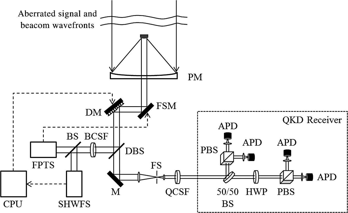 Wavefront errors caused by atmospheric turbulence consist of a tilt component that causes an image to jitter and higher-order spatial components that cause the point spread function to enlarge. Correspondingly, the AO system consists of a fast steering mirror (FSM) that tracks the tilt component of the wavefront error and a deformable mirror (DM) that compensates higher-order wavefront errors. A dichroic beam splitter (DBS) diverts the beacon wavefront to the wavefront sensing system. A beacon-channel spectral filter (BCSF) transmits the beacon wavelength while blocking other spectral components. A beam splitter (BS) transmits a portion of the beacon light to a focal plane tracking sensor (FPTS) that measures the tilt component of the wavefront error and generates control signals for the FSM. The reflected light propagates to a Shack–Hartmann wavefront sensor (SHWFS) that determines the higher-order aberrations and generates control signals for the DM. In a closed-loop AO system, dynamic feedback control reduces residual wavefront errors. The AO system’s dynamic performance limit is characterized by the system bandwidth. Beyond this frequency, the amplitude response of the system is insufficient to be considered useful or stable. The quantum channel wavelength is transmitted by the DBS, reflected by a mirror (M), and brought to a focus at the FS of the system. A quantum-channel spectral filter (QCSF) transmits the quantum-channel wavelength to the QKD receiver while blocking other spectral components. Within the QKD receiver, a 50/50 BS randomly directs photons to the two mutually unbiased measurement bases of the BB84 protocol. In the reflected path, a polarizing beam splitter (PBS) and two gated avalanche photodiodes (APDs) measure the polarization state of the photon in the rectilinear basis. In the transmitted path, a half-wave plate (HWP) rotates the polarization states by 45 deg for measurement in the diagonal polarization basis. 3.2.Numerical Simulation of Propagation Through Turbulence and an Adaptive Optics SystemThe photon capture efficiency associated with turbulence, , is defined to include the turbulence-related losses associated with both transmitter-to-receiver aperture coupling and propagation through the FS of the receiver. Aperture-to-aperture coupling losses due to diffraction are accounted for separately. The term is quantified with a simulation code that includes the effects of turbulence on wave propagation and the effects of a closed-loop AO system within the receiver as shown in Fig. 2. Wave-optics simulations are performed with Atmospheric Compensation Simulation, a simulation code developed by Science Applications International Corporation.40,41 The wave-optics propagation code has been anchored to experimental data and used to anchor other simulation codes.47 The code is based on the principles of scalar diffraction theory. The simulated AO system includes an FPTS and FSM for tilt estimation and correction and an SHWFS and DM for higher-order aberration correction. The hardware emulations include models for the wavefront sensor cameras that include real world effects such as noise, pixel diffusion, and latencies. Simulations are performed for receiver pointing angles ranging from zenith to 75 deg from zenith. For each elevation angle, 20 realizations of atmospheric turbulence are simulated. For each realization of turbulence, the atmosphere is simulated by 10 phase screens distributed throughout the atmospheric path. Each phase screen is a random realization of turbulence consistent with Kolmogorov statistics and the specified turbulence strength profile. Numerical methods based on scalar Fresnel integrals48,49 propagate the optical field from the transmitter through the phase screens50 to the receiving aperture. From there, the optical field is reflected from an FSM and then a DM. These components are simulated in a closed-loop for iterative feedback control. 3.3.Adaptive Optics System ParametersThe FPTS is modeled as a lens and focal plane quadrant detector. The SHWFS is modeled as a element array of lenslets and quadrant detectors. The SHWFS is assumed to be shot-noise limited as is typically the case for systems with cooperative beacons. The DM is modeled as a continuous face sheet driven by a array of actuators. The diameter of the individual lenslets in pupil space is such that is less than unity for the range of turbulence strengths encountered in a atmospheric profile. In stronger turbulence, where exceeds unity, the system performance is degraded.46 In the simulations, the FPTS centroid, SHWFS centroids, and residual wavefront errors are updated at 10 kHz. The FSM and DM are also updated at 10 kHz. The tracking bandwidth is 200 Hz and the bandwidth for higher-order correction is 500 Hz. These system parameters are considered to be within the state of the art. It is assumed that the cooperative beacon on the satellite provides light at 810-nm wavelength for the FPTS and SHWFS. The quantum channel wavelength is assumed to be 780 nm, allowing separation of the two wavelengths. It is further assumed that any beacon light transmitted by the DBS and QCSF is insignificant compared to other noise sources. Applying wavefront correction at a wavelength that is shorter than the beacon wavelength can lead to residual wavefront errors. While these errors are accounted for in the simulations, they are negligible due to the small separation in wavelengths. Similarly, the beacon and quantum-channel pulses are separated in time, but on a timescale over which the atmosphere is static in the simulations. For the purpose of analysis, it is assumed that the satellite travels in either a 400- or 800-km altitude circular orbit. The telescope slews to follow the motion of the satellite. The altitude-dependent wind speed is described by the Bufton wind profile. In order to consider the worst-case scenario, the wind direction is assumed to be opposite to the slew direction, producing the highest Greenwood frequency for a particular turbulence profile. 3.4.Atmospheric Turbulence ParametersThe effects of turbulence on an optical field are characterized by temporal, angular, and spatial coherence parameters. The temporal coherence, given by the Greenwood frequency , is dependent upon the slew rate of the telescope and, therefore, the altitude of the satellite. The angular coherence is given by the isoplanatic angle . The spatial coherence is given by Fried’s coherence length . Greenwood frequencies exceeding the correction bandwidth and isoplanatic angles smaller than the angular subtense of the source result in a degraded performance of the AO system. Rytov is a direct measure of scintillation experienced by the optical field at the receiver entrance pupil. Rytov values greater than about 0.4 indicate deep turbulence where scintillation leads to degradation in the performance of the AO system. In the presence of scintillation, the SHWFS is unable to accurately measure wavefront errors due to intensity nulls in the field. Table 1 shows turbulence parameters calculated at each of the five elevation angles for the two turbulence profiles and two orbit altitudes considered in the analysis that follows. For a 10-cm transmitter aperture, the isoplanatic angles are larger than the angular subtense of the source for all cases. For the 800-km orbit, the Greenwood frequency remains within the 500 Hz AO system bandwidth for all cases shown except 75 deg in turbulence. For the 400-km orbit, the higher slew rates cause the Greenwood frequency to exceed the AO system bandwidth at 75 deg from zenith in turbulence and at all angles shown below zenith in turbulence. At the 75 deg elevation angle, Rytov values indicate deep turbulence conditions. For , the SHWFS subaperture size in pupil space is . In turbulence, is smaller than the subaperture size at the 60 deg and 75 deg elevation angles leading to under-resolved local wavefront tilts. Table 1Turbulence parameters for five elevation angles relative to zenith with 400- and 800-km altitude circular orbit altitudes. Parameters include Fried’s coherence length r0, the isoplanatic angle θ0, Rytov, and the Greenwood frequency fG. Parameters are shown for 1×HV5/7 and 3×HV5/7 turbulence profiles.
3.5.Results: Photon Capture Efficiency Probability DistributionsThe turbulence-related photon capture efficiency is calculated for each elevation angle from the 20 realizations of atmospheric turbulence. For each realization, the simulated AO system iterates to steady state minimizing the wavefront error at the SHWFS. Figure 3 shows sample results presented as probability density functions (PDFs) calculated for turbulence, a receiver aperture size, and a pointing angle at zenith. The transmitter is treated as an unresolved point source relative to a 16-cm grid spacing at the 400-km orbit. Capture efficiencies calculated with tilt correction only are shown in red. Capture efficiencies calculated with the addition of higher-order AO are shown in blue. Since tilt correction is required for tracking the satellite, the case without atmospheric tilt correction is not considered here. Fig. 3Examples of PDFs for the turbulence-related photon capture efficiency calculated for a turbulence profile and a pointing angle at zenith. Results obtained with a FOV are shown for (a) a 400-km altitude circular orbit and, (b) an 800-km altitude circular orbit. Results obtained with a FOV are shown for (c) a 400-km altitude circular orbit and (d) an 800-km altitude circular orbit. Results obtained with tilt correction only are shown in red. Results obtained with the addition of higher-order AO are shown in blue. 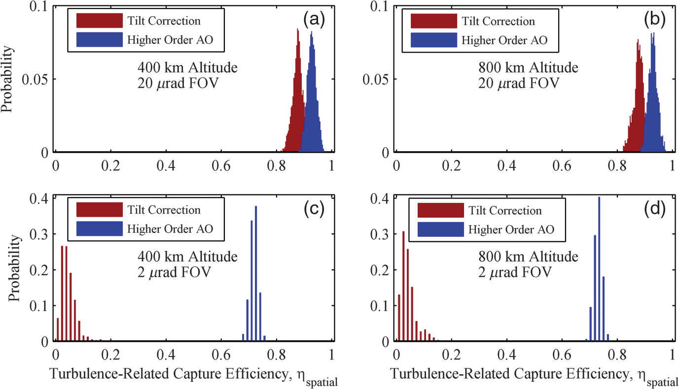 Figures 3(a) and 3(b) show results calculated for a FOV with 400- and 800-km altitude circular orbits, respectively. At this FOV, the mean capture efficiencies increase from 88% with tilt correction alone to 93% with the addition of higher-order AO. Figures 3(c) and 3(d) show the corresponding results calculated for a FOV. At the reduced FOV, turbulence leads to significant losses at the FS. The mean capture efficiencies now increase from only about 5.5% with tilt correction alone to about 73% with the addition of higher-order wavefront compensation. In both cases, the capture efficiency improves measurably with the addition of higher-order AO, but does not reach unity. This is due to the imperfect nature of the AO system and the fact that the small turbulence-related losses that occur in aperture-to-aperture coupling cannot be recovered by any AO system implemented in the receiver. The relative benefit of AO is more significant at the smaller FOV where losses due to turbulence are greater. Increasing the orbit altitude from 400 to 800 km decreases the Greenwood frequency. However, this has a negligible effect on the results since, for the examples shown, all turbulence parameters are within the correction tolerances of the AO system modeled. 4.Secure Key Generation Rates with a Decoy-State Quantum Key Distribution ProtocolThe final measure of effectiveness for a QKD system is the rate at which key bits can be generated in a secure key sharing protocol. Methods for estimating SKG rates in the original BB84 protocol assume that potential information leakage to an eavesdropper can be inferred from the measured QBER and that a privacy amplification algorithm will be implemented to reduce information leakage to meet security criteria.51 An information theoretic upper bound on information leakage determines the fraction of raw key bits to be retained in the secure key. High-loss quantum channels are particularly sensitive to photon-number-splitting (PNS) attacks on multiphoton pulses.52 In the PNS attack, the eavesdropper selectively blocks single-photon pulses where eavesdropping would introduce errors, and retains a photon from multiphoton pulses, allowing the eavesdropper to gain complete knowledge of the bit value without introducing errors. The decoy state protocol was proposed53 and developed54 to address this problem in high-loss channels. The protocol introduces decoy pulses with a mean photon number that is different from that of the signal pulses. Measurements of the decoy pulse detection yield allow the key sharing parties to detect the PNS attack and more accurately estimate possible information leakage from the measured QBER. 4.1.Secure Key Rate Equations for the Vacuum-Plus-Weak-Decoy-State Quantum Key Distribution ProtocolThis section reviews the rate equations for the vacuum-plus-weak-decoy-state QKD protocol implemented via polarization encoding of photons from a Poissonian light source as presented by Ma et al.55 The calculation includes the effects of sky noise, detector dark counts, polarization crosstalk, mean photon number, and photon losses. The SKG rate per signal state, or secret bit yield, is given by where the protocol efficiency is 1/2 for the BB84 protocol, is the mean photon number of the signal states, is the gain of the signal states, is the overall QBER, is the gain of the single-photon states, is the error rate of single photon states, is the bidirectional error correction efficiency, and is the Shannon binary entropy function. The gain of the signal states is given by where is the background detection probability, is the signal detection probability, and is the efficiency of signal photon transmission and detection. The lower bound for the gain of the single-photon states is given by where denotes the mean photon number for the weak decoy state, , and is the gain of the weak decoy state given by substituting for in Eq. (3). The upper bound of is given by where is the lower bound for the yield of the single-photon states given byThe overall QBER associated with signal photons is given by where is the error rate due to noise and is the probability that an incorrect bit value occurred due to polarization crosstalk.The background detection probability is calculated including contributions from sky radiance and detector dark counts where is the probability of detecting a sky-noise photon, is the efficiency of transmission through the spectral filter, is the efficiency of photon detection, and is the efficiency of transmission through the remaining receiver optics.14 The probability of a detection event occurring due to detector noise is , where is the detector dark count rate at each of four identical detectors. The total signal transmission efficiency also includes angle-dependent terms associated with propagation from the transmitter aperture through free-space, including the atmospheric path where is the angle-dependent geometrical coupling efficiency between the transmitter and receiver apertures due to diffraction and finite aperture sizes, is the angle-dependent transmission efficiency associated with atmospheric scattering and absorption,14 and is the angle-dependent transmission efficiency associated with atmospheric turbulence.4.2.Satellite-to-Earth Quantum Channel ParametersSKG rates are calculated with the following parameters assumed: The quantum channel wavelength is for low beam divergence, high atmospheric transmission, and high detector efficiency.14 The beacon channel wavelength is 810 nm. The radial extent of the receiver primary optic is . The spectral filter bandpass and transmission are and , consistent with a commercially available dielectric interference filter.56 The detector efficiency, dark count rate, and gate duration are , , and consistent with the operation of a commercially available Geiger-mode APD.57 The collective optical efficiency of the remaining components in the receiver is . It is assumed that the output of the quantum channel source is expanded to uniformly illuminate the transmitter exit pupil and that all losses incurred by vignetting at the transmitter aperture contribute to the attenuation that is required to achieve the mean photon numbers, and . Under this assumption, it is not necessary to account for losses within the transmitter. For the aperture sizes and propagation ranges considered, the angle-dependent aperture-to-aperture coupling efficiency can be approximated by the Friis equation, , which assumes a uniformly illuminated transmitter aperture.58,59 The diameters of the transmitter and receiver apertures are and , respectively. The propagation distance is calculated as a function of the receiver pointing angle and satellite altitude. For a 400-km altitude circular orbit, propagation distances range from 400 km at zenith to 1175 km at 75 deg from zenith. For an 800-km orbit, the propagation distances range from 800 km at zenith to 2033 km at 75 deg from zenith. The angle-dependent transmission efficiencies are calculated with MODTRAN assuming clear sky conditions. Assumed values range from at zenith to at 75 deg from zenith. In the absence of turbulence-related losses, and the signal transmission efficiencies , expressed in dB of loss, are to 28 dB for the 400-km orbit and 24 to 33 dB for the 800-km orbit. The background detection probability is calculated from Eq. (8) with the number of noise photons calculated from Eq. (1). The gain of the signal state is calculated from Eq. (3) with the signal transmission efficiency calculated from Eq. (9), including contributions from , , and . The signal QBER is calculated from Eq. (7) with the error rate due to noise, , taken to be 1/2 under the assumption the background is random. It should be noted that the polarization distribution of sky radiance has been studied in detail,60 but is not included in this analysis. The probability of a projective polarization measurement in a matched polarization basis yielding an incorrect result due to depolarization in propagation and improper alignment has been measured experimentally in a satellite-Earth optical link.61 The following analysis assumes the reported measured value of . The gain of the single-photon states is calculated from Eq. (4), assuming a decoy-state mean photon number . In order to specify an optimized mean photon number for the signal state, Eq. (2) was evaluated against as a free parameter. The mean photon number was determined to be an optimum value for the parameters assumed here.29 The single-photon error rate is calculated from Eq. (5) with calculated from Eq. (6). The efficiency of error correction is assumed to be a constant value of 1.22, the commonly used value associated with Cascade error correction. 4.3.Results: Secure Key Generation Rate Probability DistributionsThe statistical nature of turbulence leads to statistical distributions of SKG rates. SKG rates are calculated by evaluating Eq. (2) in Sec. 4.1 for statistical distributions of similar to those described in Sec. 3.5. Figures 4(a) and 4(b) show examples of SKG rate PDFs calculated from the capture efficiencies shown in Figs. 3(c) and 3(d), respectively, for the case of a FOV at zenith. This example assumes a turbulence profile and a sky radiance of . In order to present SKG rates in units of secure key bits per second, a system rate of 10 MHz is assumed as a multiplicative factor to Eq. (2). Fig. 4Examples of SKG rate PDFs calculated in the presence of turbulence assuming a receiver with a FOV pointing to zenith, a sky radiance of , a turbulence profile of , a system rate of 10 MHz, and a satellite in a circular orbit at an altitude of (a) 400 km and (b) 800 km. Results obtained with tilt correction alone are shown in red. Results obtained with the addition of higher-order AO are shown in blue. 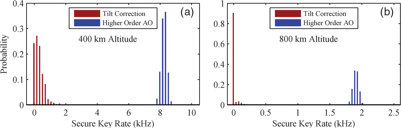 Figure 4(a) shows results calculated for the 400-km altitude orbit. SKG rates with tilt correction alone are shown in red with a distribution around a mean value of 406 Hz. Note that a significant probability exists for a key rate of zero. Introducing higher-order AO results in a significant increase in SKG rates as shown in blue with a distribution around a mean value of 8.3 kHz. Figure 4(b) shows results calculated for the 800-km orbit. With tilt correction alone, the mean SKG rate is only 0.1 Hz, with zero being the most probable key rate. Introducing higher-order AO increases the mean SKG rate to 1.9 kHz. The SKG rates are significantly lower for the 800 km orbit as a consequence of the reduced geometrical capture efficiency at the longer propagation distances. 5.Simulation Results: Daytime Key Rates with Wavefront Tilt Correction and Higher-Order Adaptive OpticsNumerical simulations are performed for turbulence conditions described by and turbulence profiles with receiver elevation angles ranging from zenith to 75 deg from zenith. Sky radiance values of 25 and are considered with receiver FOVs ranging from 0.5 to . The case with tilt correction alone is compared to the case where higher-order AO is also assumed. Results are shown for satellites in 400- and 800-km circular orbits. Figure 5 shows SKG rates calculated for a sky radiance of and a turbulence profile plotted as a function of the receiver FOV. SKG rates are calculated for pointing angles of 0 deg, 30 deg, 45 deg, 60 deg, and 75 deg from zenith and represented in black, green, red, blue, and yellow, respectively. Mean SKG rates are shown as circles and error bars represent one standard deviation in the statistical distributions. The circles are connected by solid lines introduced as an aid to the eye. Results for the case with tilt correction alone are shown in Figs. 5(a) and 5(b). Those calculated with the addition of higher-order AO are shown in Figs. 5(c) and 5(d). Fig. 5SKG rates as a function of the receiver FOV calculated assuming a sky radiance of , a turbulence profile of , and a system rate of 10 MHz. Numerical results are shown for pointing angles of 0 deg, 30 deg, 45 deg, 60 deg, and 75 deg from zenith assuming (a) a 400-km circular orbit with tilt correction, (b) an 800-km circular orbit with tilt correction, (c) a 400-km circular orbit with higher-order AO, and (d) an 800-km circular orbit with higher-order AO. 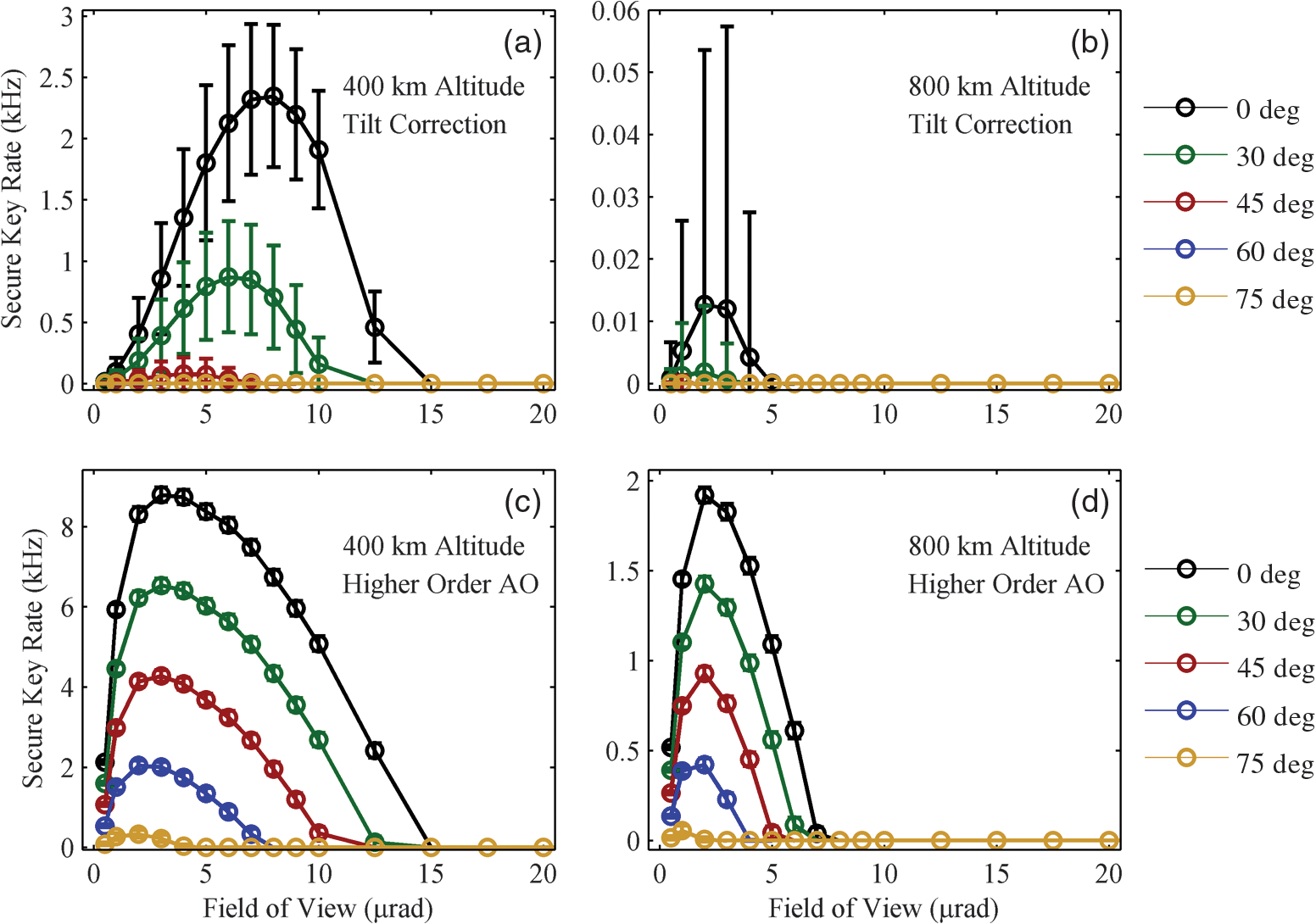 Figure 5(a) shows results for the 400-km orbit with tilt correction. For FOVs larger than , the QBER due to sky noise is sufficiently high to preclude SKG. For FOVs below , sky noise can be reduced sufficiently to allow SKG within 45 deg of zenith. For a given FOV, however, key rates are unstable due to statistical variations in the uncompensated higher-order aberrations. With tilt correction alone, FOVs in the vicinity of 3 to represent the optimum trade-off between noise reduction and signal preservation. With the addition of higher-order AO, shown in Fig. 5(c), stable SKG rates in excess of 1 kHz are possible within 60 deg of zenith. With higher-order AO, the standard deviation in SKG rates can be small relative to the mean value. With higher-order correction, FOVs in the vicinity of 2 to represent the optimum trade-off between noise reduction and signal preservation. Below this range, signal losses reduce key rates even with AO. At a FOV of , the Airy disk would theoretically pass the FS with about 84% power efficiency. Since AO is not perfect, the transmission is lower. Furthermore, the focused irradiance profile at the FS moves as AO iterates, leading to some time-dependent loss variance. Figure 5(b) shows results for the 800-km orbit with tilt correction. For a given elevation angle, the QBER as defined in Eq. (7) has increased due to the increased propagation losses. Consequently, SKG is only possible through further reductions in the FOV and at smaller angles relative to zenith where propagation distances are minimized for a given orbit altitude. Secure key rates in this case are subject to dropouts represented by large error bars relative to the mean value. With the addition of higher-order AO, shown in Fig. 5(d), stable SKG rates in excess of 300 Hz are possible within 60 deg of zenith. As in the case of Fig. 5(c), the standard deviation in SKG rates can be small relative to the mean value. Within each family of curves, SKG rates decline as the elevation angle increases from zenith. This is due to the increased losses that occur with beam divergence over the increased propagation distances and also due to the increased strength of turbulence that occurs with increased atmospheric path length. At 75 deg, the onset of deep turbulence and a high Greenwood frequency result in reduced AO system performance. Figure 6 shows the corresponding results calculated under more challenging conditions; namely, a sky radiance of and a turbulence profile. Results for the case with tilt correction alone are shown in Figs. 6(a) and 6(b). With tilt correction alone, the signal loss due to turbulence at small FOVs is sufficiently high to preclude SKG at all elevation angles considered. SKG rates calculated with the addition of higher-order AO are shown in Figs. 6(c) and 6(d). With higher-order AO, SKG is possible. However, relative to the results shown in Fig. 5(c) and 5(d), the increased sky noise reduces the FOV at which SKG is possible. Fig. 6SKG rates as a function of the receiver FOV calculated assuming a sky radiance of , a turbulence profile of , and a system rate of 10 MHz. Numerical results are shown for pointing angles of 0 deg, 30 deg, 45 deg, 60 deg, and 75 deg from zenith assuming (a) a 400-km circular orbit with tilt correction, (b) an 800-km circular orbit with tilt correction, (c) a 400-km circular orbit with higher-order AO, and (d) an 800-km circular orbit with higher-order AO. 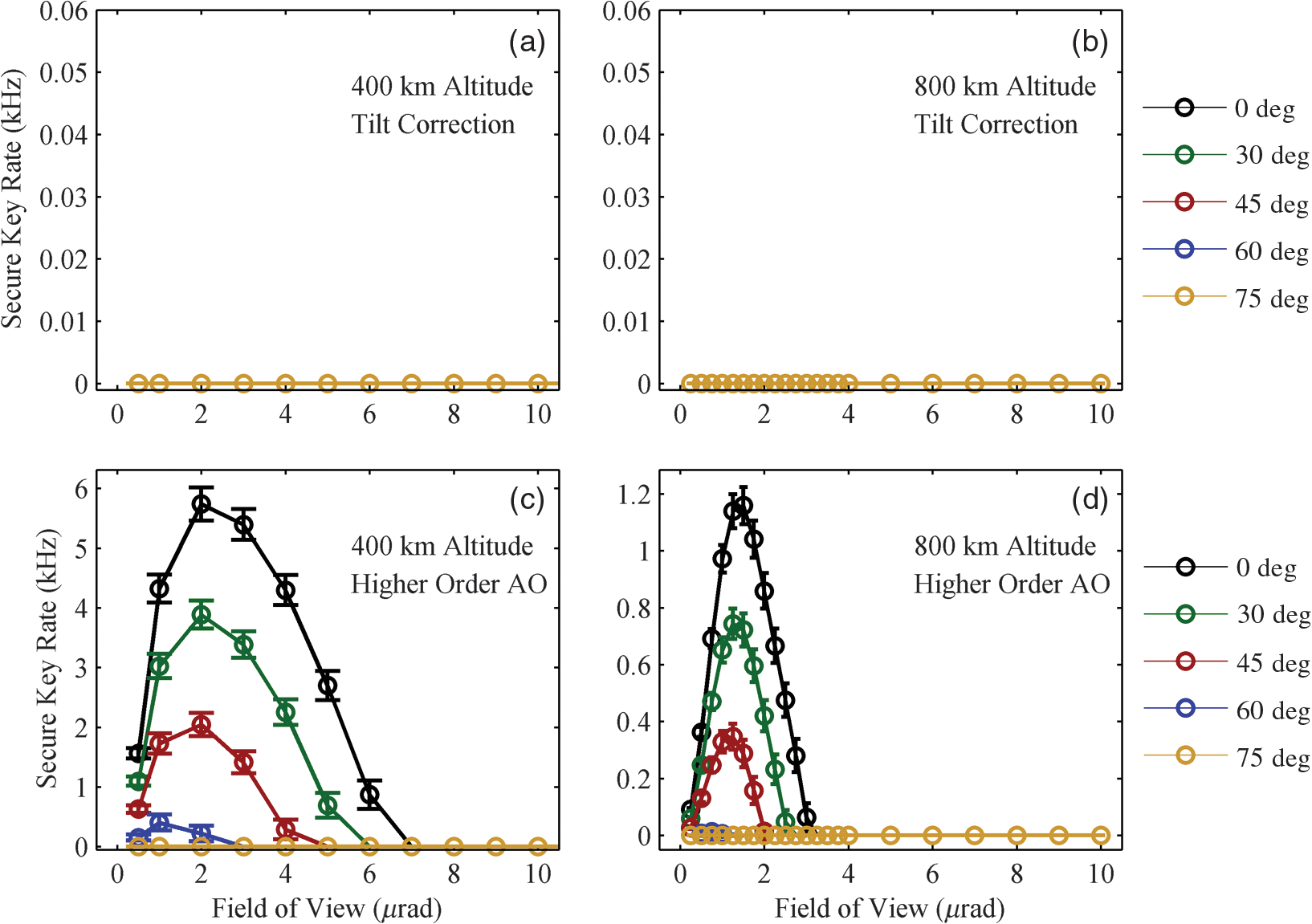 For the case of the 400-km orbit shown in Fig. 6(c), SKG rates in excess of 1 kHz are possible at elevation angles within 45 deg of zenith for FOVs below about . Relative to the results in Fig. 5(c), the factor-of-four increase in requires a factor-of-two decrease in the FOV. Beyond 60 deg elevation angle, the effects of turbulence are stressing the capability of the AO system assumed in this particular simulation. At 60 deg from zenith, the Greenwood frequency, shown in Table 1, is 780 Hz, which is significantly larger than the 500 Hz AO correction bandwidth. At 75 deg from zenith, the Rytov value is 1.19 indicating deep turbulence where scintillation degrades SHWFS performance. At 75 deg, is only 65% of the SHWFS subaperture size, leading to poorly resolved wavefront tilts. The result is a reduced SKG rate at 60 deg and negligible SKG at 75 deg. For the case of the 800-km orbit shown in Fig. 6(d), SKG is only possible at FOVs below . At this altitude, slew rates are lower and Greenwood frequencies are more benign than for the 400-km altitude case. However, the increased propagation distance results in increased losses that negatively impact key rates. SKG rates in excess of 200 Hz are possible within 45 deg of zenith, but rates are negligible beyond 60 deg from zenith. 6.DiscussionAO was demonstrated to be an enabling technology for daytime satellite-to-Earth QKD. The goal in implementing AO in a QKD receiver is to optimize SKG rates by optimizing the noise/loss trade space associated with the receiver FOV. Within a range bounded by turbulence and diffraction, AO is a mature technology for preserving the quantum signal at reduced FOVs. For example, assuming 1× turbulence, a 75 deg angle from zenith, and a perfect AO system, sky noise could be reduced by a factor of 400 without additional signal loss. AO, however, is not perfect. The performance is dependent upon the AO system parameters and the strength of turbulence. Photon capture efficiencies resulting from atmospheric turbulence and a closed-loop AO system were quantified for a specific system with numerical simulations based on Fresnel propagation and AO control theory. Information-theoretic estimates of SKG rates for a decoy-state QKD protocol were calculated based on the simulated capture efficiencies. Results show that in moderate turbulence, simply reducing the receiver FOV to values smaller than previously discussed in the literature can reduce sky noise sufficiently to enable SKG in daylight. The addition of higher-order AO technologies enhances SKG rates considerably and even enables SKG in stronger turbulence where it would otherwise be prohibited as a consequence of background optical noise and signal loss due to turbulence and propagation. Furthermore, higher-order AO improves the stability of SKG rates when turbulence-induced losses are a factor. The relative benefit of AO is more significant at smaller FOVs where losses due to turbulence are greater. The simulation can be applied to modeling the benefits of adaptive spatial filtering with other AO components and other turbulence conditions. Adaptive spatial filtering would likely benefit other QKD protocols and applications involving the transmission of quantum information over free-space channels. Adaptive spatial filtering may be of particular significance since time-bandwidth product considerations associated with Fourier transform and quantum uncertainty relationships limit the extent to which photons can be filtered spectrally and temporally. AcknowledgmentsThe authors gratefully acknowledge important discussions with Earl Spillar and Imelda Atencio (De La Rue). This work was supported by the Air Force Office of Scientific Research. References“Cryptography today,”
(2015) https://www.nsa.gov/ia/programs/suiteb_cryptography/index.shtml October ). 2015). Google Scholar
M. Campagna et al.,
“Quantum safe cryptography and security,”
(2015) http://www.etsi.org/images/files/ETSIWhitePapers/QuantumSafeWhitepaper.pdf November ). 2015). Google Scholar
C. H. Bennett and G. Brassard,
“Quantum cryptography: public key distribution and coin tossing,”
in Proc. of the IEEE Int. Conf. on Computers, Systems, and Signal Processing (IEEE-1984),
175
–179
(1984). Google Scholar
N. Gisin et al.,
“Quantum cryptography,”
Rev. Mod. Phys., 74
(1), 145
–195
(2002). http://dx.doi.org/10.1103/RevModPhys.74.145 RMPHAT 0034-6861 Google Scholar
V. Scarani et al.,
“The security of practical quantum key distribution,”
Rev. Mod. Phys., 81
(3), 1301
–1350
(2009). http://dx.doi.org/10.1103/RevModPhys.81.1301 RMPHAT 0034-6861 Google Scholar
D. Gottesman et al.,
“Security of quantum key distribution with imperfect devices,”
Quantum Inf. Comput., 4
(5), 325
–360
(2004). QICUAW 1533-7146 Google Scholar
H. Inamori, N. Lütkenhaus and D. Mayers,
“Unconditional security of practical quantum key distribution,”
Eur. Phys. J. D, 41 599
–627
(2007). http://dx.doi.org/10.1140/epjd/e2007-00010-4 Google Scholar
W. K. Wootters and W. H. Zurek,
“A single quantum cannot be cloned,”
Nature, 299
(5886), 802
–803
(1982). http://dx.doi.org/10.1038/299802a0 Google Scholar
C. H. Bennett, G. Brassard and J. M. Robert,
“Privacy amplification by public discussion,”
SIAM J. Comput., 17
(2), 210
–229
(1988). http://dx.doi.org/10.1137/0217014 SMJCAT 0097-5397 Google Scholar
N. Lütkenhaus,
“Security against individual attacks for realistic quantum key distribution,”
Phys. Rev. A, 61
(5), 052304
(2000). http://dx.doi.org/10.1103/PhysRevA.61.052304 Google Scholar
B. C. Jacobs and J. D. Franson,
“Quantum cryptography in free space,”
Opt. Lett., 21
(22), 1854
–1856
(1996). http://dx.doi.org/10.1364/OL.21.001854 OPLEDP 0146-9592 Google Scholar
W. T. Buttler et al.,
“Daylight quantum key distribution over 1.6 km,”
Phys. Rev. Lett., 84
(24), 5652
–5655
(2000). http://dx.doi.org/10.1103/PhysRevLett.84.5652 PRLTAO 0031-9007 Google Scholar
J. G. Rarity et al.,
“Ground to satellite secure key exchange using quantum cryptography,”
New J. Phys., 4 82
(2002). http://dx.doi.org/10.1088/1367-2630/4/1/382 NJOPFM 1367-2630 Google Scholar
R. J. Hughes et al.,
“Practical free-space quantum key distribution over 10 km in daylight and at night,”
New J. Phys., 4 43
(2002). http://dx.doi.org/10.1088/1367-2630/4/1/343 NJOPFM 1367-2630 Google Scholar
X. Shan et al.,
“Free-space quantum key distribution with Rb vapor filters,”
Appl. Phys. Lett., 89
(19), 191121
(2006). http://dx.doi.org/10.1063/1.2387867 APPLAB 0003-6951 Google Scholar
T. Schmitt-Manderbach et al.,
“Experimental demonstration of free-space decoy-state quantum key distribution over 144 km,”
Phys. Rev. Lett., 98
(1), 010504
(2007). http://dx.doi.org/10.1103/PhysRevLett.98.010504 PRLTAO 0031-9007 Google Scholar
M. P. Peloso et al.,
“Daylight operation of a free space, entanglement-based quantum key distribution system,”
New J. Phys., 11
(4), 045007
(2009). http://dx.doi.org/10.1088/1367-2630/11/4/045007 NJOPFM 1367-2630 Google Scholar
J. Y. Wang et al.,
“Direct and full-scale experimental verifications towards ground–satellite quantum key distribution,”
Nat. Photonics, 7
(5), 387
–393
(2013). http://dx.doi.org/10.1038/nphoton.2013.89 NPAHBY 1749-4885 Google Scholar
S. Nauerth et al.,
“Air to ground quantum communication,”
Nat. Photonics, 7
(5), 382
–386
(2013). http://dx.doi.org/10.1038/nphoton.2013.46 NPAHBY 1749-4885 Google Scholar
E. L. Miao et al.,
“Background noise of satellite-to-ground quantum key distribution,”
New J. Phys., 7 215
(2005). http://dx.doi.org/10.1088/1367-2630/7/1/215 NJOPFM 1367-2630 Google Scholar
J. M. P. Armengol et al.,
“Quantum communications at ESA: towards a space experiment on the ISS,”
Acta Astronaut., 63
(1–4), 165
–178
(2008). http://dx.doi.org/10.1016/j.actaastro.2007.12.039 AASTCF 0094-5765 Google Scholar
C. Bonato et al.,
“Feasibility of satellite quantum key distribution,”
New J. Phys., 11
(4), 045017
(2009). http://dx.doi.org/10.1088/1367-2630/11/4/045017 NJOPFM 1367-2630 Google Scholar
A. Tomaello et al.,
“Link budget and background noise for satellite quantum key distribution,”
Adv. Space Res., 47
(5), 802
–810
(2011). http://dx.doi.org/10.1016/j.asr.2010.11.009 ASRSDW 0273-1177 Google Scholar
J.-P. Bourgoin et al.,
“A comprehensive design and performance analysis of low earth orbit satellite quantum communication,”
New J. Phys., 15
(2), 023006
(2013). http://dx.doi.org/10.1088/1367-2630/15/2/023006 NJOPFM 1367-2630 Google Scholar
T. Scheidl, E. Wille and R. Ursin,
“Quantum optics experiments using the international space station: a proposal,”
New J. Phys., 15
(4), 043008
(2013). http://dx.doi.org/10.1088/1367-2630/15/4/043008 NJOPFM 1367-2630 Google Scholar
T. Jennewein et al.,
“QEYSSAT: a mission proposal for a quantum receiver in space,”
Proc. SPIE, 8997 89970A
(2014). http://dx.doi.org/10.1117/12.2041693 PSISDG 0277-786X Google Scholar
T. Jennewein et al.,
“The NanoQEY mission: ground to space quantum key and entanglement distribution using a nanosatellite,”
Proc. SPIE, 9254 925402
(2014). http://dx.doi.org/10.1117/12.2067548 PSISDG 0277-786X Google Scholar
J. E. Nordholt et al.,
“Present and future free-space quantum key distribution,”
Proc. SPIE, 4635 116
–126
(2002). http://dx.doi.org/10.1117/12.464085 PSISDG 0277-786X Google Scholar
M. T. Gruneisen et al.,
“Modeling daytime sky access for a satellite quantum key distribution downlink,”
Opt. Express, 23
(18), 23924
(2015). http://dx.doi.org/10.1364/OE.23.023924 OPEXFF 1094-4087 Google Scholar
I. Capraro et al.,
“Free space quantum key distribution system with atmospheric turbulence mitigation by active deformable mirror,”
in Int. Conf. on Quantum Information,
(2008). Google Scholar
A. Carrasco-Casado, N. Denisenko and V. Fernandez,
“Correction of beam wander for a free-space quantum key distribution system operating in urban environment,”
Opt. Eng., 53
(8), 084112
(2014). http://dx.doi.org/10.1117/1.OE.53.8.084112 Google Scholar
M. T. Gruneisen et al.,
“Adaptive spatial filtering for daytime satellite quantum key distribution,”
Proc. SPIE, 9254 925404
(2014). http://dx.doi.org/10.1117/12.2071278 PSISDG 0277-786X Google Scholar
H. W. Babcock,
“The possibility of compensating astronomical seeing,”
Publ. Astron. Soc. Pac., 65
(386), 229
–236
(1953). http://dx.doi.org/10.1086/126606 PASPAU 0004-6280 Google Scholar
J. W. Hardy, J. Feinleib and J. C. Wyant,
“Real time phase correction of optical imaging systems,”
in OSA Topical Meeting on Optical Propagation through Turbulence,
(1974). Google Scholar
R. W. Duffner, The Adaptive Optics Revolution, A History, 41
–64 University of New Mexico Press, Albuquerque, New Mexico
(2009). Google Scholar
R. Q. Fugate et al.,
“Two generations of laser-guide-star adaptive-optics experiments at the Starfire Optical Range,”
J. Opt. Soc. Am. A, 11
(1), 310
–324
(1994). http://dx.doi.org/10.1364/JOSAA.11.000310 JOAOD6 0740-3232 Google Scholar
R. K. Tyson, Principles of Adaptive Optics, 53
–255 Academic Press, London, UK
(1991). Google Scholar
D. P. Greenwood,
“Bandwidth specifications for adaptive optics systems,”
J. Opt. Soc. Am., 67 390
–392
(1977). http://dx.doi.org/10.1364/JOSA.67.000390 JOSAAH 0030-3941 Google Scholar
D. J. Link,
“Comparison of the effects of near-field and distributed atmospheric turbulence on the performance of an adaptive optics system,”
Proc. SPIE, 2120 87
–94
(1994). http://dx.doi.org/10.1117/12.177701 PSISDG 0277-786X Google Scholar
D. J. Link,
“Simulation of laser guidestar adaptive optics systems,”
Proc. SPIE, 2375 30
–40
(1995). http://dx.doi.org/10.1117/12.207004 PSISDG 0277-786X Google Scholar
D. L. Fried,
“Optical resolution through a randomly inhomogeneous medium for very long and very short exposures,”
J. Opt. Soc. Am., 56 1372
–1379
(1966). http://dx.doi.org/10.1364/JOSA.56.001372 JSDKD3 Google Scholar
F. Roddier,
“The effects of atmospheric turbulence in optical astronomy,”
Progress in Optics, XIX 281
–376 North-Holland(1981). Google Scholar
M. Sarazin and F. Roddier,
“The ESO differential image motion monitor,”
Astron. Astrophys., 227 294
–300
(1990). AAEJAF 0004-6361 Google Scholar
R. K. Tyson, Principles of Adaptive Optics, 29
–31 Academic Press, London, UK
(1991). Google Scholar
R. Q. Fugate,
“Adaptive optics,”
Handbook of Optics Volume III, 1.3
–1.52 2nd Ed.McGraw-Hill, New York, New York
(2001). Google Scholar
“WaveTrain anchoring and validation,”
(2015) https://mza.com/doc/wavetrain/anchor/index.htm December ). 2015). Google Scholar
J. D. Schmidt, Numerical Simulation of Optical Wave Propagation with Examples in MATLAB®, 1
–195 SPIE, Bellingham, Washington
(2010). Google Scholar
D. G. Voelz, Computational Fourier Optics: a MATLAB® Tutorial, 1
–229 SPIE, Bellingham, Washington
(2011). Google Scholar
M. C. Roggemann and B. M. Welsh, Imaging Through Turbulence, 104
–119 CRC Press, New York, New York
(1996). Google Scholar
C. H. Bennett et al.,
“Experimental quantum cryptography,”
J. Cryptol., 5 3
–28
(1992). http://dx.doi.org/10.1007/BF00191318 JOCREQ 0933-2790 Google Scholar
G. Brassard et al.,
“Limitations on practical quantum cryptography,”
Phys. Rev. Lett., 85
(6), 1330
–1333
(2000). http://dx.doi.org/10.1103/PhysRevLett.85.1330 PRLTAO 0031-9007 Google Scholar
W. Y. Hwang,
“Quantum key distribution with high loss: toward global secure communication,”
Phys. Rev. Lett., 91
(5), 057901
(2003). http://dx.doi.org/10.1103/PhysRevLett.91.057901 PRLTAO 0031-9007 Google Scholar
H. K. Lo, X. Ma and K. Chen,
“Decoy state quantum key distribution,”
Phys. Rev. Lett., 94
(23), 230504
(2005). http://dx.doi.org/10.1103/PhysRevLett.94.230504 PRLTAO 0031-9007 Google Scholar
X. Ma et al.,
“Practical decoy state for quantum key distribution,”
Phys. Rev. A, 72
(1), 012326
(2005). http://dx.doi.org/10.1103/PhysRevA.72.012326 Google Scholar
H. T. Friis,
“Introduction to radio and radio antennas,”
IEEE Spectr., 8
(4), 55
–61
(1971). http://dx.doi.org/10.1109/MSPEC.1971.5218045 IEESAM 0018-9235 Google Scholar
S. B. Alexander, Optical Communication Receiver Design, 37 SPIE, Bellingham, Washington
(1997). Google Scholar
N. J. Pust and J. A. Shaw,
“Wavelength dependence of the degree of polarization in cloud-free skies: simulations of real environments,”
Opt. Express, 20
(14), 15559
–15568
(2012). http://dx.doi.org/10.1364/OE.20.015559 OPEXFF 1094-4087 Google Scholar
M. Toyoshima et al.,
“Polarization measurements through space-to-ground atmospheric propagation paths by using a highly polarized laser source in space,”
Opt. Express, 17
(25), 22333
–22340
(2009). http://dx.doi.org/10.1364/OE.17.022333 OPEXFF 1094-4087 Google Scholar
BiographyMark T. Gruneisen is the principal investigator for quantum key distribution research at the Air Force Research Laboratory’s Directed Energy Directorate. He is a fellow of SPIE, chair for the SPIE Quantum Information Science and Technology Conference, and corecipient of the SPIE 2004 Rudolf Kingslake Medal. He received his PhD in optics from the University of Rochester, Rochester, New York, in 1988. Brett A. Sickmiller is an optical research analyst working for Leidos supporting optical and quantum communications research in the Air Force Research Laboratory’s Directed Energy Directorate. He received his PhD in engineering physics from the University of Virginia, Charlottesville, Virginia, in 2008. Michael B. Flanagan is an optical research analyst with Leidos. He earned his doctorate in applied mathematics in 2002 at Texas A&M University and has 11 years’ experience in the field of AO. James P. Black is a senior optical engineer with The Boeing Company. He supports optical and quantum communications research in the Air Force Research Laboratory’s Directed Energy Directorate. |
|||||||||||||||||||||||||||||||||||||||||||||||||||||||||||||||||||||||||||||||||||||||||||||||||||||||||||||||||||||||||||||


