Design and optimization for total internal reflection collimators based on slope-error tolerance analysis

Tao Luo; Gang Wang

doi:10.1117/1.OE.55.2.025103

2 February 2016 Design and optimization for total internal reflection collimators based on slope-error tolerance analysis

Tao Luo, Gang Wang

Author Affiliations +

Optical Engineering, Vol. 55, Issue 2, 025103 (February 2016). https://doi.org/10.1117/1.OE.55.2.025103

Abstract

This work provides a design and optimization method for total internal reflection (TIR) lenses based on slope-error tolerance analysis. This work focuses on how the slope error impacts the central luminous intensity (CLI) of a TIR lens. The concentration standard index (CSI) is introduced as a metric for analyzing the CLI, both locally and globally. A unique design method for improved manufacturing tolerance is introduced, and a way of optimizing the TIR lens design in order to achieve a better slope-error tolerance is presented by evaluating the CSI. Using the design method, a TIR lens is fabricated and this theoretical approach is then demonstrated by a comparison between the tested contours of the TIR surfaces.

1. Introduction

Collimating optics has been widely used in light-emitting diode (LED) lighting to generate light beams with small beam angles and high central luminous intensities (CLIs). As the luminance of LEDs is low compared with some discharge luminaries, it is acceptable to sacrifice some luminous coupling efficiency in order to guarantee a sufficient amount of luminous intensity in ultracompact devices in many applications, and we can refer to this as the “maximized luminous intensity problem,” for which CLI is regarded as the primary attribute of interest.¹

The total internal reflection (TIR) lens is one of the most widely used collimating optical devices for small beam angles and high CLIs; it has several desirable features such as a high concentration ratio with respect to its compact volume, a vast amount of design freedom, and a convenient manufacturing process for mass production.²^,³ Previous work on TIR lenses has focused on producing novel designs, optimizing performance (in terms of efficiency and viewing angle⁴^–⁸), achieving a uniform irradiance distribution,⁸^–¹⁰ and achieving a uniform color distribution.¹¹ Optimizations of initial parameters for better efficiency and CLI with different extended light sources were reported by Chen,¹² and the effects of an extended LED light source on the efficiency and CLI of TIR lenses were studied by Chen¹² and Kari et al.³

In fact, there is an extreme of the CLI, as every infinitesimal surface on the exit pupil has no more than a single ray emitting toward the center as a result of luminance conservation and Etendue conservation. In theory, it is not complicated to achieve the maximum CLI by the methods recommended by Parkyn, Shen, and Chen,¹³^–¹⁶ as each ray from the center of the LED was designed to emit in the collimation direction so that the luminous intensity always reaches the maximum theoretical value for a light source of any size. As a result, it is not theoretically difficult to optimize the CLI in the design stage. However, manufacturing tolerance is very weak in collimators with high concentration ratios. For this reason, manufacturing tolerance has become an important obstacle in achieving impressive TIR lenses with high CLI and the most compact sizes. Deviations in the manufacturing process may result in installation errors and manufacturing defects of the optical surface; this has been discussed by González-Montes et al.¹⁷ However, slope error, when compared to position error, is the main influence on manufacturing tolerance,¹⁸ and should be considered in the design stage. Until now, there have been no quantitative analyses concerned with how the slope-error distribution impacts the performance of certain LED collimators.⁷^,¹⁰^,¹⁷

This paper provides another perspective on TIR lenses designed for concentrators with high concentration ratios from the perspective of manufacturing tolerance. More specifically, this characterization of TIR lenses focuses on the impact of slope error upon the CLI. An analysis of slope-error tolerance is presented; this is followed by a discussion of the ways in which the TIR lens can be optimized to achieve a better slope-error tolerance.

2. Slope Error Problems in Total Internal Reflection Lenses

2.1.

Total Internal Reflection Lenses Structure

Although different structures have been employed in TIR lenses, ⁴^–¹¹ all TIR lenses are designed with mutual groups of surfaces, as shown in Fig. 1. One of the groups includes two refracted surfaces (i.e., surface 1 and surface 2), which aim to focus rays emitted from around the optical axis of the LED into the collimation direction. The other group includes three surfaces: the incident surface to the light source located along the side of the lens, which is called the side incident surface (i.e., surface 3), the TIR surface (i.e., surface 4), and the exit surface (i.e., surface 5). Rays are divided into two categories, depending on which group of surfaces they encounter. The shape of every surface has a high degree of design freedom.

Fig. 1

A sketch of a TIR lens. The lens is made up of two groups of surfaces. The starting points of the side incident surface and the TIR surface are $n_{0}$ and $w_{0}$ , respectively. The tilt angle of the side incident surface is $α$ , and the diameter of the exit pupil is $Φ_{exit}$ . Rays emitted from different groups of surfaces are also plotted.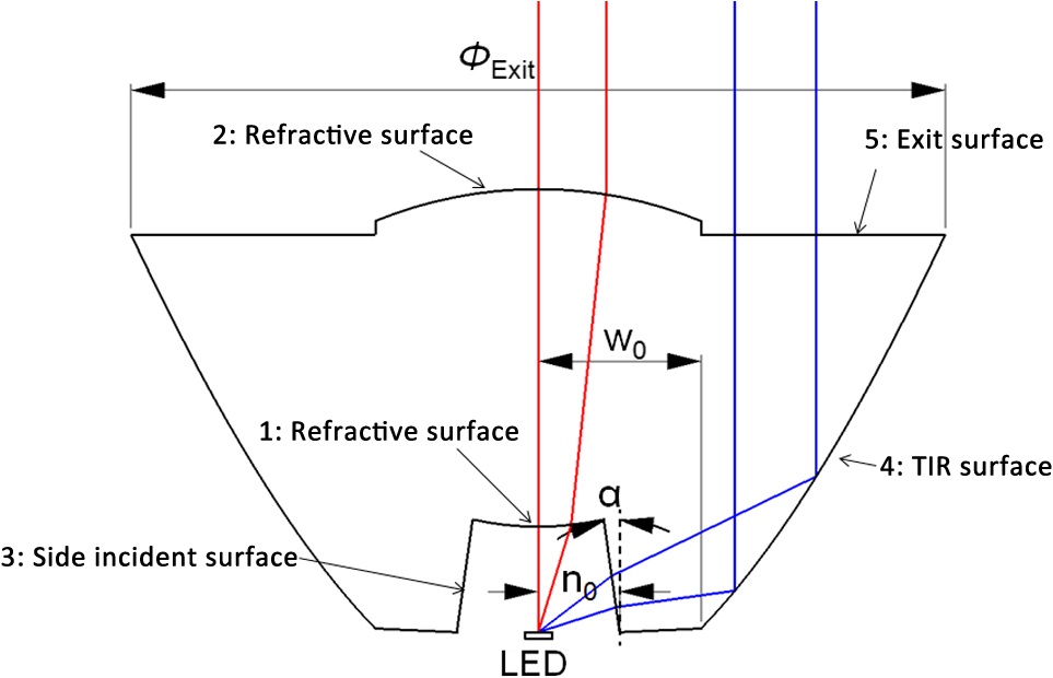

2.2.

Analysis Model of Total Internal Reflection Lenses

According to the error transfer theory described by Winston et al.,¹⁹ it is evident that the two refracted surfaces cause much smaller beam deviations with the same slope errors than the other groups of surfaces because of the small error multiplier values they are associated with. For the same reason, the slope tolerance of the side incident surface and the exit surface is relatively higher than that of the TIR surface. For all of these reasons, the optimizations in this work only focus on the design of TIR surfaces. Without loss of generality, the exit surface (i.e., surface 5) is treated as a plane that is parallel to the $x$ -axis.

Furthermore, the slope error occurs in two dimensions, one dimension is the meridian plane and the other is nonmeridional.²⁰ As the slope error distribution other than that in the meridian plane may be complicated and it can be corrected by molding design and injection technologies without necessarily optimizing the optical designs, we only analyze the slope error in the meridian plane in this work to focus attention on the optical design and optimization for TIR collimators.

Finally, although the luminance is not uniform for real LEDs, we assume the Lambertian distribution in this study to focus our attention on the designs and the lens structures.

2.3.

Central Luminous Intensity Decrease Mechanics

The beam deviation caused by slope error can be analyzed by cone theory. If a “maximized luminous intensity problem” is considered, as the rays impinging toward the center do not deviate when exiting from the plane exit surfaces, the exit surface is not taken into consideration as it does not impact the slope error tolerance characteristics. As a result, the mechanism by which the CLI decreases as a result of slope error is shown in Fig. 2. If slope error increases so that rays “leak” from the cone angle, there is not a single ray impinging toward the collimation direction, and the CLI in this case becomes zero.

Fig. 2

A sketch of the mechanism by which the CLI decreases as a result of slope error. (a) The ray from the center of the LED to the collimation direction as designed. (b) Some other rays will travel toward the collimation direction when the small slope error occurs. (c) Slope error increases to a certain “leakage” from the cone angle with slope error $> 0$ . (d) Slope error increases to a certain “leakage” from the cone angle with slope error $< 0$ .

2.4.

Concentration Standard Index

We propose an evaluation method based on an index referred to as the general concentration standard index (GCSI) for LED collimating optical systems as follows:

Eq. (1)

GCSI (θ, ϕ) = \frac{I (θ, ϕ)}{I_{\max} (θ, ϕ)},

where

I (θ, ϕ)

is the luminous intensity in the direction

(θ, ϕ)

and

I_{\max} (θ, ϕ)

are the maximum values.

The GCSI can be used both in simulations and for experimental testing; furthermore, it is valid for evaluating entire surfaces as well as local, specific positions. For local optical surfaces, the local GCSI ( ${GCSI}_{L}$ ) can be evaluated as the energy utilization toward the target direction of a local surface compared to the extremes of the same surface, which is formulated as

Eq. (2)

{GCSI}_{L} (θ, ϕ, X) = \frac{L_{l} (θ, ϕ, X)}{L_{l, \max} (θ, ϕ, X)},

where

L_{l} (θ, ϕ, X)

is the luminance of the infinitesimal surface at point

X

toward direction

(θ, ϕ)

, and the

L_{l, \max} (θ, ϕ, X)

is the maximum luminance for the same point.

When we consider the “maximized luminous intensity problem,” only the CLI should be considered so that the ${GCSI}_{L}$ is simplified to the local concentration standard index ( ${CSI}_{L}$ ) in that

Eq. (3)

{CSI}_{L} (X) = {GCSI}_{L} (0,0, X) = L_{l} (X) / L_{l, \max} (X),

where

L_{l} (X)

is the luminance contributed by the local TIR surface

X

toward the central direction, and the

L_{l, \max} (X)

is the maximum value of the

L_{l} (X)

.

For a uniform luminance distribution, the maximum CLI contributed by a local surface with area $d S$ can be further derived from Fig. 2 for the Lambertian sources as

Eq. (4)

I_{L} = {\begin{cases} ϕ / π (d S / A_{1}) M_{L} L_{s} & (r_{{PE}_{1}} < U_{0} < r_{{PE}_{2}}) \\ 0 & (else) \end{cases},

where

ϕ

is the luminous flux of the light source,

A_{1}

is the area of the light source,

M_{L}

is the transmission efficiency,

L_{s}

is the luminance of the ray actually impinging to the collimation direction, and

r_{{PE}_{1}}

and

r_{{PE}_{2}}

are two edge rays formed by the light source.

We can hypothesize a limitation of this calculation, referred to as “equal luminance condition I” ( ${ELC}_{1}$ ), whereby the luminance of the LED and the Fresnel losses are equal for all rays inside the same cone angle. In fact, ${ELC}_{1}$ can be always fulfilled for collimator problems with high concentration ratios because the transmission efficiency difference between the angles subtended by incident rays inside the cone angle and the side incident surface are negligible. The ${CSI}_{L}$ can be simplified from Eq. (3) with ${ELC}_{1}$ as follows so that:

Eq. (5)

{CSI}_{L} = I_{L} / I_{L, \max} = {\begin{cases} 1 & (r_{{PE}_{1}} < U_{0} < r_{{PE}_{2}}) \\ 0 & (else) \end{cases},

where

I_{L}

is the CLI contributed by the local TIR surface, and

I_{L, \max}

is the maximum value of the CLI for the same surface.

3. Concentration Standard Index Calculations of Total Internal Reflection Lenses

The calculation of the CSI for a TIR surface follows the steps list below:

1. Cone angle derivation from the shape of the LED light source and TIR surface.
The cone angle is only determined by $r_{{PE}_{1}}$ and $r_{{PE}_{2}}$ , which are reflected by the edge ray from $R_{1}$ $(- R_{0}, 0, 0)$ and $R_{2}$ $(R_{0}, 0, 0)$ , as shown in Fig. 2(a). $R_{th} (x)$ and $L_{th} (x)$ are depicted as the right and left thresholds of the cone angle with the horizontal coordinate $x$ on the TIR surface curve. It also can be viewed as the pin hole image width projected from position $x$ . The values of $R_{th} (x)$ and $L_{th} (x)$ can be expressed as follows:
Eq. (6)
$L_{th} (x) = \frac{1}{2} \vec{r_{{PE}_{1}}}^\vec{r_{PC}} = - \frac{1}{2} ∠ {CPE}_{1} R_{th} (x) = \frac{1}{2} \vec{r_{{PE}_{2}}}^\vec{r_{PC}} = \frac{1}{2} ∠ {CPE}_{2},$
where the minus sign of $L_{th} (x)$ indicates that the angle subtended with the $x$ -axis is greater than $π / 2$ .
2. ${CSI}_{L}$ at local surface
We assume that the slope-error probability distribution follows a normal distribution $Δ S (s)$
Eq. (7)
$Δ S (s) = \frac{1}{\sqrt{2 π} σ} e^{- \frac{{(s - u)}^{2}}{2 σ^{2}}},$
where $s$ is the slope error of the local surface, $μ$ represents the fixed slope error which is mostly a consequence of the injection of plastic process, and $σ$ is the standard deviation of the normal distribution.
With ${ELC}_{1}$ , we can derive the expected value of ${CSI}_{L}$ from Eqs. (5) and (7) along the TIR curve with different horizontal coordinates $x$ with the help of Eq. (8) as follows:
Eq. (8)
${CSI}_{L} (x) = \int_{L_{th} (x)}^{R_{th} (x)} \frac{1}{\sqrt{2 π} σ} e^{- \frac{{(s - u)}^{2}}{2 σ^{2}}} d s .$
3. CSI of the whole surface
Considering the rotational symmetry of the TIR lens, according to Eq. (5) the relationship between the CLI of an entire surface (CSI) and its local value ( ${CSI}_{L}$ ) is
Eq. (9)
$CSI = \frac{\int_{x_{start}}^{x_{end}} {CSI}_{L} (x) L (x) d S}{\int_{x_{start}}^{x_{end}} L (x) d S} = \frac{\int_{x_{start}}^{x_{end}} {CSI}_{L} (x) L (x) \cdot 2 π x d x}{\int_{x_{start}}^{x_{end}} L (x) \cdot 2 π x d x} = \frac{\int_{x_{start}}^{x_{end}} {CSI}_{L} (x) L (x) \cdot x d x}{\int_{x_{start}}^{x_{end}} L (x) \cdot x d x} .$

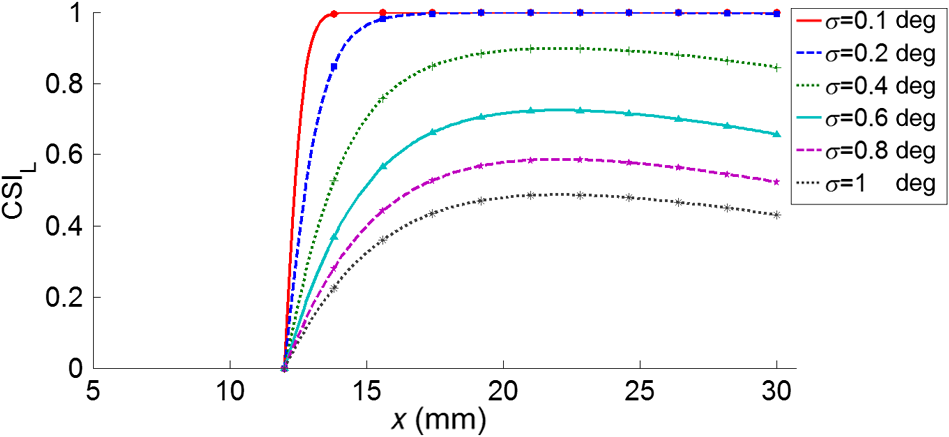
4. Total Internal Reflection Design for Improved Manufacturing Tolerance

With traditional design methods, the TIR surface has always been designed based on the differential geometry method, so that every ray emitted from the center of the light source must be cast to the center to contribute to the CLI.¹³^,¹⁵ We will refer to this as the “point source method.” The angle subtended by $r_{{PE}_{1}}$ and $r_{PC}$ is not necessarily equal to that subtended by $r_{{PE}_{2}}$ and $r_{PC}$ , as shown in Fig. 2(a).

We proposed an edge ray method in this paper which states that the edge rays of the light source $R_{1}$ and $R_{2}$ are considered according to the edge ray principle. The normal of every point along the TIR curve is determined so that the center of the elliptical bundle will be reflected to the collimation direction, as shown in Fig. 3, whereas in the traditional method, the ray is reflected from the center of the light source to the collimation direction.

Fig. 3

A sketch of the edge ray method of optimizing the tolerance for a TIR surface. The initial parameters include the tilt angle of the cross-section of the side incident surface (the inner curve) $α$ ; the distance from the bottom of the inner curve to the center $n_{0}$ ; the $x$ coordinate of the starting point of TIR curve $w_{0}$ ; the diameter of the exit pupil of the collimator 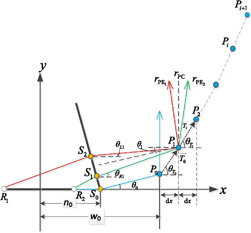$Φ_{exit}$ .

According to the modified design method, the angle between $r_{{PE}_{1}}$ and $r_{{PE}_{2}}$ is constant for the same point $P$ on the TIR curve with the same light source and side incident surface. As the ${CSI}_{L}$ has a maximum value when the absolute values of $R_{th} (x)$ and $L_{th} (x)$ are equal, so that the lens designed by the modified method has an optimized slope-error tolerance. Later in this paper, the analysis is based on the edge ray method in this section, without any special instructions.

5. Results and Discussion

The slope error in the tolerance analysis in the meridian plane consists of two components: fixed slope error and stochastic slope error. The fixed slope error can be formed either by shrinkage during the molding process or by B-spline fitting.¹⁶ On the other hand, stochastic slope error is always caused during the process of manufacturing and is difficult to eliminate from mass production.²¹ Considering the complexity of the program, the TIR surface is designed with a 0.1-mm $x$ -coordinate increment of adjacent points. Later in this paper, we assume a fixed error of $μ = 0$ to focus our analysis on the optical designs with optimized parameters.

We also hypothesize another limitation, referred to as “equal luminance condition II” ( ${ELC}_{2}$ ), whereby the luminance of the LED and the Fresnel losses of the lens are comparatively equal for all rays impinging to the side incident surface. According to physical optics theory, the Fresnel loss is approximately a constant when the incident angle is less than Brewster’s angle. As a large Fresnel loss can induce large dispersed rays and energy loss, it should be eliminated during design procedure.²² In this work, we assume that when the maximum angle between the incident rays of the LED and the normal of the side incident surface does not exceed 62 deg, ${ELC}_{2}$ is always fulfilled, and $L (x)$ in Eq. (9) is always a constant, and we have

Eq. (10)

CSI = \frac{\int_{x_{sta rt}}^{x_{end}} {CSI}_{L} (x) \cdot x d x}{\int_{x_{start}}^{x_{end}} x d x} = 2 \frac{\int_{x_{start}}^{x_{end}} {CSI}_{L} (x) \cdot x d x}{x_{end}^{2} - x_{start}^{2}},

where

x_{start}

and

x_{end}

are the

x

-coordinates of the starting point and the terminal point of the TIR curve, respectively.

5.1.

Slope-Error Tolerance of the Total Internal Reflection Surface

Here we discuss the tolerance of a typical TIR lens. The tilt angle of the lens $α = 8 \deg$ , $n_{0} = 6 mm$ , $w_{0} = 12 mm$ , the diameter of exit pupil $Φ_{exit} = 60 mm$ , and the radius of the LED $R = 1 mm$ . The ${CSI}_{L}$ with different values of slope-error standard deviation $σ$ is also plotted in Fig. 4. The result shows that ${CSI}_{L}$ is not equal to 1 anywhere if the slope-error standard deviation is larger than 0.4 deg.

Fig. 4

The ${CSI}_{L}$ with different values for the slope-error standard deviation $σ$ .

It is not complicated to derive the CSI of the entire TIR surface by Eq. (10) when ${ELC}_{2}$ is fulfilled. Figure 5 shows a CSI comparison between different design methods. The LED with a radius of $R = 3 mm$ is also discussed. The CSI decreases rapidly with a standard deviation $σ$ in the range of 0.3 deg to 0.8 deg with an $R = 1 mm$ light source. Even a stochastic slope error of 0.5 deg will induce 30% degradation in the CLI, which reveals a significant possibility for the loss of luminous intensity in mass production. For a larger light source, the CSI performance is much better due to the larger cone angle formed by the light source. We can see that there should be more concern for the manufacturing tolerance in collimating devices with a small light source.

Fig. 5

CSI with different design methods. The red and green lines designate the edge ray method, whereas the blue and pink lines designate the point source method. LEDs with radii of 1 and 3 mm are also compared.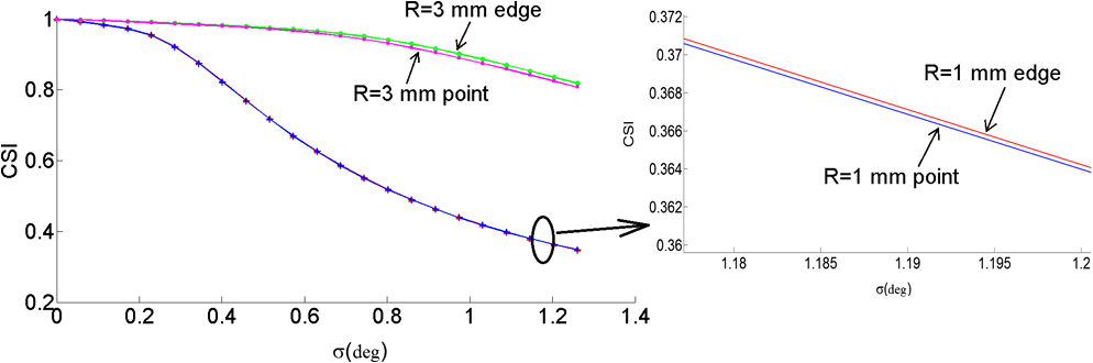

The results also reveal that the edge ray method shows improved slope-error tolerance, although the difference is very small for the case of an LED whose radius is only 1/30 the size of the exit pupil aperture.

5.2.

Optimization for Better Slope-Error Tolerance

We further optimized the parameters for slope-error tolerance; such optimization has been performed in the context of design performance¹² and size effect (which is defined as the reliability of point source approximations in compact LED lens designs) in simulations.³ In this paper, the parameters which have been illustrated in Sec. 4 were optimized. A constraint upon the optimization is ${ELC}_{2}$ , and the results are abandoned when this condition cannot be fulfilled.

5.2.1.

Optimization of the total internal reflection curve with a conical inner surface

In this section, the inner curve is a line. Figure 6 shows the CSI of the TIR surface with different tilt angles at the same starting points for both the inner curve and the TIR curve. The tilt angle ranges from 0 deg to 20 deg, with the same standard deviation of the stochastic slope error of $σ = 0.2 \deg$ . The results show that there is little difference in the CSI with different tilt angles, although a tilt angle around 10 deg yields slight improvements and we can design the tilt angle according to considerations of manufacturing convenience and Fresnel losses.

Fig. 6

CSI of the TIR surface with different tilt angles for the inner curve. The standard deviation of the stochastic slope error of 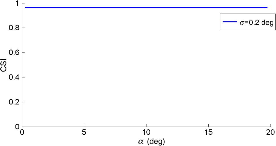$σ = 0.2 \deg$ .

Figure 7(a) shows a diagram of the ${CSI}_{L}$ with a different starting point $n_{0}$ for the inner curve, where the starting point of the TIR curve $w_{0}$ is 12 mm. Figure 7(b) shows the CSI with different values of $n_{0}$ . The results show that a smaller base diameter for the inner curve can yield a better CSI. The optimized starting point occurs around 3 mm.

Fig. 7

(a) ${CSI}_{L}$ and (b) CSI with different starting points for the inner curve, and with a starting point for the TIR curve of $w_{0} = 12 mm$ . The standard deviation $σ$ is 0.2 deg.

Figure 8 shows the impact of different starting points for the TIR curve on the CSI, with a starting point of $n_{0} = 6 mm$ for the inner curve. We can see from Fig. 8(a) that when the starting point is near the light source, the ${CSI}_{L}$ at the bottom is better although it sharply decreases at the end. The optimal starting point occurs around $w_{0} = 10.2 mm$ , as shown in Fig. 8(b).

Fig. 8

(a) ${CSI}_{L}$ and (b) CSI with different starting points for the TIR curve $w_{0}$ , and with a starting point of $n_{0} = 6 mm$ for the inner curve. The standard deviation $σ$ is 0.2 de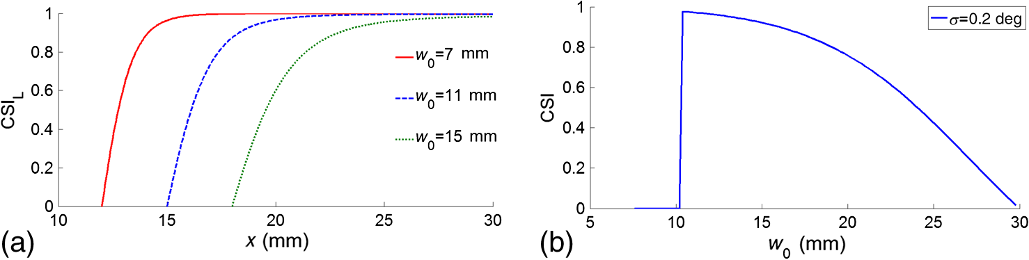g.

We can optimize the starting point of both the inner curve and the TIR curve, as shown in Fig. 9. For the $x$ - and $y$ -coordinates, we calculate the CSI for these parameters every 0.2 mm in order to optimize the performance. A standard deviation of $σ = 0.2 \deg$ is chosen. From the results of Fig. 13, the optimal starting point appears to be (9.2, 10.2).

Fig. 9

CSI with different values of $w_{0}$ and $n_{0}$ and a slope-error standard deviation $σ$ of 0.2 deg. The points not fulfilling ${ELC}_{2}$ have been abandoned.

5.2.2.

Comparison of concentration standard index with different sizes of total internal reflection lenses

Figure 10 shows the CSI of the TIR surface with different exit pupil sizes using the edge ray design method. The diameters of the exit pupil $Φ_{exit}$ are 36, 48, 60, and 72 mm. The starting points of both the inner surface and the TIR surface are optimized according to the procedure in Sec. 5.2.1. The starting points are listed in Table 1 with a standard deviation $σ$ of 0.2 deg.

Fig. 10

CSI of a TIR lens with different exit pupil aperture sizes. The starting points of the inner curve and the TIR curve have been optimized for each aperture size.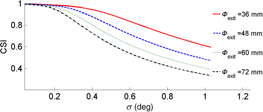

Table 1

Optimized starting point for CSI for different values of Φexit.

Φexit (mm)	36	48	60	72
Optimized ( $n_{0}, w_{0}$ ) (mm)	(5.6, 6.4)	(7.6, 8.2)	(9.2, 10.2)	(10.8, 12.2)
CSI ( $σ = 0.2 \deg$ ) (%)	98.309	97.749	96.709	94.847

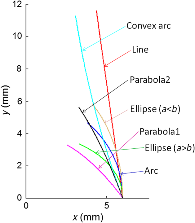
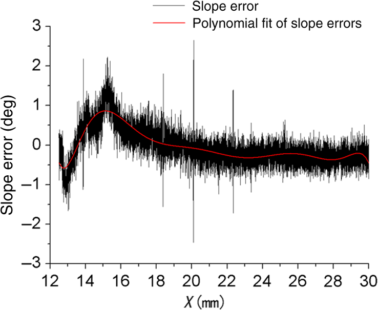
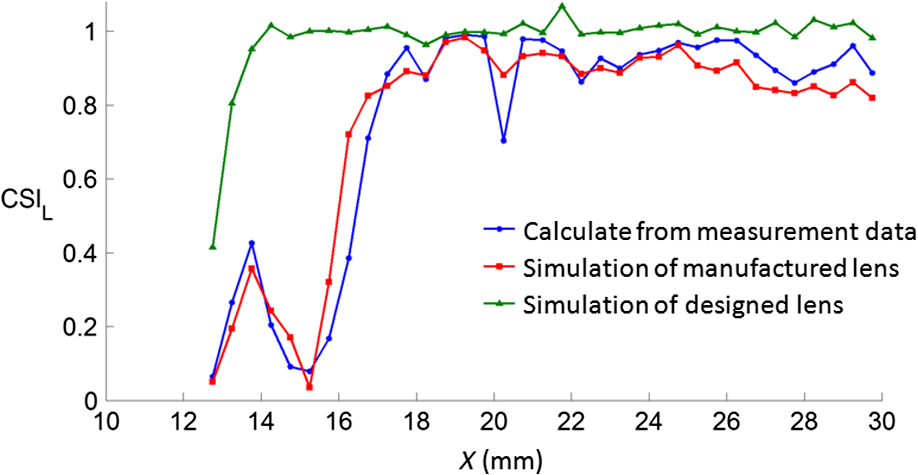
5.2.3.

Optimization of different types of inner curves

The tolerance characteristics of different types of the side incident surface are also discussed. The starting points of both the inner curve of the cross-section of the side incident surface and the TIR curve are the same, with $n_{0} = 6 mm$ and $w_{0} = 12 mm$ for all shapes. The shapes of the inner curves include an arc, a line, an elliptical curve with $a < b$ (where $a$ and $b$ are the semimajor and semiminor axes, respectively), an elliptical curve with $a > b$ , two parabolas, and a convex curve. The shapes of the inner curves are shown in Fig. 11, and the values of the slope error tolerances for each inner curve are plotted in Fig. 12. The results show that the tolerance of the TIR lens was poor at the base of the TIR surface, better in the middle, and slowly decreased toward the top. The convex inner curve has the best tolerance for the TIR surface, with the second best being the line. This means that there still might be space for us to optimize the design in light of tolerance considerations for inner curves other than a line.

Fig. 11

Shapes of different inner curves in the calculation. These include an arc, a line, an elliptic curve with $a < b$ , an elliptic curve with $a > b$ , two parabolas, and a convex curve.

Fig. 12

The tolerance of slope error with different types of inner curves. The convex inner curve has the best tolerance of the TIR surface, with the second best being the line.

6. Experiment and Discussion

One TIR lens with $Φ_{exit} = 60 mm$ and TIR surface designed with $n_{0} = 5.89 mm$ and $w_{0} = 12 mm$ was made, as in Fig. 13. Measurements proceed using an LED light source ZH-H095G from Foshan Evercore Optoelectronic Technology with a measured flux of 601 lm.²³ The diameter of the lighting emitting surface (LES) is 6 mm. The photometric data of the candela distribution are shown in Fig. 14. The full width at half maximum (FWHM) angle is 8.1 deg with a maximum luminous intensity of 15,140 cd.

Fig. 13

Lens with TIR surface designed with $n_{0} = 5.89 mm$ and $w_{0} = 12 mm$ . The contour was measured with the help of a contour graph (Taylor Hobsom Talysurf PGI Dimension 3). The accuracy of the measure of profilometry is 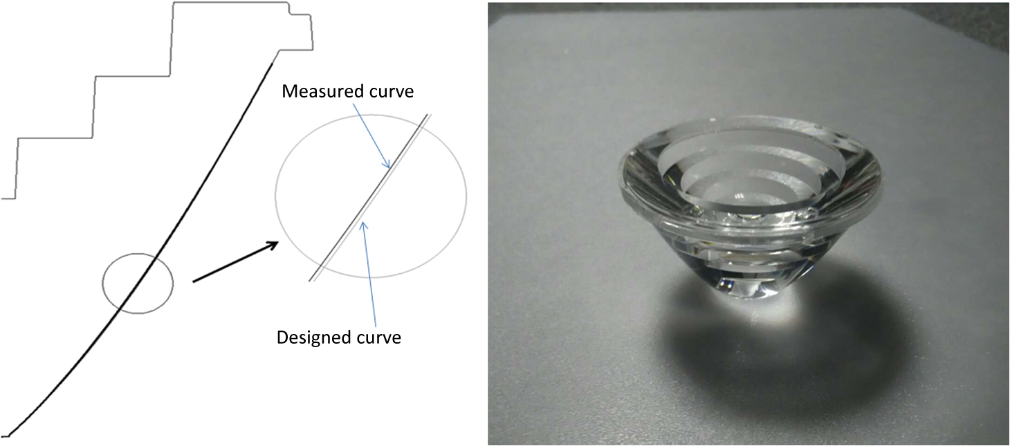$0.3 μ m / mm$ .

Fig. 14

The plot for measured candela distribution. The measuring flux of the LED light source is 601 lm and the diameter of LES is 6 mm.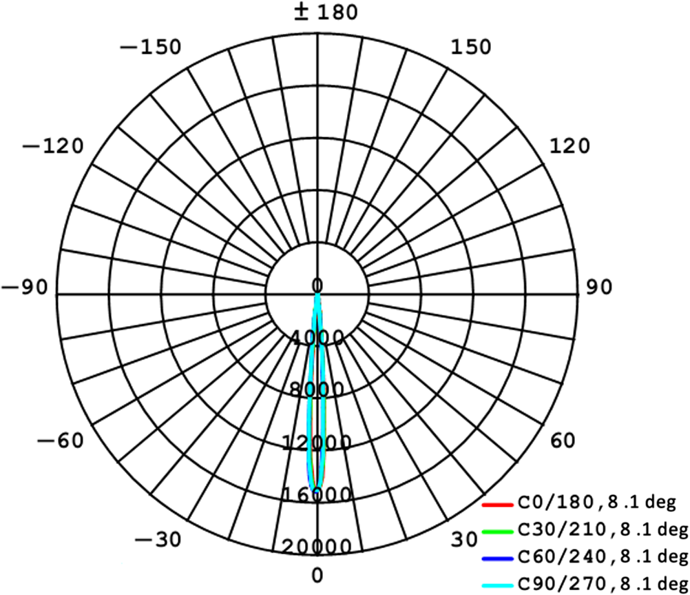

Figure 15 shows the one of the contours of the TIR surface measured by contour graph (Talysurf PGI Dimension 3 from Taylor Hobsom) and the designed model. The accuracy of the measure of profilometry is $0.3 μ m / mm$ . The fixed error $μ_{i}$ was secured by polynomial fitting as follows:

Eq. (11)

u (x) = B_{0} + B_{1} \cdot x + \dots + B_{9} \cdot x^{9} .

The index is shown in Table 2. The average value of

μ (x)

is 0.3388, and the standard deviation of the slope error

σ

varies from around 0.4 deg to about 0.2 deg, as in Fig. 16. We performed the CSI calculation using Eqs. (6)–(10) and compared the results in the simulation using Tracepro with 1 million rays, with the same luminary as that of Sec. 5 (i.e., a Lambertian disk with a radius of

R = 1 mm

). The simulation was made by dividing the TIR surfaces into different ring elements, each of which had the same size as the corresponding section in the contour measurement. When one of the elements was calculated, the other rings at the TIR surface were assumed to be absorbing to record the photometric data. The Fresnel loss characteristics of the optical surfaces were assumed in the simulation.

Fig. 15

The measured slope error and fitting of the TIR surface. A polynomial fitting was used.

Table 2

Fitted index of the fixed slope error.

B0	B1	B2	B3	B4	B5	B6	B7	B8	B9
71,416.8	$- 32, 545.27$	6509.59	$- 750.4$	54.967	$- 2.654$	0.0846	$- 0.00171$	$2.01 \times 10^{- 5}$	$- 1.03 \times 10^{- 7}$

Fig. 16

Standard deviation of the stochastic slope error measured from different parts of the TIR surface.

The comparison of ${CSI}_{L}$ between the calculated results and simulated results are shown in Fig. 17. We define RMS uniformity $D$ as follows:

Eq. (12)

D = \sqrt{\frac{\sum_{i = 1}^{n} {(y_{c} - y_{a})}^{2}}{\sum_{i = 1}^{n} y_{c}^{2}}},

where

y_{c}

is the calculated value and

y_{a}

is the simulated value received from simulating the measured contour. Using Eq. (12), we can calculate

D

to be 10.76%, which is quite small; in fact, the trend of the

{CSI}_{L}

is identical between the simulation and calculation, so the model of the slope-error tolerance’s impact on the CLI (based on CSI theory) described in this work reveals impressive agreement with the simulation results. Comparing measured results through photometry measurements to the designed

{CSI}_{L}

distribution can yield slope error information with the help of a CSI evaluation system.

Fig. 17

Comparison of ${CSI}_{L}$ with calculated results and simulated results from the measured contour data. The simulation was made by dividing the TIR surfaces into different ring elements, each of which has the same size as the corresponding section in the contour measurement.

7. Summary

TIR lenses as one LED collimators have been widely used and researched in the previous decades for the sake of performance optimization and compactness of design, despite the fact that scant research on manufacturing tolerances has been reported. This paper focused on the impact of manufacturing tolerance upon the CLI of the TIR surface and how to get better manufacturing tolerance through merit designs. First, the CSI was introduced as a metric for analyzing the performance of the CLI, both locally and as a whole, and the mechanism by which the CLI decreased was discussed; second, we introduced a unique design method to get better slope error tolerance; third, we optimized the initial parameters in the design to get a better CSI performance; finally, we fabricated a TIR lens by our design method and made a comparison between the tested contours of the TIR surfaces and the mathematical analysis and demonstrated the theoretical approach.

We are hopeful that this work can be sufficient to involve slope error analysis other than that of the meridian plane as well as the nonuniform distribution. Moreover, this work can be used further in the optimization of other types of collimating lenses, and that the impact of stochastic slope tolerance on the FWHM angle and utilization efficiency inside certain angles will be researched further with the help of the CSI evaluation method. Furthermore, nonuniform luminance and Fresnel losses should be considered to improve the theory and to expand its applications.

Acknowledgments

The authors thank the contour graph measurement from Guangzhou Institute of Measurement Detection and acknowledge support from the National Natural Science Foundation of China (Grant No. U1201254).

References

1.

T. Luo, C. Xu and G. Wang, “Concentration standard index (CSI) for ultra-compact LED collimated optical system evaluation,” in 2014 OSA Light, Energy and the Environment Congress, (2014). Google Scholar

2.

O. Dross and A. Eindhoven, “Investigation of the design space for low aspect ratio LED collimators,” Proc. SPIE, 8550 85502M (2012). http://dx.doi.org/10.1117/12.980512 PSISDG 0277-786X Google Scholar

3.

T. Kari et al., “Reliability of point source approximations in compact LED lens designs,” Opt. Express, 19 (S6), A1190 –A1195 (2011). http://dx.doi.org/10.1364/OE.19.0A1190 OPEXFF 1094-4087 Google Scholar

4.

D. Vázquez-Moliní et al., “High-efficiency light-emitting diode collimator,” Opt. Eng., 49 (12), 123001 (2010). http://dx.doi.org/10.1117/1.3522644 Google Scholar

5.

G. Z. Wang et al., “Collimating lens for light-emitting-diode light source based on non-imaging optics,” Appl. Opt., 51 (11), 1654 –1659 (2012). http://dx.doi.org/10.1364/AO.51.001654 APOPAI 0003-6935 Google Scholar

6.

X. T. Yan et al., “Design of a novel LED collimating element based on freeform surface,” Opt. Lett., 9 (1), 9 –12 (2013). http://dx.doi.org/10.1007/s11801-013-2331-0 OPLEDP 0146-9592 Google Scholar

7.

S. Zhao et al., “Lens design of LED searchlight of high brightness and distant spot,” J. Opt. Soc. Am. A, 28 (5), 815 –820 (2011). http://dx.doi.org/10.1364/JOSAA.28.000815 JOAOD6 0740-3232 Google Scholar

8.

G. Y. Yu et al., “A free-form total internal reflection (TIR) lens for illumination,” Proc. SPIE, 8321 832110 (2011). http://dx.doi.org/10.1117/12.903939 PSISDG 0277-786X Google Scholar

9.

Y. K. Zhen, Z. N. Jia and W. Z. Zhang, “The optimal design of TIR lens for improving LED illumination uniformity and efficiency,” Proc. SPIE, 6834 68342K (2007). http://dx.doi.org/10.1117/12.756101 PSISDG 0277-786X Google Scholar

10.

X. X. Meng et al., “Design of LED collimator for uniform illumination with double freeform surfaces,” Acta Photon. Sin., 43 (8), 082200 (2014). http://dx.doi.org/10.3788/gzxb20144308.0822003 Google Scholar

11.

C. R. Prins et al., “An inverse method for the design of TIR collimators to achieve a uniform color light beam,” J. Eng. Math., 81 177 –190 (2013). http://dx.doi.org/10.1007/s10665-012-9584-7 JLEMAU 0022-0833 Google Scholar

12.

R. S. Chen, “Investigation of a slope-point-based method for the design of aspheric surfaces in a catadioptric collimating optical system for a light-emitting diode source,” Appl. Opt., 53 (29), H129 –H139 (2014). http://dx.doi.org/10.1364/AO.53.00H129 APOPAI 0003-6935 Google Scholar

13.

W. A. Parkyn, “The design of illumination lenses via extrinsic differential geometry,” Proc. SPIE, 3428 154 –162 (1998). http://dx.doi.org/10.1117/12.327958 PSISDG 0277-786X Google Scholar

14.

Y. N. Shen, Y. F. Huang and X. Han, “Design of collimating system for LED source,” Proc. SPIE, 9042 90420V (2013). http://dx.doi.org/10.1117/12.2034984 PSISDG 0277-786X Google Scholar

15.

J. J. Chen and C. T. Lin, “Freeform surface design for a light-emitting diode-based collimating lens,” Opt. Eng., 49 (9), 093001 (2010). http://dx.doi.org/10.1117/1.3488046 Google Scholar

16.

J. J. Chen et al., “Freeform lens design for LED collimating illumination,” Opt. Express, 20 (10), 10984 –10995 (2012). http://dx.doi.org/10.1364/OE.20.010984 OPEXFF 1094-4087 Google Scholar

17.

M. González-Montes et al., “Optics detailed analysis of an improved collimation system for LED light sources,” Proc. SPIE, 8170 81700F (2011). http://dx.doi.org/10.1117/12.896795 PSISDG 0277-786X Google Scholar

18.

W. D. Huang and Z. F. Han, “Theoretical analysis of error transfer from the surface slope to the reflected ray and their application in the solar concentrated collector,” Sol. Energy, 86 2592 –2599 (2012). http://dx.doi.org/10.1016/j.solener.2012.05.029 Google Scholar

19.

Nonimaging Optics, 395 –413 Elsevier(2005). Google Scholar

20.

W. D. Huang, Y. P. Li and Z. F. Han, “Theoretical analysis of error transfer from surface slope to refractive ray and their application to the solar concentrated collector,” Renew. Energy, 57 562 –569 (2013). http://dx.doi.org/10.1016/j.renene.2013.02.029 RNENE3 0960-1481 Google Scholar

21.

F. Z. Fang et al., “Manufacturing and measurement of freeform optics,” CIRP Ann. Manuf. Technol., 62 823 –846 (2013). http://dx.doi.org/10.1016/j.cirp.2013.05.003 Google Scholar

22.

D. Y. Yu and H. Y. Tan, Engineering Optics, Chinese Machinery Industry Press, Beijing, China (2011). Google Scholar

23.

Product data sheet of ZH-H095G is in the catalog of Commercial Lighting of LED COB products, (2015) http://www.evercore.cn/en/pro1.asp January ). 2015). Google Scholar

Biography

Tao Luo received his bachelor’s degree from the electronic engineering department of Tianjin University in 2004 and his master’s degree from the electronic engineering department of Tsinghua University in 2007. He has worked in the field of LED optical design for more than eight years. He is currently attending doctorate courses at Sun Yat-sen University in optical engineering under the supervision of Prof. Gang Wang.

Gang Wang is a professor at the School of Electronics and Information Engineering, Sun Yat-sen University, and also dean of Foshan Institute of Sun Yat-sen University. He received his PhD in 2001 from Nagoya Institute of Technology in Japan, and was employed by the State Key Laboratory of Optoelectronic Materials Technologies of Sun Yat-sen University in 2004. He is developing wide band-gap semiconductor and LED lighting. He has published more than 50 patents in these fields.

CC BY: © The Authors. Published by SPIE under a Creative Commons Attribution 4.0 Unported License. Distribution or reproduction of this work in whole or in part requires full attribution of the original publication, including its DOI.

Citation Download Citation

Tao Luo and Gang Wang "Design and optimization for total internal reflection collimators based on slope-error tolerance analysis," Optical Engineering 55(2), 025103 (2 February 2016). https://doi.org/10.1117/1.OE.55.2.025103

Published: 2 February 2016

Access the abstract

JOURNAL ARTICLE
8 PAGES

DOWNLOAD PAPER SAVE TO MY LIBRARY

GET CITATION

CITATIONS

Cited by 5 scholarly publications.

Explore citations on Lens.org

KEYWORDS

Tolerancing

Light emitting diodes

Collimators

Light sources

Reflection

Lenses

Error analysis

1.

Introduction

2.

Slope Error Problems in Total Internal Reflection Lenses

2.1.

Total Internal Reflection Lenses Structure

Fig. 1

2.2.

Analysis Model of Total Internal Reflection Lenses

2.3.

Central Luminous Intensity Decrease Mechanics

Fig. 2

2.4.

Concentration Standard Index

Eq. (1)

Eq. (2)

Eq. (3)

Eq. (4)

Eq. (5)

3.

Concentration Standard Index Calculations of Total Internal Reflection Lenses

Eq. (6)

Eq. (7)

Eq. (8)

Eq. (9)

4.

Total Internal Reflection Design for Improved Manufacturing Tolerance

Fig. 3

5.

Results and Discussion

Eq. (10)

5.1.

Slope-Error Tolerance of the Total Internal Reflection Surface

Fig. 4

Fig. 5

5.2.

Optimization for Better Slope-Error Tolerance

5.2.1.

Optimization of the total internal reflection curve with a conical inner surface

Fig. 6

Fig. 7

Fig. 8

Fig. 9

5.2.2.

Comparison of concentration standard index with different sizes of total internal reflection lenses

Fig. 10

Table 1

5.2.3.

Optimization of different types of inner curves

Fig. 11

Fig. 12

6.

Experiment and Discussion

Fig. 13

Fig. 14

Eq. (11)

Fig. 15

Table 2

Fig. 16

Eq. (12)

Fig. 17

7.

Summary

Acknowledgments

References

Biography

Show All Keywords

Keywords/Phrases

Search In:

Publication Years