Maximum likelihood estimation of vehicle position for outdoor image sensor-based visible light positioning system

Xiang Zhao; Jiming Lin

doi:10.1117/1.OE.55.4.043104

18 April 2016 Maximum likelihood estimation of vehicle position for outdoor image sensor-based visible light positioning system

Xiang Zhao, Jiming Lin

Author Affiliations +

Optical Engineering, Vol. 55, Issue 4, 043104 (April 2016). https://doi.org/10.1117/1.OE.55.4.043104

Abstract

Image sensor-based visible light positioning can be applied not only to indoor environments but also to outdoor environments. To determine the performance bounds of the positioning accuracy from the view of statistical optimization for an outdoor image sensor-based visible light positioning system, we analyze and derive the maximum likelihood estimation and corresponding Cramér–Rao lower bounds of vehicle position, under the condition that the observation values of the light-emitting diode (LED) imaging points are affected by white Gaussian noise. For typical parameters of an LED traffic light and in-vehicle camera image sensor, simulation results show that accurate estimates are available, with positioning error generally less than 0.1 m at a communication distance of 30 m between the LED array transmitter and the camera receiver. With the communication distance being constant, the positioning accuracy depends on the number of LEDs used, the focal length of the lens, the pixel size, and the frame rate of the camera receiver.

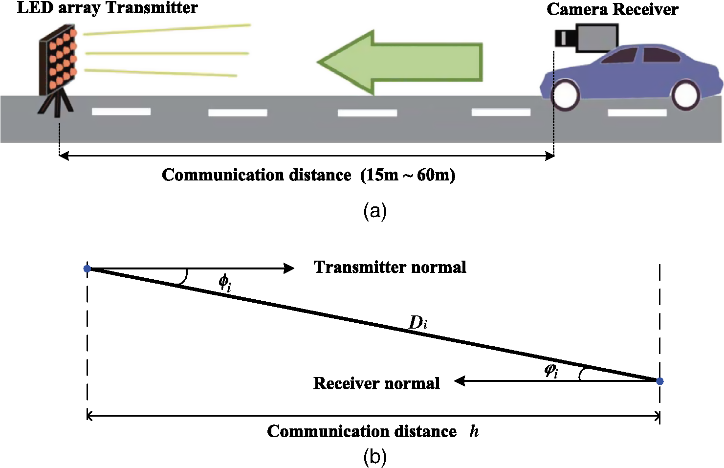
1. Introduction

In recent years, with the rapid development of solid-state lighting technology, white light-emitting diodes (LEDs) have been widely used in the field of lighting, displaying, and transmitting and/or receiving of data.¹^,² Compared with incandescent and fluorescent lights, white LEDs have the characteristic of long life expectancy, high energy efficiency, and low cost, and they can be modulated at a relatively high speed that is undetectable to the human eye. To date, a considerable amount of white LED–based research has been developed and may fall into two categories: visible light communication (VLC) and visible light positioning (VLP).

For VLC, the intrinsic features of white LEDs makes them suitable for high speed communication. First, VLC is based on the lighting function of white LEDs. To ensure sufficient light intensity, 400 to 1000 lux³ is often required for illumination levels. Therefore, the signal-to-noise ratio is high enough for VLC. Second, the radiation spectrum of white LEDs spans from 400 to 800 THz; thus high channel capacity could be achievable in accordance with the Shannon formula. At present, most researches on high speed VLC are confined to the indoor environment, mainly to improve the modulation bandwidth of LEDs,⁴ develop improved modulation technology,⁵ and design multiplexing scheme.⁶ The highest data rate reported so far is the wave division multiplexing (WDM) VLC system,⁷ where carrierless amplitude and phase modulation technology and adaptive equalization technology are jointly used to achieve a data rate of 4.5 Gbps in the laboratory.

For VLP,⁸^–¹⁰ according to the optical reception devices used at the receiver, it can be divided into the photodiode (PD)-based VLP and the image sensor (IS)-based VLP. Since the PD is susceptible to the direction of the light beam, if it is flipped over or moved out of the range covered by the LED, the PD-based VLP system could fail; thus it has limited mobility and is only suitable for slow speed motion or quasistatic condition. In addition, PDs cannot be utilized in outdoor direct solar radiation environment. This is because PDs can only detect the optical power of incoming light; because direct solar radiation is usually strong, the PD is saturated by the intense optical power since it has a limited response. Therefore, most of the PD-based VLPs proposed belong to indoor positioning.¹¹^–¹⁷

For the IS-based VLP,⁹^,¹⁸^–²⁰ IS is used as an optical reception device. IS can detect not only the intensity but also the angle of arrival (AOA) of incoming light. IS consists of many pixels, and different light sources can be spatially separated using their imaging points on IS. Here, the light sources include various LED sources (such as indoor LED dome light, outdoor LED traffic light, LED brake light, or headlight of a vehicle) and noise sources (such as the Sun and other ambient lights). Via differentiating the imaging positions of light sources, LED sources can be recognized by a simple feature matching algorithm from multiple noise sources. Consequently, the IS-based VLP is available not only for indoor but also outdoor environments. Furthermore, combined with image processing and digital signal processing technology, the IS-based VLP can be utilized for safety driving such as collision warning and avoidance, lane change assistance, pedestrian detection, and adaptive cruise control.

To date, the published papers on the IS-based VLP have mostly focused on the field of applied research, such as indoor navigation systems,²¹ outdoor intelligent traffic systems,²²^–²⁵ and various location-based services.²⁶ These researches have shown that accurate localization can be achievable; however, little has been published about the analytical performance bounds of the positioning accuracy from the view of statistical optimization. The determination of the positioning accuracy will allow the optimization of the parameters governing the IS-based VLP systems.

The contributions of this paper are as follows. First, we analyze and derive the maximum likelihood estimation (MLE) and corresponding Cramér–Rao lower bounds (CRLB) for a typical outdoor IS-based VLP system, assuming white Gaussian model for system noise. Second, we analyze the effect of system parameters on CRLB. When a camera IS is used as receiver, there exist several types of noise generated from IS. As shot noise takes the dominant role, the system noise variance is influenced by many factors, such as the total received optical power, the pixel size, the focal length, and the frame rate of the camera receiver. Because the derived CRLB is proportional to system noise variance, we will emphatically analyze the system noise and the parameters affecting system noise variance in this paper.

The rest of this paper is organized as follows. In Sec. 2, an outdoor IS-based VLP system model is introduced, where the transmitter is the LED array of traffic light, and the camera receiver is assumed to be mounted on the dashboard of a vehicle. In Sec. 3, the MLE of the vehicle position is derived under the condition that the observation values of the LEDs’ imaging points are affected by white Gaussian noise. The performance analysis is completed in Sec. 4, where the CRLB is deduced and the parameters affecting CRLB are analyzed in detail. In Sec. 5, simulation results are given for a typical outdoor scenario. Conclusions are made in Sec. 6.

Notations: The operators ${\cdot}^{T}$ , $E [\cdot]$ , and $var (\cdot)$ denote the transpose of a matrix, the expectation, and the variance of a random variable or matrix, respectively.

2. System Model

For the outdoor IS-based VLP system, as shown in Fig. 1, the transmitter may be the LED array of the traffic light in a city crossing, and the receiver may be a camera IS mounted on the dashboard of a vehicle. The signal from the LED and the image of the LED on the camera receiver are jointly used to determine the location of the receiver, which is assumed to be the vehicle position.

Fig. 1

An outdoor IS-based VLP system model, where any LED $P_{i}$ from the LED array transmitter is imaged through the pinhole $O_{s}$ onto an imaging point $p_{i}$ in the image plane of the camera receiver fixed on a vehicle, with $P_{i} = {(X_{i}, Y_{i}, Z_{i})}^{T}$ , $i = 1, 2, \dots, N$ being the 3-D world coordinate; $p_{i} = {(x_{i}, y_{i})}^{T}$ , $i = 1, 2, \dots, N$ being the 2-D image plane coordinate; and $O_{s} = {(X_{s}, Y_{s}, Z_{s})}^{T}$ being the 3-D world coordinate of the center of the camera receiver. The goal is to estimate the vehicle position, which is assumed to be the world coordinates $O_{s}$ of the center of the camera receiver under the condition that the system is affected by white Gaussian noise. The system parameters are listed in Table 1.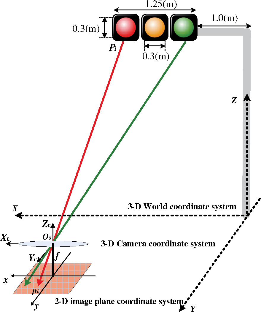

Table 1

System parameters.

Parameter	Value
Height of traffic light	$Z_{i} = 6.21$ (m)
Height of camera receiver	$Z_{s} = 1.0$ (m)
Length of traffic arm	1.0 (m)
Width of lane	3.5 (m)
Width of vehicle	1.8 (m)

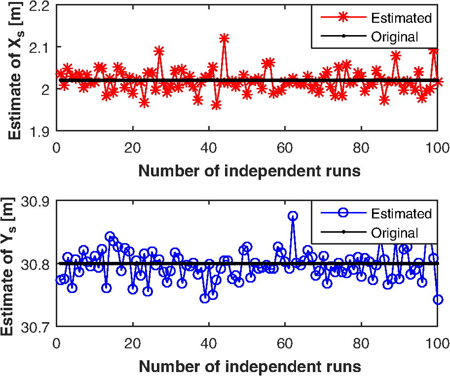
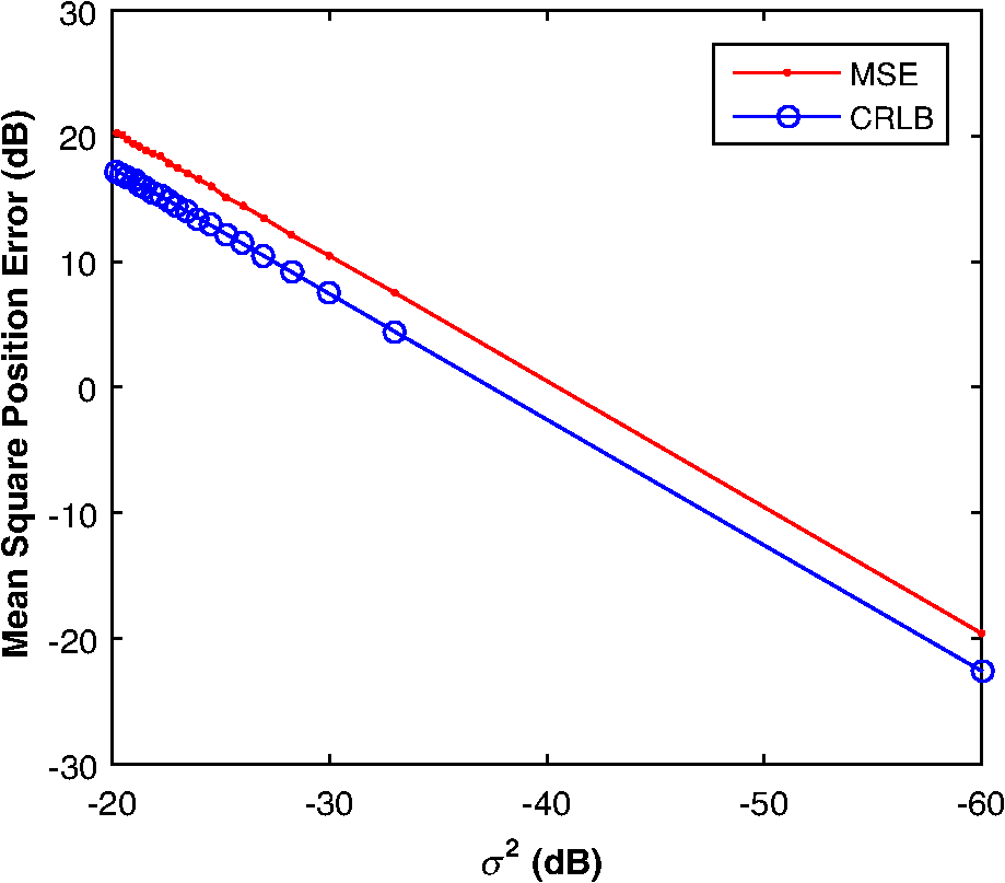
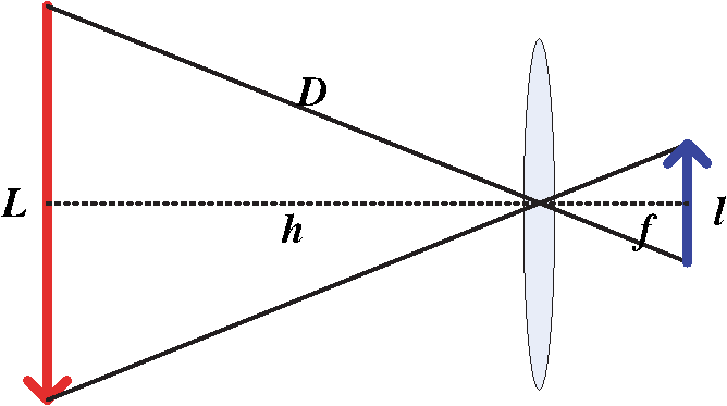
In Fig. 1, there are three coordinate systems, which are the three-dimensional (3-D) world coordinate system, the 3-D camera coordinate system, and the two-dimensional (2-D) image plane coordinate system. Any LED $P_{i}$ ( $i = 1, 2, \dots, N$ ) from the LED array transmitter is imaged into an imaging point $p_{i}$ ( $i = 1, 2, \dots, N$ ) in the image plane through the center of the lens. It is assumed that LED $P_{i}$ ( $i = 1, 2, \dots, N$ ) is located at $P_{i} = {(X_{i}, Y_{i}, Z_{i})}^{T}$ in the 3-D world coordinate system and is known a priori. The imaging point of LED $P_{i}$ is $p_{i} = {(x_{i}, y_{i})}^{T}$ ( $i = 1, 2, \dots, N$ ) in the 2-D image plane coordinate system, which can be measured via image processing and signal processing technologies. However, the measurement value of the imaging point is often influenced by noise. When shot noise is the dominant noise source, system noise can be viewed as white Gaussian noise.²⁷^,²⁸ Hence, our goal is to estimate the location of the camera receiver for white Gaussian noise, to obtain the MLE, and finally derive the CRLB.

For any LED $P_{i}$ from the LED array transmitter, it satisfies

Eq. (1)

P_{i} = R P_{c i} + O_{s},

where

P_{c i} = {(X_{c i}, Y_{c i}, Z_{c i})}^{T}

,

i = 1, 2, \dots, N

is the coordinate of LED

P_{i}

in the camera coordinate system. The camera coordinate system is such a system where its origin is located at the center of the camera receiver, the direction of

Z_{c}

is perpendicular to the 2-D image plane, and the

Z_{c}

axis is usually called the optical axis.

R

is the rotation matrix of the camera receiver from the camera coordinate system to the world coordinate system, which is a

3 \times 3

orthogonal matrix.

O_{s} = {(X_{s}, Y_{s}, Z_{s})}^{T}

is the world coordinate of the center of the camera receiver, which is assumed to be the vehicle position since the camera receiver is fixed on a vehicle, supposably on the dashboard of a vehicle.

The rotating process of the camera receiver from the camera coordinate system to the world coordinate system is shown in Fig. 2. The rotation angle $ϕ$ and $ω$ can be directly read out from the inclination sensor attached in the camera receiver; however, the azimuth angle $κ$ has to be calculated:

Eq. (2)

R = (\begin{matrix} r_{11} & r_{12} & r_{13} \\ r_{21} & r_{22} & r_{23} \\ r_{31} & r_{32} & r_{33} \end{matrix}) = (\begin{matrix} \cos ϕ & 0 & - \sin ϕ \\ 0 & 1 & 0 \\ \sin ϕ & 0 & \cos ϕ \end{matrix}) (\begin{matrix} 1 & 0 & 0 \\ 0 & \cos ω & - \sin ω \\ 0 & \sin ω & \cos ω \end{matrix}) (\begin{matrix} \cos κ & - \sin κ & 0 \\ \sin κ & \cos κ & 0 \\ 0 & 0 & 1 \end{matrix}) .

For simplicity in this paper we assume that the vehicle is running on a reasonably flat terrain plane without azimuth rotation; that is to say, the orientation of the camera coordinate system is the same as that of the world coordinate system so that the rotation matrix from the camera coordinate system to the world coordinate system can be expressed as

R = E

, where

E

denotes an identity matrix. In addition, since the camera receiver is fixed on the dashboard of a vehicle, the height

Z_{s}

of the camera receiver is known a priori, then the distance (between the traffic light and camera receiver) along the direction of the optical axis is

h = Z_{i} - Z_{s}

.

Fig. 2

Rotating process of the camera receiver from the camera coordinate system to the world coordinate system.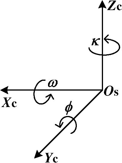

In the 3-D camera coordinate system, the relationship between $P_{c i} = {(X_{c i}, Y_{c i}, Z_{c i})}^{T}$ , $i = 1, 2, \dots, N$ and $p_{i} = {(x_{i}, y_{i})}^{T}$ , $i = 1, 2, \dots, N$ can be described, with the focal length of the lens being $f$ , as

Eq. (3)

\frac{X_{c i}}{x_{i}} = \frac{Y_{c i}}{y_{i}} = \frac{Z_{c i}}{- f} .

Rearranging Eqs. (1) and (3), we get the mathematical relationship between the LEDs

{(X_{i}, Y_{i})}_{i = 1}^{N}

and the measurement values

{({\tilde{x}}_{i}, {\tilde{y}}_{i})}_{i = 1}^{N}

of their imaging points, which can be written as

Eq. (4)

(\begin{matrix} {\tilde{x}}_{i} \\ {\tilde{y}}_{i} \end{matrix}) = (- \frac{f}{h}) (\begin{matrix} X_{i} - X_{s} \\ Y_{i} - Y_{s} \end{matrix}) + (\begin{matrix} n_{x i} \\ n_{y i} \end{matrix}),

where the measurement noise

{n_{x i}}_{i = 1}^{N}

and

{n_{y i}}_{i = 1}^{N}

are independently white Gaussian noise of the direction

x

and

y

in the 2-D IS plane, with the same mean 0 and variance

σ^{2}

.

Our goal is to estimate the parameter vector $r = {(X_{s}, Y_{s})}^{T}$ of the vehicle position, derive its MLE, and finally get the CRLB for white Gaussian noise.

3. Maximum Likelihood Estimation

Based on the measurement values ${{\tilde{x}}_{i}}_{i = 1}^{N}$ and ${{\tilde{y}}_{i}}_{i = 1}^{N}$ and the LED coordinates ${X_{i}}_{i = 1}^{N}$ and ${X_{i}}_{i = 1}^{N}$ , the log-likelihood function of the parameter vector $r = {(X_{s}, Y_{s})}^{T}$ of the vehicle position is given as

Eq. (5)

\ln (X_{s}, Y_{s}, σ^{2}) = (- \frac{N}{2}) \ln (2 π σ^{2}) - \frac{1}{2 σ^{2}} \sum_{i = 1}^{N} [{((\frac{f}{h}) [X_{i} - X_{s}] + {\tilde{x}}_{i})}^{2} + {((\frac{f}{h}) [Y_{i} - Y_{s}] + {\tilde{y}}_{i})}^{2}] .

Differentiating the log-likelihood function with respect to

X_{s}

gives

Eq. (6)

\frac{\partial \ln (X_{s}, Y_{s})}{\partial X_{s}} = \frac{f}{σ^{2} h} \sum_{i = 1}^{N} [(\frac{f}{h}) [X_{i} - X_{s}] + {\tilde{x}}_{i}] .

Let

\partial \ln (X_{s}, Y_{s}) / \partial X_{s} = 0

; then the MLE of the position parameter

X_{s}

is given as

Eq. (7)

{\hat{X}}_{s} = \frac{1}{N} \sum_{i = 1}^{N} X_{i} + \frac{h}{N f} \sum_{i = 1}^{N} {\tilde{x}}_{i} .

Similarly, differentiating the log-likelihood function with respect to $Y_{s}$ gives

Eq. (8)

\frac{\partial \ln (X_{s}, Y_{s})}{\partial Y_{s}} = \frac{f}{σ^{2} h} \sum_{i = 1}^{N} [(\frac{f}{h}) [Y_{i} - Y_{s}] + {\tilde{y}}_{i}] .

Let

\partial \ln (X_{s}, Y_{s}) / \partial Y_{s} = 0

; then the MLE of the position parameter

Y_{s}

is given as

Eq. (9)

{\hat{Y}}_{s} = \frac{1}{N} \sum_{i = 1}^{N} Y_{i} + \frac{h}{N f} \sum_{i = 1}^{N} {\tilde{y}}_{i} .

Define $\frac{1}{N} \sum_{i = 1}^{N} X_{i} = {\bar{X}}_{i}, \frac{1}{N} \sum_{i = 1}^{N} Y_{i} = {\bar{Y}}_{i}, \frac{1}{N} \sum_{i = 1}^{N} {\tilde{x}}_{i} = \bar{x}, \frac{1}{N} \sum_{i = 1}^{N} {\tilde{y}}_{i} = \bar{y}$ .

We can express the MLE of the vehicle position as

Eq. (10)

{\begin{cases} {\hat{X}}_{s} = \bar{X} + \frac{h}{f} \bar{x} \\ {\hat{Y}}_{s} = \bar{Y} + \frac{h}{f} \bar{y} \end{cases} .

Consequently, the MLE of the vehicle position can be obtained by finding the means of measurement values ${{\tilde{x}}_{i}}_{i = 1}^{N}$ and ${{\tilde{y}}_{i}}_{i = 1}^{N}$ , and the means of LEDs coordinates ${X_{i}}_{i = 1}^{N}$ and ${X_{i}}_{i = 1}^{N}$ .

Figure 3 shows the estimation values of $X_{s}$ and $Y_{s}$ when $σ$ is $10^{- 3}$ . It can be seen that the estimation values vibrate around the original value ( $X_{s} = 2.02 m$ and $Y_{s} = 30.8 m$ ), and this is because the program is run independently each time.

Fig. 3

Estimation of $X_{s}$ and $Y_{s}$ when $σ = 10^{- 3}$ .

4. Performance Analysis

The CRLB gives a lower bound on variance attainable by any unbiased estimation. In order to better illustrate the performance of an estimation method, it can be compared with the CRLB. The regularity condition of the CRLB²⁹ holds for the given estimation since Eqs. (6) and (8) are finite, and the expected value of Eqs. (6) and (8) is 0.

The CRLB of the vector parameter $r = {(X_{s}, Y_{s})}^{T}$ can be obtained through three steps. First, from Eqs. (6) and (8) we get the second-order derivatives of the log-likelihood function with respect to $X_{s}$ and $Y_{s}$ , respectively. Second, taking the negative expectations of the second-order derivatives yields

Eq. (11)

{\begin{cases} - E [\frac{\partial^{2} \ln (X_{s}, Y_{s})}{\partial X_{s}^{2}}] = \frac{N f^{2}}{h^{2} σ^{2}} \\ - E [\frac{\partial^{2} \ln (X_{s}, Y_{s})}{\partial Y_{s}^{2}}] = \frac{N f^{2}}{h^{2} σ^{2}} \\ - E [\frac{\partial^{2} \ln (X_{s}, Y_{s})}{\partial X_{s} \partial Y_{s}}] = 0 \end{cases} .

The $2 \times 2$ Fisher information matrix $I (r)$ is written as

Eq. (12)

I (r) = (\begin{matrix} - E [\frac{\partial^{2} \ln (X_{s}, Y_{s})}{\partial X_{s}^{2}}] & - E [\frac{\partial^{2} \ln (X_{s}, Y_{s})}{\partial X_{s} \partial Y_{s}}] \\ - E [\frac{\partial^{2} \ln (X_{s}, Y_{s})}{\partial Y_{s} \partial X_{s}}] & - E [\frac{\partial^{2} \ln (X_{s}, Y_{s})}{\partial Y_{s}^{2}}] \end{matrix}) .

Finally, the CRLB of the vector parameter

r = {(X_{s}, Y_{s})}^{T}

can be derived by taking the

[i, i]

’th element of the inverse of

I (r)

, namely,

i = 1,2

, from Ref. 29. The inverse of the

2 \times 2

Fisher information matrix

r = {(X_{s}, Y_{s})}^{T}

is expressed as

Eq. (13)

I^{- 1} (r) = (\begin{matrix} \frac{h^{2} σ^{2}}{N f^{2}} & 0 \\ 0 & \frac{h^{2} σ^{2}}{N f^{2}} \end{matrix}) .

Consequently, the CRLB of the vehicle position for white Gaussian noise is given as

Eq. (14)

{\begin{cases} var ({\hat{X}}_{s}) \geq \frac{h^{2} σ^{2}}{N f^{2}} \\ var ({\hat{Y}}_{s}) \geq \frac{h^{2} σ^{2}}{N f^{2}} \end{cases} .

Figure 4 shows the performance comparison of CRLB and mean square positioning error (MSPE) at

σ^{2} \in [- 20,60] dB

. MSPE is defined as

E [{({\hat{X}}_{s} - X_{s})}^{2} + {({\hat{Y}}_{s} - Y_{s})}^{2}]

. Note that the decibel scale is employed in both axes in order to facilitate the presentation.³⁰ It can be seen that the MSPE is proportional to

σ^{2}

and is unlimitedly close to the CRLB.

Fig. 4

Comparison of CRLB and MSPE.

From Eq. (14), we know that the CRLB is proportional to the noise variance $σ^{2}$ , with the number of LEDs used $N$ , the focal length of the camera receiver $f$ , and the distance $h$ being known. However, when a camera IS is used as receiver for an outdoor IS-based VLP system, there exist several types of noise generated from IS. When shot noise takes the dominant role, the system noise variance is influenced by many factors, such as the total received optical power, the pixel size, the focal length, and the frame rate of camera receiver.

In the following, we will emphatically analyze the system noise in the IS-based VLP system and the parameters affecting system noise variance.

4.1.

System Noise

There are two basic types of noise generated by IS, which are pattern noise (PN) and random noise (RN). PN can be directly observed by human eyes and distributed in a spatial form, which does not vary with each frame of image. The effect of PN on image quality is far greater than RN, but it can be effectively inhibited or eliminated through the correlated double sampling or flat field correction technology. Hence, the effect of PN will not be considered in this paper.

The quantized values of RN vary with each frame of image, and RN obeys a statistical distribution. One typical RN is shot noise, and it is generated by random variation of photoinduced charge carriers with incoming light in the semiconductor of the camera receiver. When the number of photoinduced charge carriers is large enough, shot noise is in Gaussian distribution and is white noise. In the IS-based VLP system, shot noise is mainly made up of three parts: quantum noise generated from the observation point of the image corresponding to each LED, quantum noise coming from the interference of other LEDs, ambient light noise from fluorescent or incandescent lights or the sun, and so on. Since IS has the ability to spatially separate sources, the imaging points of discrete LEDs on the camera IS receiver can be resolved; that is, noise from the interference of other LEDs is so small that it can be classified into ambient light noise. Hence, while shot noise takes the dominant role, the system noise variance can be expressed as

Eq. (15)

σ^{2} = σ_{shot}^{2} = 2 q ρ (P_{r} + P_{n} A_{total}) \cdot I_{2} R_{b},

where

q

is the electronic charge,

ρ

is the conversion coefficient from the optical to electrical domain and is often assumed to be that

0.4 mA / mW

,

P_{r}

is the total received optical power of the camera receiver,

P_{n}

is the power of ambient light noise on unit area,

A_{total}

is the total detecting area of IS,

A

is the effective detecting area corresponding to a single LED,

I_{2}

is the noise bandwidth factor, and often,

I_{2} = 0.562

, and

R_{b}

is the data transmission rate. Because the frame rate is equal to the sampling rate of the camera, if Nyquist sampling is used, the frame rate of the camera should be at least twice the data transmission rate.

4.2.

Parameters Affecting System Noise Variance

In this paper, such a channel scenario is utilized for the outdoor IS-based VLP system, as shown in Fig. 5(a), where the LED array transmitter is placed on horizontal ground and the camera receiver is fixed on the dashboard of a vehicle, with the center of the LED array transmitter in the optical axis of the camera receiver.

Fig. 5

Transmitter–receiver channel: (a) experimental scenario and (b) lateral view.

4.2.1.

Total received optical power

If $N$ LEDs are used to locate an IS receiver, the total received optical power $P_{r}$ of IS is $P_{r} = \sum_{i = 1}^{N} H_{i} (0) P_{t}$ , when each LED transmits constant optical power $P_{t}$ for each line of sight (LOS) channel. A lateral view of the transmitter–receiver channel is shown in Fig. 5(b). For the $i$ ’th channel, $i = 1,2, \dots, N$ , $H_{i} (0) = \frac{(m + 1) \cos^{m} (ϕ_{i}) \cos (φ_{i}) A}{2 π D_{i}^{2}}$ is the directed circuit gain, $m$ is the order of Lambertian emission and generally $m = 1$ , $ϕ_{i}$ is angle of irradiance, $φ_{i}$ is the angle of incidence with $0 \leq φ_{i} \leq φ_{C}$ , and $φ_{C}$ is the field of view (FOV) of the IS receiver. $D_{i}$ is the propagation distance from each LED transmitter to the camera receiver. For the communication distance between the LED transmitter and camera receiver being $h$ , if $ϕ_{i} = φ_{i}$ then $\cos (ϕ_{i}) = h / D_{i}$ , and the total received optical power can be expressed as

Eq. (16)

P_{r} = C (φ) \cdot P_{t} \cdot h^{- 2} \cdot A,

where

C (φ) = \sum_{i = 1}^{N} [(m + 1) \cos^{m + 3} (φ_{i}) / 2 π]

, which is related to incidence angles. It is assumed that all incidence angles of LOS links are within the FOV of the receiver.

4.2.2.

Effective area for detecting

It is necessary to calculate the image size corresponding to one LED when a camera IS is used for receiver. The imaging process of a single LED through the lens on the camera IS is shown in Fig. 6. According to Newton’s formula, if the diameters of the LED and the corresponding image are $L$ and $l$ , respectively, for a focal length of $f$ and a distance of $h$ between the LED and the lens, then the relationship between these parameters satisfies $l = f L / h$ . It is referred to the distance where the LED generates an image that falls into exactly one pixel as the critical distance $d_{c}$ . If $h \geq d_{c}$ , the image of the LED falls into only one pixel; then the effective area for detecting is $A = w^{2}$ , where $w$ is the width of a pixel. If $h < d_{c}$ , the image of LED will fall into several pixels; then $A = l^{2} = {(f L / h)}^{2}$ .

Fig. 6

Imaging process of a single LED on the camera IS.

5. Numerical Results

Simulation experiments are performed in a channel scenario, as shown in Fig. 5(a), where the LED array transmitter is placed on horizontal ground and the camera receiver is fixed on the dashboard of a vehicle, with the center of the LED array transmitter in the optical axis of the camera receiver. The communication distance between the LED array transmitter and the camera receiver is changed from 15 to 60 m, every 5 m on a static condition. The white LEDs are used for the LED array transmitter, and a Photron IDP-Express R2000 is used for the camera IS receiver. The parameters are listed in Tables 2 and 3, respectively.

Table 2

Parameters for the LED array transmitter.

Parameter	Value
Number of LEDs	$32 \times 32$
Spacing of LEDs	15 (mm)
Size of LED array	$465 mm \times 465 mm$
Diameter of an LED	$L = 6$ (mm)
Transmitted optical power of an LED	$P_{t} = 100$ (mW)

Table 3

Parameters for the camera image sensor receiver.

Parameter	Value
Focal length	$f = 35$ (mm)
Pixel size	$w = 10$ ( $μ m$ )
Frame rate	$R_{s} = 1000$ (fps)
Resolution	$1024 pixel \times 1024 pixel$

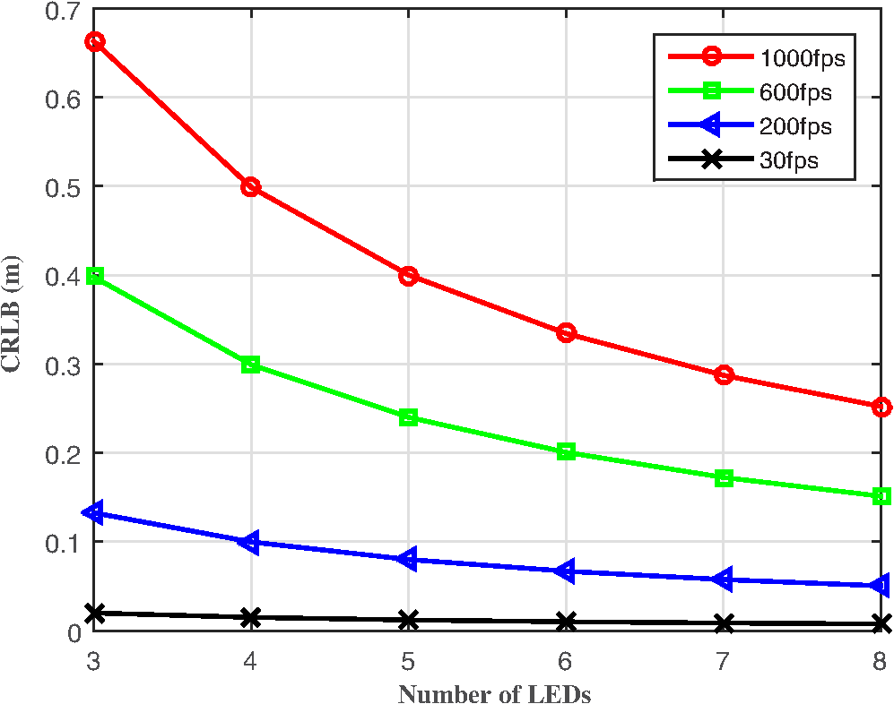
In the following, we will present simulation results for the CRLB for the positioning system described in the previous section for a range of parameters, such as the communication distance, the pixel size, and the focal length and frame rate of the camera receiver.

First, we study the influence of the communication distance on CRLB. Figure 7 shows the CRLB versus the communication distance between the LED transmitter and camera receiver, from 15 to 60 m, with a step size of 15 m on a static condition. The positioning accuracy decreases with increasing communication distance. When the communication distance between the LED array transmitter and the camera receiver is 60 m, the CRLB of the vehicle position is about 0.35 m. However, when the distance is shortened to 15 m, the CRLB of the vehicle position is less than 0.05 m.

Fig. 7

Influence of communication distance on CRLB with the distance between the LED array transmitter and the camera receiver from 15 to 60 m, every 15 m on a static condition. The camera receiver has a focal length of 35 mm, a pixel width of $10 μ m$ , and a frame rate of 1000 fps.

Second, we study the influence of pixel width on CRLB. Figure 8 plots the CRLB versus the number of LEDs, which shows that the positioning error decreases as the number of LEDs increases. We vary pixel width from 25 to $10 μ m$ . The CRLB drops with decreasing the pixel width. When four LEDs are used in the outdoor IS-based VLP system at a communication distance of 30 m between the LED array transmitter and the camera receiver, the CRLB of the vehicle position is less than 0.1 m.

Fig. 8

Influence of pixel width on CRLB with the pixel width from 25 to $10 μ m$ for a step size of $5 μ m$ . The communication distance between the LED array transmitter and the camera receiver is 30 m, and the camera receiver has a focal length of 35 mm and a frame rate of 1000 fps.

Next, we study the impact of focal length on CRLB. In Fig. 9, the CRLB is plotted as a function of the used number of LEDs. The CRLB falls with increasing focal length. We vary focal length from 20 to 35 mm. This figure again shows that low values of CRLB are achievable for typical camera IS parameters. For four LEDs used in the outdoor IS-based VLP system at a communication distance of 30 m between the LED array transmitter and the camera receiver, the CRLB of the vehicle position is less than 0.1 m.

Fig. 9

Influence of focal length on CRLB with the focal length from 20 to 35 mm for a step size of 5 mm. The communication distance between the LED array transmitter and the camera receiver is 30 m, and the camera receiver has a pixel width of $10 μ m$ and a frame rate of 1000 fps.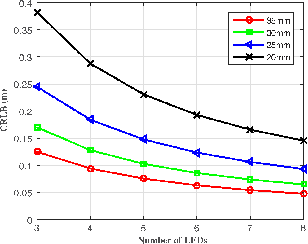

Finally, we investigate how CRLB behaves as we vary the frame rate of the camera receiver. In Fig. 10, the CRLB is plotted versus the number of LEDs for various frame rates. It shows that for a given number of LEDs, the CRLB drops with reducing frame rate. For four LEDs used in the outdoor IS-based VLP system at a communication distance of 30 m between the LED array transmitter and the camera receiver, the CRLB of the position of camera receiver for the frame rate of 1000 fps is about 0.5 m. This falls to only about 0.05 m when the frame rate is decreased to 30 fps. Therefore, the positioning accuracy increases with reducing of the frame rate, However, the lower frame rate (which is equal to the sampling rate of the camera IS) directly limits the achievable data rate. This is the reason why high speed cameras are usually utilized for VLC, while medium and low speed cameras are used for VLP.

Fig. 10

Influence of frame rate on CRLB with the frame rate from 30 to 1000 fps. The communication distance between the LED array transmitter and the camera receiver is 30 m, and the camera receiver has a focal length of 35 mm and a pixel width of $10 μ m$ .

6. Conclusion

For a typical outdoor scenario, theoretical limits of the location of an in-vehicle camera receiver are calculated by deriving the CRLB. Under the condition that the observation values of the LED imaging points are affected by white Gaussian noise, the MLE for the vehicle position is first calculated, then the CRLB is derived. For typical parameters of a white LED array and in-vehicle camera IS, simulation results show that accurate location estimation is achievable, with the positioning error usually in the order of centimeters for a communication distance of 30 m between the LED array transmitter and the camera receiver. Positioning accuracy has relation with the number of LEDs used, the focal length of the lens, and the pixel size and frame rate of the camera receiver in the presence of a constant communication distance. The determination of the CRLB will provide a theoretical basis of statistical analysis for the optimization problem for outdoor IS-based VLP systems.

Acknowledgments

This work was supported by the Natural Science Foundation of China under Grant Nos. 61261017, 61362006, and 61371107, the Natural Science Foundation of Guangxi under Grant Nos. 2014GXNSFAA118387 and 2013GXNSFAA019334, the Key Laboratory Foundation of Guangxi Broadband Wireless Communication and Signal Processing under Grant No. GXKL061501, the Guangxi Colleges and Universities Key Laboratory Foundation of Intelligent Processing of Computer Images and Graphics under Grant No. GIIP201407, and the High-Level Innovation Team of New Technology on Wireless Communication in Guangxi Higher Education Institutions.

References

1.

P. Pathak et al., “Visible light communication, networking, and sensing: a survey, potential and challenges,” IEEE Commun. Surv. Tutorials, 17 2047 –2077 (2015). http://dx.doi.org/10.1109/COMST.2015.2476474 Google Scholar

2.

S. Arnon, Visible Light Communication, Cambridge University Press, Cambridge, United Kingdom (2015). Google Scholar

3.

D. Karunatilaka et al., “LED based indoor visible light communications: state of the art,” IEEE Commun. Surv. Tutorials, 17 1649 –1678 (2015). http://dx.doi.org/10.1109/COMST.2015.2417576 Google Scholar

4.

H. Li et al., “An analog modulator for 460 mb/s visible light data transmission based on OOK-NRS modulation,” IEEE Wireless Commun., 22 68 –73 (2015). http://dx.doi.org/10.1109/MWC.2015.7096287 Google Scholar

5.

Q. Gao et al., “DC-informative joint color-frequency modulation for visible light communications,” J. Lightwave Technol., 33 2181 –2188 (2015). http://dx.doi.org/10.1109/JLT.2015.2420658 JLTEDG 0733-8724 Google Scholar

6.

W. Huang, C. Gong and Z. Xu, “System and waveform design for wavelet packet division multiplexing-based visible light communications,” J. Lightwave Technol., 33 3041 –3051 (2015). http://dx.doi.org/10.1109/JLT.2015.2491962 JLTEDG 0733-8724 Google Scholar

7.

Y. Wang et al., “4.5-Gb/s RGB-LED based WDM visible light communication system employing CAP modulation and RLS based adaptive equalization,” Opt. Express, 23 13626 –13633 (2015). http://dx.doi.org/10.1364/OE.23.013626 OPEXFF 1094-4087 Google Scholar

8.

N. U. Hassan et al., “Indoor positioning using visible led lights: a survey,” ACM Comput. Surv., 48 20:1 –20:32 (2015). http://dx.doi.org/10.1145/2830539 ACSUEY 0360-0300 Google Scholar

9.

T. Yamazato and S. Haruyama, “Image sensor based visible light communication and its application to pose, position, and range estimations,” IEICE Trans. Commun., E97-B 1759 –1765 (2014). http://dx.doi.org/10.1587/transcom.E97.B.1759 Google Scholar

10.

J. Armstrong, Y. Sekercioglu and A. Neild, “Visible light positioning: a roadmap for international standardization,” IEEE Commun. Mag., 51 68 –73 (2013). http://dx.doi.org/10.1109/MCOM.2013.6685759 ICOMD9 0163-6804 Google Scholar

11.

U. Nadeem et al., “Indoor positioning system designs using visible LED lights: performance comparison of TDM and FDM protocols,” Electron. Lett., 51 (1), 72 –74 (2015). http://dx.doi.org/10.1049/el.2014.1668 ELLEAK 0013-5194 Google Scholar

12.

J. Lim, “Ubiquitous 3D positioning systems by led-based visible light communications,” IEEE Wireless Commun., 22 80 –85 (2015). http://dx.doi.org/10.1109/MWC.2015.7096289 Google Scholar

13.

M. Yasir, S.-W. Ho and B. Vellambi, “Indoor positioning system using visible light and accelerometer,” J. Lightwave Technol., 32 3306 –3316 (2014). http://dx.doi.org/10.1109/JLT.2014.2344772 JLTEDG 0733-8724 Google Scholar

14.

U. Nadeem et al., “Highly accurate 3D wireless indoor positioning system using white LED lights,” Electron. Lett., 50 828 –830 (2014). http://dx.doi.org/10.1049/el.2014.0353 ELLEAK 0013-5194 Google Scholar

15.

G. Prince and T. Little, “A two phase hybrid RSS/AoA algorithm for indoor device localization using visible light,” in 2012 IEEE Global Communications Conf. (GLOBECOM ‘12), 3347 –3352 (2012). http://dx.doi.org/10.1109/GLOCOM.2012.6503631 Google Scholar

16.

K. Panta and J. Armstrong, “Indoor localisation using white LEDs,” Electron. Lett., 48 228 –230 (2012). http://dx.doi.org/10.1049/el.2011.3759 ELLEAK 0013-5194 Google Scholar

17.

S.-Y. Jung, S. Hann and C.-S. Park, “TDOA-based optical wireless indoor localization using LED ceiling lamps,” IEEE Trans. Consum. Electron., 57 1592 –1597 (2011). http://dx.doi.org/10.1109/TCE.2011.6131130 ITCEDA 0098-3063 Google Scholar

18.

A. Ohmura et al., “Accuracy improvement by phase only correlation for distance estimation scheme for visible light communications using an LED array and a high-speed camera,” in 20th World Congress on Intelligent Transport Systems, (2013). Google Scholar

19.

M. Yoshino, S. Haruyama and M. Nakagawa, “High-accuracy positioning system using visible LED lights and image sensor,” in 2008 IEEE Radio and Wireless Symp., 439 –442 (2008). http://dx.doi.org/10.1109/RWS.2008.4463523 Google Scholar

20.

M. Rahman, M. Haque and K.-D. Kim, “High precision indoor positioning using lighting LED and image sensor,” in 14th Int. Conf. on Computer and Information Technology (ICCIT ‘11), 309 –314 (2011). http://dx.doi.org/10.1109/ICCITechn.2011.6164805 Google Scholar

21.

C. Barberis et al., “Experiencing indoor navigation on mobile devices,” IT Prof., 16 50 –57 (2014). http://dx.doi.org/10.1109/MITP.2013.54 Google Scholar

22.

I. Takai et al., “Optical vehicle-to-vehicle communication system using LED transmitter and camera receiver,” IEEE Photonics J., 6 1 –14 (2014). http://dx.doi.org/10.1109/JPHOT.2014.2352620 Google Scholar

23.

R. Roberts, “Automotive comphotogrammetry,” in IEEE 79th Vehicular Technology Conf. (VTC Spring ‘14), 1 –5 (2014). http://dx.doi.org/10.1109/VTCSpring.2014.7022840 Google Scholar

24.

T. Yamazato et al., “Image sensor-based visible light communication for automotive applications,” IEEE Commun. Mag., 52 88 –97 (2014). http://dx.doi.org/10.1109/MCOM.2014.6852088 ICOMD9 0163-6804 Google Scholar

25.

T. Yamazato et al., “Vehicle motion and pixel illumination modeling for image sensor based visible light communication,” IEEE J. Sel. Areas Commun., 33 1793 –1805 (2015). http://dx.doi.org/10.1109/JSAC.2015.2432511 Google Scholar

26.

S. Haruyama, “Advances in visible light communication technologies,” in 38th European Conf. and Exhibition on Optical Communications (ECOC ‘12), 1 –3 (2012). Google Scholar

27.

R. Gow et al., “A comprehensive tool for modeling CMOS image-sensor-noise performance,” IEEE Trans. Electron Devices, 54 1321 –1329 (2007). http://dx.doi.org/10.1109/TED.2007.896718 IETDAI 0018-9383 Google Scholar

28.

J. Kahn and J. Barry, “Wireless infrared communications,” Proc. IEEE, 85 265 –298 (1997). http://dx.doi.org/10.1109/5.554222 Google Scholar

29.

S. M. Kay, Fundamentals of Statistical Signal Processing, Prentice Hall, Upper Saddle River, New Jersey (1993). Google Scholar

30.

R. Zekavat and R. M. Buehrer, Handbook of Position Location: Theory, Practice and Advances, Wiley-IEEE Press, Hoboken, New Jersey (2011). Google Scholar

Biography

Xiang Zhao received her BS degree in information engineering and her MS degree in communication and information systems from Guilin University of Electronic Technology, Guilin, China, in 2001 and 2006, respectively. She is currently working toward her PhD in communication and information systems from Xidian University, Xian, China, and her current research interests are visible light communication and visible light positioning.

Jiming Lin received his MSc degree from the University of Electronic Science and Technology of China in 1995 and his PhD from Nanjing University in 2002. Then he held a two-year postdoctoral fellowship at the State Key Laboratory for Novel Software Technology at Nanjing University. Since 2004, he has been a professor of Guilin University of Electronic Technology. His research interests are in synchronization and localization in WSNs, UWB communication, and visible light communication and positioning.

CC BY: © The Authors. Published by SPIE under a Creative Commons Attribution 4.0 Unported License. Distribution or reproduction of this work in whole or in part requires full attribution of the original publication, including its DOI.

Citation Download Citation

Xiang Zhao and Jiming Lin "Maximum likelihood estimation of vehicle position for outdoor image sensor-based visible light positioning system," Optical Engineering 55(4), 043104 (18 April 2016). https://doi.org/10.1117/1.OE.55.4.043104

Published: 18 April 2016

Access the abstract

JOURNAL ARTICLE
8 PAGES

DOWNLOAD PAPER SAVE TO MY LIBRARY

GET CITATION

CITATIONS

Cited by 5 scholarly publications.

Explore citations on Lens.org

KEYWORDS

Light emitting diodes

Cameras

Receivers

Imaging systems

Transmitters

Image sensors

Visible radiation

1.

Introduction

2.

System Model

Fig. 1

Table 1

Eq. (1)

Eq. (2)

Fig. 2

Eq. (3)

Eq. (4)

3.