Energy flow: image correspondence approximation for motion analysis

Liangliang Wang; Ruifeng Li; Yajun Fang

doi:10.1117/1.OE.55.4.043109

29 April 2016 Energy flow: image correspondence approximation for motion analysis

Liangliang Wang, Ruifeng Li, Yajun Fang

Author Affiliations +

Optical Engineering, Vol. 55, Issue 4, 043109 (April 2016). https://doi.org/10.1117/1.OE.55.4.043109

Abstract

We propose a correspondence approximation approach between temporally adjacent frames for motion analysis. First, energy map is established to represent image spatial features on multiple scales using Gaussian convolution. On this basis, energy flow at each layer is estimated using Gauss–Seidel iteration according to the energy invariance constraint. More specifically, at the core of energy invariance constraint is “energy conservation law” assuming that the spatial energy distribution of an image does not change significantly with time. Finally, energy flow field at different layers is reconstructed by considering different smoothness degrees. Due to the multiresolution origin and energy-based implementation, our algorithm is able to quickly address correspondence searching issues in spite of background noise or illumination variation. We apply our correspondence approximation method to motion analysis, and experimental results demonstrate its applicability.

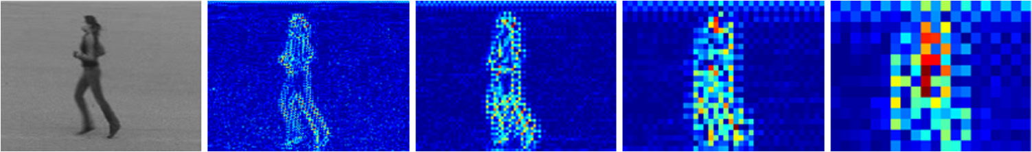
1. Introduction

Motion analysis is a very significant topic in computer vision because of its demand in the area of human–computer interaction, video surveillance, intelligent transportation system, and others. As motion is a time-varying quantity reflecting the variation of an object’s status, in contrast to static image analysis, more useful changing information is available via spatial feature comparison between frames for motion analysis.¹^,² Therefore, at the center of motion analysis is to represent different motions according to their dissimilarities in space-time. From this perspective, techniques for analyzing motion can be divided into two categories: spatial dissimilarity-oriented and temporal dissimilarity-oriented methods.

To be definite, we regard spatial dissimilarity-oriented methods as techniques focusing on exploring dissimilarities of image features, and then combine or extend by adding time labels for motion representation. As a good example, Gilbert and Bowden³ proposed a dense interest points detection algorithm for human action feature extraction, which is further temporally grouped for classification. Recently, spatiotemporal shape template⁴^–⁷ for motion representation attracts much attention for its effectiveness; however, the templates rely strongly on spatial shape representation. Similarly, approaches based on bag of spatiotemporal interest points⁸^–¹¹ has great success in the field of motion analysis for its space-time invariance. Generally, in spite of spatial dissimilarity-oriented methods being very suitable for motion representation where spatial characteristics are obvious, they often fail to extract adequate global relationships of motion.

In contrast, temporal dissimilarity-oriented methods tend to first extract image features, and then focus on exploiting the relationship and dissimilarities between motion frames. Frame difference is a very direct and useful scheme to express motion temporal dissimilarities. For example, in Ref. 12, motion energy image (MEI) is built up through image difference, based on which motion history image is formulated by fusing MEI for human movement recognition. Moreover, optical flow¹³ is another popular temporal dissimilarity-oriented scheme by assuming brightness is constant between adjacent frames. Inspired by optical flow, Liu and Torralba¹⁴ developed scale-invariant feature transform (SIFT) flow using SIFT points substituting raw pixels for dense correspondence analysis, which is further applied for motion field prediction and face recognition. Furthermore, Huang et al.¹⁵ presented a correspondence map-based algorithm which can be employed for object recognition. Generally speaking, temporal dissimilarity-oriented methods cover both global and local features of motion, and many attempts have been made to address the motion analysis problem from the perspective of image correspondence approximation, as it is more accessible and applicable than frame difference techniques in most cases.

Motivated by the aforementioned observations, this paper solves the motion analysis problem by developing an image correspondence approximation scheme called energy flow, which can be used for dissimilarity searching in space-time between temporally adjacent frames. Particularly, our work first generates a multiscale energy map for image spatial effective representation, which allows for image detail preservation while extracting main features. Using energy map, energy flow at each scale is computed by Gauss–Seidel iteration based on the energy invariance constraint as well as global smoothness assumption.¹⁶ Ultimately, we reconstruct an energy flow field on different scales for accurate image correspondence approximation.

The proposed scheme is capable of finding out dissimilarities between two images, which has great prospect in computer vision domain. Compared with optical flow techniques,¹³ our algorithm is more reliable and has higher tolerance to illumination changes since multiscale energy rather than brightness is employed for pattern flow searching. As the application for motion analysis, our approach is very practical in contrast to SIFT flow¹⁴ and other spatialtemporal representation methods, for its cheap and accessible characteristics.

The remainder of this paper is organized as follows. Sec. 2 gives an overview of related work. In Sec. 3, our energy flow concept is introduced. Section 4 shows the motion analysis results using energy flow. Finally, Sec. 5 concludes this paper.

2. Related Work

As energy flow is an image correspondence-based scheme, as well, motion analysis is a very broad topic allied closely with image segmentation, background modeling, tracking, object recognition, and others, we review previous work from three aspects: image correspondence, motion detection, and human action recognition.

2.1.

Image Correspondence Approximation

Initially, Horn and Schunck¹⁶ proposed an optical flow estimation method to find dense correspondence fields between images. Optical flow is very efficient for small motions, so a great deal of research¹³^,¹⁷^,¹⁸ following this pipeline has been done for correspondence approximation. However, optical flow makes the brightness constancy assumption and therefore fails to deal with large lighting changes, it also cannot accurately describe the motion region if there is overlap or noise on the brightness layer.

Another popular image correspondence technique is SIFT,¹⁹ which matches the images using sparse points that are robust to geometric and photometric variations on multiple scales. SIFT flow,¹⁴ mentioned earlier, is actually an extension of SIFT by fusing it into optical flow formulation. Unfortunately, SIFT-based algorithms are either computationally consuming or too sparse to achieve precise correspondence approximation. To deal with these shortcomings, Tau and Hassner²⁰ further seek to propagate image scale information from detected interest points to its neighboring pixels context by considering locations where scales are detected, and then use the context for images separately and within correlated images, which results in more useful features for dense correspondence while keeping the computational burden low. Similarly, Zhang et al.²¹ proposed an energy flow equation by replacing the brightness using image temperature features within the Horn–Schunck optical flow framework, which is employed for video segmentation.

Moreover, researchers present many approaches for approximating image correspondence from other points of view, such as Refs. 15 and 22, no matter if they work on pixels or interest points, the dilemma between accuracy and efficiency is challenging especially for wide-range practical applications.

2.2.

Motion Detection

Broadly speaking, existing work for motion detection can be roughly divided into model-based and appearance-based detections. Model-based methods detect motions by comparing the target with a built model. It is ideal to directly use the background image²² without interference as the model if the scenario is static, but more often, using an estimated model from a priori knowledge is more actual, e.g., Gaussian mixture model (GMM)²³ is proposed for dynamic model estimation according to the Gaussian mixture distribution of pixels, which is widely applied for object tracking. In a very recent work, Haines and Xiang²⁴ further used a Dirichlet process GMM to provide a per-pixel density estimate for background computation. Model-based techniques are quick, but rely strongly on the established model. Appearance-based approaches pay more attention to learn a large number of sample features, and then accomplish motion detection by classification, e.g., histogram of oriented gradient (HOG)²⁵ is formulated to represent gradient features of an image, according to which, pedestrians can be detected via support vector machines (SVMs) framework.²⁶ In Ref. 4, a detector named action bank is presented for human motion detection, and on this basis, motion can be accurately localized through SVMs. Tamrakar et al.¹⁰ introduced a bag of SIFT features for complex event detection.

2.3.

Human Action Recognition

As human action is a very large-volume data digitally, the heart of action recognition is to extract spatiotemporal features³ to represent actions. Considering the characteristics of action, many action descriptors have been presented, e.g., Derpanis et al.⁶ developed a spatial-temporal orientation template generated via three-dimensional Gaussian filtering on raw raw image intensity features for reflecting the dynamics of actions. In Ref. 7, action videos are segmented into spatiotemporal graphs expressing hierarchical, temporal, and spatial relationships of actions, and then a matching algorithm is formulated for action recognition. Additionally, a lot of techniques originated from image correspondence and motion detection are widely applied for action recognition, e.g., Laptev et al.⁸ build a spatiotemporal bag of words (BoW) model to represent action interest points consisting of HOG and optical flow features. Furthermore, context of interest points is able to be used for action representation, e.g., in Ref. 27, the action context feature is defined as the relative coordinates of pairwise interest points in space-time, and then GMMs are used to describe the context distributions of interest points.

3. Methodology

Our goal is to explore correspondence between images for motion analysis. In this work, a temporal dissimilarity-oriented scheme is presented while the spatial features of images are deep extracted. Given two temporally adjacent frames, we start from building multilayer Laplacian stacks for both, respectively, using Gaussian kernel convolution implementation, and energy map is further established for image feature extraction. We compute the energy flow between two energy maps based on the energy invariance constraint, and energy flow field is reconstructed to approximate the correspondence.

3.1.

Energy Map

To exploit the local features of an image, the first step of our algorithm is to represent an image $I$ on multiple scales employing Laplacian stacks. Let $G (σ)$ denote a two-dimensional normalized Gaussian kernel with standard deviation $σ$ , and let $*$ denote the convolution operator, the image $I$ can be decomposed into a $m$ -scale ( $m \geq 1$ ) descriptor ${L_{S} (I) | 0 \leq S \leq m}$ , where

Eq. (1)

L_{S} (I) = {\begin{cases} I - I * G (σ) & if S = 0 \\ I * G (σ^{S}) - I * G (σ^{S + 1}) & if S > 0 \end{cases} .

Despite the fact that Laplacian stacks are able to find out full details as its origin at multiresolution processing, for each subband, it is band limited.²⁸ Therefore, in order to describe an image more accurately with fewer noises by considering the dissimilarity between different scales, a rectification process is implemented in our work. Based on the Laplacian stacks, and inspired by power maps proposed in Refs. 22 and 28, we establish our energy map according to the absolute value of Laplacian coefficients because the variation produced by difference of Laplacian stacks rather than its orientation is the point of our concern. For $I$ on the $S$ ’th scale, we define the transfer energy as

Eq. (2)

T_{S} (I) = \ln | L_{S} (I) | * G (σ^{S + 1}) .

Here, we transform the absolute value of Laplacian coefficients into logarithmic domain. Since the value of $| L_{S} (I) |$ at many pixels is 0, which brings infinitely small quantity impacting the following computation, we make the following revision:

Eq. (3)

T_{S}^{'} (I) = \ln | L_{S}^{'} (I) | * G (σ^{S + 1}),

where

Eq. (4)

| L_{S}^{'} (I) | = {\begin{cases} | L_{S} (I) | & if | L_{S} (I) | \neq 0 \\ 1 & if | L_{S} (I) | = 0 \end{cases} .

Then we continue to define the energy map considering both the absolute value of $L_{S} (I)$ and the exponent of weighted transfer energy:

Eq. (5)

E_{S} (I) = | L_{S} (I) | e^{λ T_{S}^{'} (I)},

where

λ

is an adaptable parameter. Since the revision process adds noises to

e^{λ T_{S}^{'} (I)}

by conserving zeros of

| L_{S} (I) |

, we further modify it using

P_{S} (I)

:

Eq. (6)

P_{S} (I) = {\begin{cases} e^{λ T_{S}^{'} (I)} & if | e^{λ T_{S}^{'} (I)} - e^{λ ρ} | > ε \\ 0 & else \end{cases},

where

ε

is the infinitely small quantity, and

ρ

is a parameter determined by image quality.

Finally, energy map is built up as follows:

Eq. (7)

E_{S} (I) = | L_{S} (I) | P_{S} (I) .

Thus, we can conclude that our energy map is essentially the multilayer Laplacian energy stacks for action spatial feature extraction. Figure 1 shows an example of energy map, it is worth noting that the four layers of energy map are displayed with the same size in spite of actually every backward layer decreases into one-fourth with respect to its forward layer. Additionally, it is worth noting that $σ$ is set as 2, $m$ is chosen as 4, $λ$ is selected as $- 0.3$ , and $ρ$ ranges from $- 2$ to $- 0.5$ in our work which are practically proven to work well.

Fig. 1

An example of energy map. The first column is the initial action image, and from the second to the fifth columns are the energy maps on four layers, respectively.

3.2.

Energy Flow

To extract temporal features between frames, we regard motion as the apparent motion of the energy. Therefore, as we know, there are two smoothness assumptions¹³ for optical flow computation: global smoothness¹⁶ which can produce dense optical flow field but fail to describe boundaries and local smoothness¹⁷ which is more robust but often results in sparse motion description. Considering the advantage of the energy map on depicting boundaries, and motivated by Horn–Schunck optical flow formulation,¹⁶ we make the assumption that the spatial energy at two continuous times on the same scale is equal using global smoothness assumption. Moreover and likewise, we define “energy conservation law” as follows: let $E_{S} (x, y, t)$ denote the energy of a pixel $(x, y)$ of an image $I$ at time $t$ on the $S$ ’th scale, after a small time interval $δ t$ at the point $(x + δ x, y + δ y)$ , we thus define

Eq. (8)

E_{S} (x, y, t) = E_{S} (x + δ x, y + δ y, t + δ t) .

Based on this assumption, we expand the above equation using Taylor series:

Eq. (9)

E_{S} (x, y, t) + δ x \frac{\partial E_{S}}{\partial x} + δ y \frac{\partial E_{S}}{\partial y} + δ t \frac{\partial E_{S}}{\partial t} + o (2) = E_{S} (x, y, t),

where

o (2)

denotes the first-order of infinitely small quantity. Then dividing

δ t

on both sides of Eq. (9), and as

δ t \to 0

, we can get

Eq. (10)

\frac{\partial E_{S}}{\partial x} \frac{d x}{d t} + \frac{\partial E_{S}}{\partial y} \frac{d y}{d t} + \frac{\partial E_{S}}{\partial t} = 0 .

Here, we define the velocity of a pixel as $ν_{S} = (ν_{S x}, ν_{S y})$ and $ν_{S x} = (d x / d t)$ , $ν_{S y} = (d y / d t)$ , so we can get the energy flow constraint equation:

Eq. (11)

\frac{\partial E_{S}}{\partial x} ν_{S x} + \frac{\partial E_{S}}{\partial y} ν_{S y} + \frac{\partial E_{S}}{\partial t} = 0 .

Then we describe energy flow using the energy flow field descriptor $ν_{S} = (ν_{S x}, ν_{S y})$ , which can be computed by minimizing the following objective function:

Eq. (12)

ν_{S} = \underset{ν_{S}}{argmin} \sum_{x} [α_{1} {‖ \frac{\partial E_{S}}{\partial x} ν_{S x} + \frac{\partial E_{S}}{\partial y} ν_{S y} + \frac{\partial E_{S}}{\partial t} ‖}^{2} + α_{2} ({‖ \frac{\partial ν_{S}}{\partial x} ‖}^{2} + {‖ \frac{\partial ν_{S}}{\partial y} ‖}^{2})],

where

α_{1} (α_{1} \neq 0)

and

α_{2}

are respectively the weights for data and smoothness terms indicating the energy invariance and global smoothness assumption.¹³ Likewise, the ratio

α_{2} / α_{1}

is determined by the image quality.²⁹

Utilizing the Gauss–Seidel iteration, Eq. (12) can be solved as follows:

Eq. (13)

ν_{S x}^{k + 1} = {\bar{ν}}_{S x}^{k} - \frac{\frac{\partial E_{S}}{\partial x} {\bar{ν}}_{S x}^{k} + \frac{\partial E_{S}}{\partial y} {\bar{ν}}_{S y}^{k} + \frac{\partial E_{S}}{\partial t}}{{(\frac{α_{2}}{α_{1}})}^{2} + {(\frac{\partial E_{S}}{\partial x})}^{2} + {(\frac{\partial E_{S}}{\partial y})}^{2}} \frac{\partial E_{S}}{\partial x},

Eq. (14)

ν_{S y}^{k + 1} = {\bar{ν}}_{S y}^{k} - \frac{\frac{\partial E_{S}}{\partial x} {\bar{ν}}_{S x}^{k} + \frac{\partial E_{S}}{\partial y} {\bar{ν}}_{S y}^{k} + \frac{\partial E_{S}}{\partial t}}{{(\frac{α_{2}}{α_{1}})}^{2} + {(\frac{\partial E_{S}}{\partial x})}^{2} + {(\frac{\partial E_{S}}{\partial y})}^{2}} \frac{\partial E_{S}}{\partial y},

where

k (k \geq 0)

denotes the iteration number, and in our work,

k

is set as 100 to guarantee both efficiency and accuracy.

3.3.

Energy Flow Field Reconstruction

Therefore, after iteration via Eqs. (13) and (14), from the macropoint of view, for two frames, we can get a final energy flow field sequence abbreviated as ${V_{S} = (ν_{S x}^{k + 1}, ν_{S y}^{k + 1}) | 0 \leq S \leq m}$ on multiple scales. Because for high-pass scales, the energy map averages response over a larger region of the image;²⁸ to represent the details produced by tiny variation during the time interval $δ t$ and to guarantee the avoidance of noise simultaneously, we reconstruct energy flow field on the velocity layer rather than on the energy map layer for expressing image correspondence relationship using $V_{0}$ , which can be computed by iteration as follows:

Eq. (15)

V_{S} = {\begin{cases} V_{S} & if S = m \\ V_{S} + \frac{S + 1}{S + 2} V_{S + 1} * G (σ^{S + 1}) & if S < m \end{cases} .

4. Experiments

As our algorithm is an image correspondence-based scheme for dissimilarity searching between adjacent frames, to better reveal its performance, we test our algorithm for motion analysis from two facets: motion detection and human action recognition. Also, we believe that our method can be used in more areas.

4.1.

Motion Detection

We verify our algorithm for motion field prediction using frames from ChangeDetection.NET 2014 change detection database³⁰ without additional processing. ChangeDetection. Net 2014 is a very complex benchmark for event and motion detection consisting of 31 videos depicting indoor and outdoor scenes with boats, cars, trucks, and pedestrians.

To visualize energy flow velocities, we display oriented arrows of energy flow field from the previous frame to the current status, and one velocity vector in $2 \times 2$ or $5 \times 5 pixels$ is set to be visible and the magnifying scale factor of arrows is 5 or 10 determined by image quality. As well, we utilize color maps to show energy flow field regions according to the value of $\arctan (ν_{0 x}^{101} / ν_{0 y}^{101})$ at each pixel, it is worth noting that the previous frames are often not given but can be inferred from our visualizations which reflect motion variations.

Figure 2 gives the example results of continuous human motion detection in a relatively static scenario, the grabbing motion is slow, a large part of the human body is not moving, and a small part moves slightly. From detection results, we can see that our algorithm is able to depict moving parts effectively with little noises and the boundaries are precisely detected. Also, the overlap within motions is successfully addressed.

Fig. 2

Example results of human motion detection. Images in the top row are continuous frames with oriented arrows describing energy flow velocities from its previous frame to the current status, and the bottom row shows the color maps. The previous frame of the first image is not given.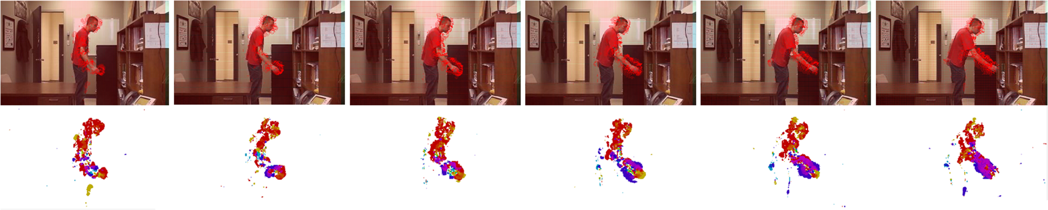

Figure 3 gives the example results of motion detection in the lake and highway scenarios. The lake scenario is very challenging as it includes motions of a man driving a boat, a black car’s motion far away from lens, and the lake water flow. However, we deal with the case well and the main motion variations are detected. For the highway scenario, the motion is very quick leading to big variations, and it is shown from the results that the motions are localized very accurately, but a part of the car’s body is disregarded.

Fig. 3

Example results of motion detection in the lake and highway scenarios. Images in the top row are representative frames with oriented energy flow arrows, and the bottom row shows the corresponding color maps.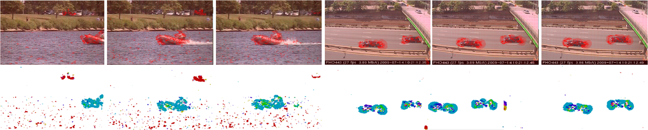

Figure 4 gives the example results of motion detection in a shadow scenario and at night. The results of pedestrian detection with shadow are promising since we are aimed at motion detection instead of detecting pedestrians. As motion detection at night with illumination changes, our approach is also very robust.

Fig. 4

Example results of motion detection in a shadow scenario and at night. Images in the top row are representative frames with oriented energy flow arrows, and the bottom row shows the corresponding color maps.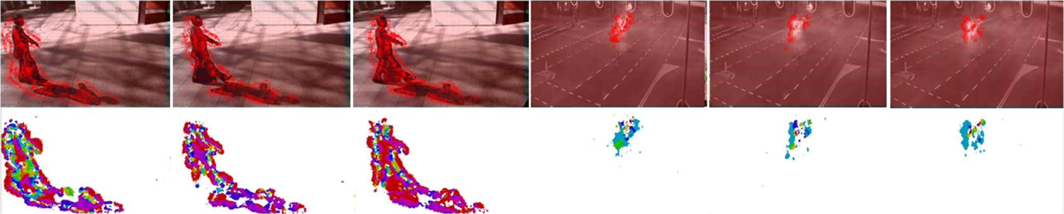

As a comparison, Fig. 5 compares our method with optical flow methods of Refs. 16 and 17 using color map on examples from ChangeDetection. Net 2014. Between two frames of human walking with a box, the main motion lies on wiggling of the foot behind and translation of the upper body, and from the results, we can see that the method of Ref. 16 cannot describe boundaries accurately and is heavily damaged by noise; the method of Ref. 17 enlarges the motion part and is not reliable in contrast to our approach. Moreover, the average running time of our algorithm for 10 times is 0.039 s, compared with 17.143 and 0.918 s by methods of Refs. 17 and 16. We implement all the experiments in MATLAB on an i5-core PC with a 6 GB RAM.

Fig. 5

Example results of pedestrian detection on ChangeDetection. Net 2014 database using energy flow and optical flow methods (respectively proposed by Horn and Mahmoudi).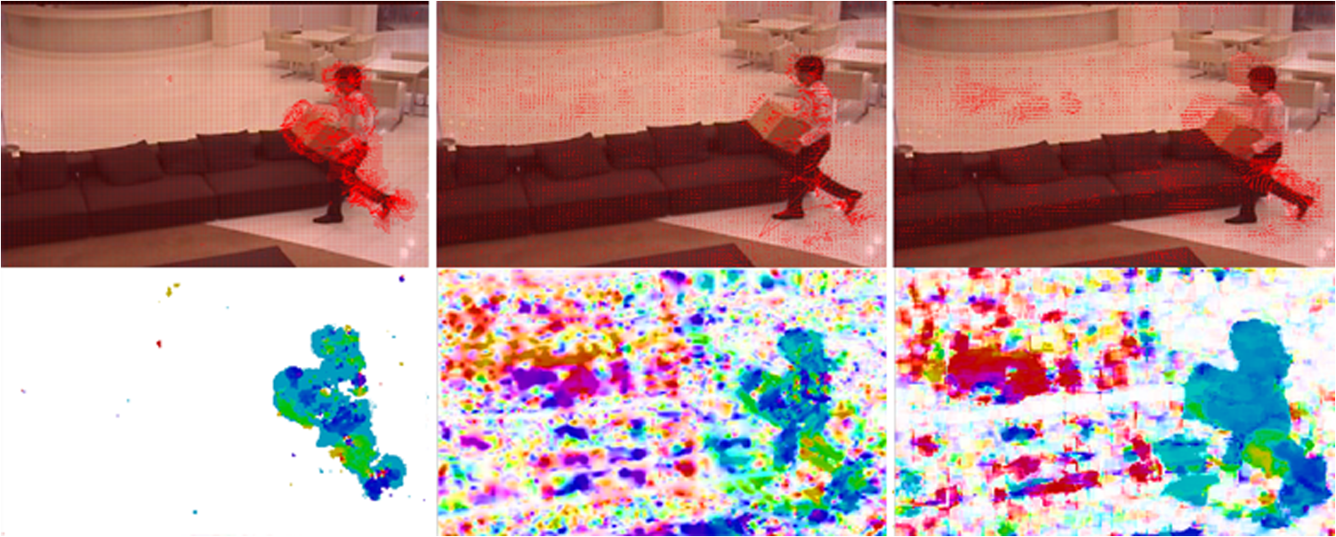

Moreover, to further validate our approach, we compare its overall results with another four methods for motion detection on ChangeDetection. Net 2014 shown in Table 1. We select three popular metrics for evaluation: recall ( $R e = N_{t p} / N_{t p} + N_{f n}$ ), false positive rate [ $F p r = N_{f p} / (N_{f p} + N_{t n})$ ], and precision [ $P r = N_{t p} / (N_{t p} + N_{f p})$ ], which are determined by the number of true positives ( $N_{t p}$ ), true negatives ( $N_{t n}$ ), false positives ( $N_{f p}$ ), and false negatives ( $N_{f n}$ ). From the comparison, we can see that our method outperforms popular optical flow methods,¹⁶^,¹⁷ and can handle real-time action detection well in contrast to GMM²³ and background modeling²⁴ based algorithms.

Table 1

Overall action detection results of different algorithms on ChangeDetection. Net 2014 database.

Method	Re	Fpr	Pr
Horn and Schunck¹⁶	0.68	0.030	0.56
Mahmoudi et al.¹⁷	0.69	0.022	0.65
Stauffer and Grimson²³	0.62	0.025	0.60
Haines and Xiang²⁴	0.78	0.013	0.74
Our algorithm	0.76	0.009	0.81

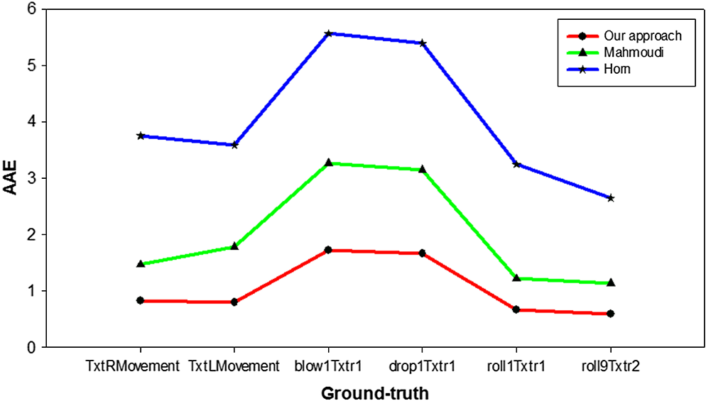
To evaluate our energy flow errors, we compute average angular errors (AAE) of energy flow using ground-truth sequences (“TxtRMovement,” “TxtLMovement,” “blow1Txtr1,” “drop1Txtr1,” “roll1Txtr1,” and “roll9Txtr2”) from University College London (UCL) database¹⁸ by averaging all the $A E$ calculated by the following equation:

Eq. (16)

A E = \cos^{- 1} [\frac{1 + ν_{0 x}^{101} \times ν_{x} + ν_{0 x}^{101} \times ν_{y}}{\sqrt{1 + {(ν_{0 x}^{101})}^{2} + {(ν_{0 x}^{101})}^{2}} \sqrt{1 + ν_{x}^{2} + ν_{y}^{2}}}],

where

(ν_{x}, ν_{y})

denotes the velocity of ground-truth at

(x, y)

. As a comparison, the AAE of Refs. 16 and 17 is also shown in Fig. 6.

Fig. 6

AAE of different methods using ground-truth from UCL database.

4.2.

Human Action Recognition

For action recognition issue, we select sequences from Kungl Tekniska Högskolan (KTH) (2391 video clips including 6 actions performed by 25 persons)²⁶ and human metabolome database (HMDB) (6849 video clips divided into 51 action categories)³¹ action databases. Using energy flow field between two frames as features, we cluster $100 k$ features of the energy flow field descriptors using $k$ -means algorithm by setting $k$ as 4000, then encode them via a BoW as depicted in Ref. 10, and finally we classify actions under SVMs framework with radial basis function kernel which is practically demonstrated robust. For each action, same as in Refs. 26 and 31, we select 16 persons’ video clips for training and the rest for testing on KTH, while we choose 70 video clips for training and 30 video clips for testing on HMDB.

Figure 7 gives the confusion matrix using our method on KTH database, and the average recognition rate (ARR) reaches 93.65%. Table 1 compares our algorithm with other related works.⁶^,¹¹^,²³^,²⁶ In the meanwhile, with the same settings except using SIFT³¹ and optical flow features¹⁷ replacing our energy flow features, we get the ARR which is shown in Table 2.

Table 2

ARR of different methods on KTH database.

Method	ARR
Schuldt and Caputo²⁶	71.7
Derpanis et al.⁶	89.34
Laptev et al.⁸	91.8
Iosifidis and Pitas¹¹	92.13
SIFT + BoW	85.46
Optical flow + BoW	79.59
Our algorithm	93.65

Fig. 7

Confusion matrix of our algorithm on KTH dataset.

Table 3 shows the recognition results of our approach (ARR is 27.92%) and others²⁶^,³²^,³³ on HMDB database. Also we substitute energy flow using optical flow and SIFT features for comparison, and the corresponding recognition rates are also given. From experimental results, we can see that our method is very effective.

Table 3

ARR of different methods on HMDB database.

Method	ARR
Kuehne²³	23.18
Sadanand and Corso⁴	26.9
Cao et al.⁵	27.84
SIFT + BoW	21.56
Optical flow + BoW	16.87
Our algorithm	27.92

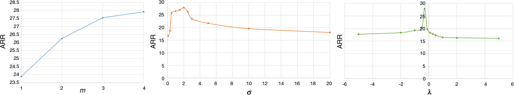
Finally, we record different ARRs on HMDB database by setting different parameters of $m$ , $σ$ , and $λ$ in Fig. 8. We can observe that both the standard deviation $σ$ and the threshold $λ$ perform well in a limited range, which verifies that noises would contaminate the contributing data if parameters are too small while useful information would be omitted if too large. Also, the layer of Laplacian stacks $m$ should be chosen as large as possible if the resolution of image permits. Note that we change only one parameter’s value while setting others as default in our experiments.

Fig. 8

Evaluation of different parameters for action recognition on HMDB database.

5. Conclusion

In this paper, we present an image correspondence framework for motion analysis by estimating energy flow field between two adjacent frames. Energy map is introduced for image feature extraction, based on which energy invariant constraint is proposed for energy flow calculation. The reconstructed energy flow field considering the smoothness degrees of multiple scales is applied for both motion field prediction and human action recognition. A number of experiments are carried out, and promising results are given.

Energy flow scheme is very suited for real-time motion analysis regardless of background noise or illumination change. However, we also find a limitation: in some cases, we may lose a part of specific energy flow field within the object’s boundaries due to the poor image quality. So, additional postprocessing should be considered if the whole motion silhouette is needed. In our future work, we are very interested in applying our approach into more computer vision fields.

Acknowledgments

This research was supported by the National Natural Science Foundation of China (Grant No. 661273339). The authors also would like to thank Berthold K. P. Horn for his good ideas during author’s visit study at MIT CSAIL.

References

1.

G. Ferrer and A. Sanfeliu, “Bayesian human motion intentionality prediction in urban environments,” Pattern Recognit. Lett., 44 134 –140 (2014). http://dx.doi.org/10.1016/j.patrec.2013.08.013 PRLEDG 0167-8655 Google Scholar

2.

E. Fotiadou and N. Nikolaidis, “Activity-based methods for person recognition in motion capture sequences,” Pattern Recognit. Lett., 49 48 –54 (2014). http://dx.doi.org/10.1016/j.patrec.2014.06.005 PRLEDG 0167-8655 Google Scholar

3.

J. A. Gilbert and R. Bowden, “Fast realistic multi-action recognition using mined dense spatio-temporal features,” in Proc. IEEE on Computer Vision, 925 –931 (2009). http://dx.doi.org/10.1109/ICCV.2009.5459335 Google Scholar

4.

S. Sadanand and J. J. Corso, “Action bank: a high-level representation of activity in video,” in Proc. IEEE on Computer Vision Pattern Recognition, 1234 –1241 (2013). http://dx.doi.org/10.1109/CVPR.2012.6247806 Google Scholar

5.

L. Cao et al., “Scene aligned pooling for complex video recognition,” in Proc. Euro. Computer Vision, 688 –701 (2012). Google Scholar

6.

K. Derpanis et al., “Action spotting and recognition based on a spatiotemporal orientation analysis,” IEEE Trans. Pattern Anal. Mach. Intell., 35 527 –540 (2013). http://dx.doi.org/10.1109/TPAMI.2012.141 ITPIDJ 0162-8828 Google Scholar

7.

W. Brendel and S. Todorovic, “Learning spatiotemporal graphs of human activities,” in Proc. 13th Int. Conf. on Computer Vision (ICCV), 778 –785 (2011). Google Scholar

8.

I. Laptev et al., “Learning realistic human actions from movies,” in Proc. IEEE Computer Vision and Pattern Recognition, 23 –28 (2008). http://dx.doi.org/10.1109/CVPR.2008.4587756 Google Scholar

9.

M. S. Ryoo, “Human activity prediction: early recognition of ongoing activities from streaming videos,” in Proc. IEEE Computer Vision, 1036 –1043 (2011). http://dx.doi.org/10.1109/ICCV.2011.6126349 Google Scholar

10.

A. Tamrakar et al., “Evaluation of low-level features and their combinations for complex event detection in open source videos,” in Proc. IEEE Computer Vision and Pattern Recognition, 3681 –3688 (2012). http://dx.doi.org/10.1109/CVPR.2012.6248114 Google Scholar

11.

A. T. A. Iosifidis and I. Pitas, “Discriminant bag of words based representation for human action recognition,” Pattern Recognit. Lett., 49 185 –192 (2014). http://dx.doi.org/10.1016/j.patrec.2014.07.011 PRLEDG 0167-8655 Google Scholar

12.

A. F. Bobick and J. W. Davis, “The recognition of human movement using temporal templates,” IEEE Trans. Pattern Anal. Mach. Intell., 23 257 –267 (2001). http://dx.doi.org/10.1109/34.910878 ITPIDJ 0162-8828 Google Scholar

13.

S. R. D. Sun and M. J. Black, “Secrets of optical flow estimation and their principles,” in Proc. IEEE Computer Vision and Pattern Recognition, 2432 –2439 (2010). http://dx.doi.org/10.1109/CVPR.2010.5539939 Google Scholar

14.

J. Y. C. Liu and A. Torralba, “SIFT flow: dense correspondence across scenes and its applications,” IEEE Trans. Pattern Anal. Mach. Intell., 33 978 –994 (2011). http://dx.doi.org/10.1109/TPAMI.2010.147 ITPIDJ 0162-8828 Google Scholar

15.

J. Huang et al., “A surface approximation method for image and video correspondences,” IEEE Trans. Image Process., 24 5100 –5113 (2015). http://dx.doi.org/10.1109/TIP.2015.2462029 IIPRE4 1057-7149 Google Scholar

16.

B. K. P. Horn and B. G. Schunck, “Determining optical flow,” Artif. Intell., 17 185 –203 (1981). http://dx.doi.org/10.1016/0004-3702(81)90024-2 AINTBB 0004-3702 Google Scholar

17.

S. A. Mahmoudi et al., “Real-time motion tracking using optical flow on multiple GPUs,” Bull. Policy Acad. Sci. Technol. Sci., 62 139 –150 (2014). Google Scholar

18.

G. J. B. O. Mac Aodha and M. Pollefeys, “Segmenting video into classes of algorithm-suitability,” in Proc. IEEE Computer Vision Pattern Recognition, 1054 –1061 (2010). http://dx.doi.org/10.1109/CVPR.2010.5540099 Google Scholar

19.

D. Lowe, “Distinctive image features from scale-invariant keypoints,” Int. J. Comput. Vision, 60 91 –110 (2004). http://dx.doi.org/10.1023/B:VISI.0000029664.99615.94 IJCVEQ 0920-5691 Google Scholar

20.

M. Tau and T. Hassner, “Dense correspondences across scenes and scales,” IEEE Trans. Pattern Anal. Mach. Intell., 38 875 –888 (2015). Google Scholar

21.

Z. Zhang et al., “Using energy flow information for video segmentation,” in Proc. 2003 Int. Conf. on Neural Networks and Signal Processing, 1201 –1204 (2003). http://dx.doi.org/10.1109/ICNNSP.2003.1281085 Google Scholar

22.

Y. Shih et al., “Style transfer for headshot portraits,” ACM Trans. Graphics, 33 1 –14 (2014). ATGRDF 0730-0301 Google Scholar

23.

C. Stauffer and W. E. L. Grimson, “Adaptive background mixture models for real-time tracking,” in Proc. IEEE Conf. Computer Vision Pattern Recognition, 246 –252 (1999). http://dx.doi.org/10.1109/CVPR.1999.784637 Google Scholar

24.

T. Haines and T. Xiang, “Background subtraction with Dirichlet process mixture models,” IEEE Trans. Pattern Anal. Mach. Intell., 36 670 –683 (2015). http://dx.doi.org/10.1109/TPAMI.2013.239 Google Scholar

25.

N. Dalal and B. Triggs, “Histograms of oriented gradients for human detection,” in Proc. IEEE Conf. Computer Vision Pattern Recognition, 886 –893 (2005). http://dx.doi.org/10.1109/CVPR.2005.177 Google Scholar

26.

I. L. C. Schuldt and B. Caputo, “Recognizing human actions: a local SVM approach,” in Proc. 17th Int. Conf. Pattern Recognition, 32 –36 (2004). Google Scholar

27.

X. Wu et al., “Action recognition using context and appearance distribution features,” in Proc. IEEE Computer Vision Pattern Recognition, 489 –496 (2011). http://dx.doi.org/10.1109/CVPR.2011.5995624 Google Scholar

28.

F. D. S. Su and M. Agrawala, “De-emphasis of distracting image regions using texture power maps,” in Proc. IEEE Symp. Application Perception Graphics Visualization, 119 –124 (2005). http://dx.doi.org/10.1145/1080402.1080445 Google Scholar

29.

T. Xue et al., “Refraction wiggles for measuring fluid depth and velocity from video,” in Proc. Euro. Computer Vision, (2014). Google Scholar

30.

Y. Wang et al., “Cdnet 2014: an expanded change detection benchmark dataset,” in Proc. IEEE Conf. Computer Vision Pattern Recognition, 387 –394 (2014). http://dx.doi.org/10.1109/CVPRW.2014.126 Google Scholar

31.

H. Kuehne et al., “HMDB: a large video database for human motion recognition,” in Proc. IEEE Computer Vision, 2556 –2563 (2011). http://dx.doi.org/10.1109/ICCV.2011.6126543 Google Scholar

32.

R. P. E. Rosten and T. Drummond, “Faster and better: a machine learning approach to corner detection,” IEEE Trans. Pattern Anal. Mach. Intell., 32 105 –119 (2010). http://dx.doi.org/10.1109/TPAMI.2008.275 Google Scholar

33.

J. S. Beis and D. G. Lowe, “Shape indexing using approximate nearest-neighbour search in high-dimensional spaces,” in Proc. IEEE Conf. Computer Vision Pattern Recognition, 1000 (1997). http://dx.doi.org/10.1109/CVPR.1997.609451 Google Scholar

Biography

Liangliang Wang is a PhD student at State Key Laboratory of Robotics and System, Harbin Institute of Technology. He received his BS and MS degrees in mechatronics engineering from Harbin Engineering University in 2009 and Harbin Institute of Technology in 2011, respectively. He visited CSAIL, Massachusetts Institute of Technology, between 2014 and 2015 as a visiting student hosted by Prof. Berthold K. P. Horn. His current research interests include machine vision and pattern recognition.

Ruifeng Li is a professor and the vice director at State Key Laboratory of Robotics and System, Harbin Institute of Technology. He received his PhD from Harbin Institute of Technology in 1996. He is a member of the Chinese Association for Artificial Intelligence and the president of Heilongjiang Province Institute of Robotics. His current research interests include artificial intelligence and robotics.

Yajun Fang received her PhD from CSAIL, Massachusetts Institute of Technology in 2010. Subsequently, she joined the Martinos Image Research Center at Harvard University as a postdoc. Currently, she is a research scientist at Intelligent Transportation System Center at the Massachusetts Institute of Technology. Her research field is computer vision and intelligent transportation systems.

CC BY: © The Authors. Published by SPIE under a Creative Commons Attribution 4.0 Unported License. Distribution or reproduction of this work in whole or in part requires full attribution of the original publication, including its DOI.

Citation Download Citation

Liangliang Wang, Ruifeng Li, and Yajun Fang "Energy flow: image correspondence approximation for motion analysis," Optical Engineering 55(4), 043109 (29 April 2016). https://doi.org/10.1117/1.OE.55.4.043109

Published: 29 April 2016

Access the abstract

JOURNAL ARTICLE
8 PAGES

DOWNLOAD PAPER SAVE TO MY LIBRARY

GET CITATION

CITATIONS

Cited by 3 scholarly publications.

Explore citations on Lens.org

KEYWORDS

Motion analysis

Motion detection

Optical flow

Databases

Detection and tracking algorithms

Motion models

Lithium

1.

Introduction

2.

Related Work

2.1.

Image Correspondence Approximation

2.2.

Motion Detection

2.3.

Human Action Recognition

3.

Methodology

3.1.

Energy Map

Eq. (1)

Eq. (2)

Eq. (3)

Eq. (4)

Eq. (5)

Eq. (6)

Eq. (7)

Fig. 1

3.2.

Energy Flow

Eq. (8)

Eq. (9)

Eq. (10)

Eq. (11)

Eq. (12)

Eq. (13)

Eq. (14)

3.3.

Energy Flow Field Reconstruction

Eq. (15)

4.

Experiments

4.1.

Motion Detection

Fig. 2

Fig. 3

Fig. 4

Fig. 5

Table 1

Eq. (16)

Fig. 6

4.2.

Human Action Recognition

Table 2

Fig. 7

Table 3

Fig. 8

5.

Conclusion

Acknowledgments

References

Biography

Show All Keywords

Keywords/Phrases

Search In:

Publication Years