Modeling of surface metrology of state-of-the-art x-ray mirrors as a result of stochastic polishing process

Valeriy V. Yashchuk; Yuri N. Tyurin; Anastasia Y. Tyurina

doi:10.1117/1.OE.55.7.074106

15 July 2016 Modeling of surface metrology of state-of-the-art x-ray mirrors as a result of stochastic polishing process

Valeriy V. Yashchuk, Yuri N. Tyurin, Anastasia Y. Tyurina

Author Affiliations +

Optical Engineering, Vol. 55, Issue 7, 074106 (July 2016). https://doi.org/10.1117/1.OE.55.7.074106

Abstract

The design and evaluation of the expected performance of optical systems requires sophisticated and reliable information about the surface topography of planned optical elements before they are fabricated. The problem is especially severe in the case of x-ray optics for modern diffraction-limited-electron-ring and free-electron-laser x-ray facilities, as well as x-ray astrophysics missions, such as the X-ray Surveyor under development. Modern x-ray source facilities are reliant upon the availability of optics of unprecedented quality, with surface slope accuracy <0.1 μrad. The unprecedented high angular resolution and throughput of future x-ray space observatories require high-quality optics of 100 m² in total area. The uniqueness of the optics and limited number of proficient vendors make the fabrication extremely time-consuming and expensive, mostly due to the limitations in accuracy and measurement rate of metrology used in fabrication. We continue investigating the possibility of improving metrology efficiency via comprehensive statistical treatment of a compact volume of metrology of surface topography, which is considered the result of a stochastic polishing process. We suggest, verify, and discuss an analytical algorithm for identification of an optimal symmetric time-invariant linear filter model with a minimum number of parameters and smallest residual error. If successful, the modeling could provide feedback to deterministic polishing processes, avoiding time-consuming, whole-scale metrology measurements over the entire optical surface with the resolution required to cover the entire desired spatial frequency range. The modeling also allows forecasting of metrology data for optics made by the same vendor and technology. The forecast data are vital for reliable specification for optical fabrication, evaluated from numerical simulation to be exactly adequate for the required system performance, avoiding both over- and underspecification.

1. Introduction

The design and evaluation of the expected performance of optical systems requires sophisticated and reliable information about the surface topography of planned optical elements before they are fabricated. The problem is especially severe in the case of x-ray optics for modern diffraction-limited-electron-ring and free-electron-laser x-ray source facilities. Modern x-ray source facilities are reliant upon the availability of x-ray optics of unprecedented quality, with surface slope accuracy better than $0.1 μ rad$ and surface height error of $< 1 nm$ .¹^–⁵ The uniqueness of the optics and limited number of proficient vendors make the fabrication extremely time-consuming and expensive, mostly due to the limitations in accuracy and measurement rate of the available metrology. Similar problems arise in fabrication of optics for x-ray astrophysics missions under development. In this case, the unprecedented high angular resolution and throughput of future x-ray space observatories, such as the X-Ray Surveyor mission,⁶ require high-quality optics (with tolerances on the level of $1 μ rad$ ) of $100 m^{2}$ in total area.

Recently, a possibility of improving metrology efficiency via comprehensive statistical treatment of a compact volume of metrology data has been suggested (see Refs. 7 8.–9 and references therein). It has been demonstrated⁸^,⁹ that one-dimensional (1-D) slope metrology with super-polished x-ray mirrors can be treated as a result of a stochastic polishing process. In this case, the measured surface slope variation is first detrended to remove the overall shape (trend) and periodic variation (oscillation) that are not stochastic. Second, the residual slope variation is treated as a result of a stochastic polishing by fitting with an autoregressive moving average (ARMA) and an extension of ARMA to time-invariant linear filter (TILF) modeling.¹⁰^,¹¹ The modeling allows a high degree of confidence in description of the surface topography data (and the polishing process) with a limited number of parameters.

With the parameters of the determined model, the surface slope profiles of the prospective (before fabrication) optics made by the same vendor and technology can be forecast. The forecast data are vital for reliable specification for optical fabrication, evaluated from numerical simulation to be necessary and sufficient for the required system performance, avoiding both over and underspecification.¹²^,¹³

Considering surface slope topography the result of a stationary stochastic polishing process and using a compact volume of metrology data on the topography, modeling can be utilized to provide feedback for deterministic optical polishing. This can avoid time-consuming whole-scale metrology measurements over the entire optical surface with the resolution required to cover the entire spatial frequency range, important for the optical system performance.

In the present work, we continue the investigations started in Refs. 8 9.10.11.12.–13 First, we briefly review the mathematical fundamentals of 1-D ARMA modeling of topography of random rough surfaces (Sec. 2). In Sec. 3, we analyze a generalization of ARMA modeling with the TILF approach. We analytically show that the suggested symmetric TILF approximation has all the advantages of one-sided autoregressive (AR) and ARMA modeling, but it additionally has improved fitting accuracy. It is free of the causality problem, which can be thought of as a limitation of ARMA modeling of surface metrology data. An algorithm for identification of an optimal symmetric TILF model with a minimum number of parameters and smallest residual error is derived in Sec. 4. Finally, in Sec. 5, we verify the efficiency of the developed algorithm in application for modeling of a series of stochastic processes, which are generated with the known ARMA model, determined for surface slope data for a state-of-the-art x-ray mirror. The paper concludes (Sec. 6) by summarizing the main concepts discussed throughout the paper and stating a plan for extending the suggested approach to parameterize the results of two-dimensional (2-D) surface metrology data.

2. One-Dimensional Statistical Modeling and Forecasting of Random Rough Surfaces

2.1.

Autoregressive Moving Average Modeling

Let us consider the surface slope metrology of high-quality x-ray optics. For the 1-D case, the result of the metrology is a distribution (trace) of residual (after subtraction of the best-fit figure and trends) slopes $X [n]$ measured over discrete points $x_{n} = n \cdot Δ x$ [ $n = 1, \dots, N$ , where $N$ is the total number of observations and $(N - 1) Δ x$ is the total length of the trace, uniformly, with an increment $Δ x$ distributed along the trace.

ARMA modeling⁸^,⁹ describes the discrete surface slope distribution $α [n]$ as the result of a uniform stochastic process¹⁴^,¹⁵

Eq. (1)

X [n] = \sum_{l = 1}^{p} a_{l} X [n - l] + \sum_{l = 0}^{q} b_{l} ν [n - l],

where

ν [n]

is zero-mean variance white Gaussian noise (referred to as “white Gaussian noise”), i.e., the driving noise of the model. The parameters

p

and

q

are the orders of the AR and moving average (MA) processes, respectively. At

q = 0

and

b_{0} = 1

, the ARMA process [Eq. (1)] reduces to an AR stochastic process. In addition to the linearity, the ARMA transformation is time-invariant since its coefficients depend on the relative lags

l

rather than on

n

. The goal of the modeling is to determine the ARMA orders and estimate the corresponding AR and MA coefficients

a_{l}

and

b_{l}

.¹⁶^–¹⁸

Due to the availability of sophisticated statistical software capable of ARMA modeling of experimental data, ARMA fitting becomes a rather routine task for finding the ARMA model parameters and verifying the statistical reliability of the model. We use a commercially available software package, EViews 8.¹⁹ In particular, the software provides easy-to-use ARMA modeling tools oriented to econometric analysis, forecasting, and simulation.

ARMA fitting allows for replacement of the spectral estimation problem with a problem of parameter estimation. In principle, the parameters of a successful ARMA model for a rough surface should relate to the polishing process. The analytical derivation of such a relation is a separate difficult task; there are just a few works that try to solve this problem.²⁰^,²¹ Instead, most of the existing work provides an empirical ARMA description for the results from polishing processes.¹⁶^,²² When an ARMA model is identified, the corresponding power spectral density (PSD) distribution can be analytically derived¹⁴

Eq. (2)

P_{X} (f) = σ^{2} \frac{B [e^{i 2 π f}] B [e^{- i 2 π f}]}{A [e^{i 2 π f}] A [e^{- i 2 π f}]},

where the frequency

f \in [- 0.5, 0.5]

Eq. (3)

A [e^{i 2 π f}] = 1 + a_{1} e^{i 2 π f} + \dots + a_{p} e^{i 2 π p f},

Eq. (4)

B [e^{i 2 π f}] = b_{0} + b_{1} e^{i 2 π f} + \dots + b_{q} e^{i 2 π q f} .

Equation (2) can be expressed as

Eq. (5)

P_{X} (f) = σ^{2} \frac{(b_{0} + b_{1} z^{- 1} + \dots + b_{q} z^{- q}) (b_{0} + b_{1} z^{1} + \dots + b_{q} z^{q})}{(1 - a_{1} z^{- 1} - \dots - a_{p} z^{- p}) (1 - a_{1} z^{1} - \dots - a_{p} z^{p})},

where

z = e^{i 2 π f}

and

σ^{2}

are the variance of the driving noise

ν [n]

and

σ

is also called the standard error of regression.

Therefore, a low-order ARMA fit, if successful, allows parametrization of both the PSD and the autocovariance function (ACF) of a random rough surface. As a result, the PSD distributions appear as highly smoothed versions of the corresponding estimates via a direct digital Fourier transform.⁸^,⁹ Description of a rough surface as the result of an ARMA stochastic process provides a model-based mechanism for extrapolating the spectra outside the measured bandwidth.⁸^,⁹

Trustworthy ARMA modeling and forecasting based on a limited number of observations assume statistical stability of the data used. The data are statistically stable if they are the result of a so-called wide sense stationary (WSS) random process (see, e.g., Ref. 14). The process $X [n]$ , where $n = 1, \dots, N$ and $N$ is the number of observations, is a WSS process if its ACF

Eq. (6)

r_{X} [l] = E (X [n] X [n - l]),

depends only on the lag

l

and does not depend on the value of

n

. In Eq. (1),

E

is the expectation operator. Note that the PSD of the WSS random process

X [n]

can be found from the ACF [compare to Eqs. (2) and (5)]

Eq. (7)

P_{X} (f) = \sum_{l = - \infty}^{\infty} r_{X} [l] e^{- i 2 π l f} = \sum_{l = - \infty}^{\infty} r_{X} [l] z^{- l} .

According to Eq. (5),

r_{X} [l]

is a nonlinear function of the ARMA coefficients,

a_{l}

for

l = 1, \dots, p

and

b_{l}

for

l = 1, \dots, q

.

Recent publications⁸^,⁹ describe a successful application of ARMA modeling to the experimental surface slope data for a 1280-m spherical reference mirror.²³^,²⁴ The data were obtained with the Advanced Light Source (ALS) developmental long trace profiler (DLTP)²⁵ and verified in cross-comparison with measurements performed with the HZB/BESSY-II nanometer optical component measuring machine,²⁶^–²⁹ one of the world’s best slope measuring instruments.

2.2.

Two-Sided Symmetrical Autoregressive Moving Average Modeling

With the obvious success and perspective of the application of 1-D ARMA modeling to 1-D surface slope metrology, the inherent causality of the modeling is thought of as a limiting factor that also complicates extension of the method for modeling 2-D surface metrology available, e.g., with high-precision interferometers and microscopes.

Indeed, ARMA modeling is inherently causal, assuming that the current value of the process depends only upon the past, as expressed with Eq. (1). While in the case of time series, the property of causality is natural, in the case of modeling of surface metrology data, the causality can be thought of as a limitation. A valid model should describe the reversed surface metrology data corresponding to the measurements with the optic rotated (flipped) by 180 deg with respect to the scanning direction of the profiler. The direct and reversed residual slope traces are related through a straightforward transformation of the coordinate system and change to the opposite sign of the measured slope values (see, e.g., Ref. 7).

In our previous work,¹⁰^,¹¹ we have suggested a simple way of fixing the causality problem in ARMA modeling.

First, let us note that the ARMA modeling of the direct and reversed residual slope traces effectively establishes for each other a relation between the current slope element $X [n]$ and the “future” ones, $X [n + l]$ and $ν [n + l]$ [compare with Eq. (1)], with positive rather than negative lag value

Eq. (8)

X [n] = \sum_{l = 1}^{p} a_{l}^{*} X [n + l] + \sum_{l = 0}^{q} b_{l}^{*} ν [n + l],

where for the direct slope trace

X [n]

,

a_{l}^{*}

and

b_{l}^{*}

denote the ARMA parameters determined by modeling of the reversed trace. The causality limitation is solved by a straightforward merging of the causal stochastic processes [Eqs. (1) and (8)] to a “two-sided symmetrical ARMA” model of the 1-D slope trace

Eq. (9)

X [n] = \frac{1}{2} {\sum_{l = 1}^{p} (a_{l}^{*} X [n + l] + a_{l} X [n - l]) + \sum_{l = 0}^{q} (b_{l}^{*} ν [n + l] + b_{l} ν [n - l])} .

Unlike causal, one-sided ARMA modeling, the two-sided symmetrical ARMA model, depicted in Eq. (9), is free of the limitation of the fixed direction (time flow) and causation. This implies that the current value of the surface slope depends upon the past and the future, i.e., in our case, the neighboring points with the positive and negative lag values. Such an extension of AR modeling closely relates to the TILF approach.²⁹

3. Time-Invariant Linear Filters in Application to Modeling of Surface Metrology

3.1.

Mathematical Foundations of Time-Invariant Linear Filter Modeling

For the 1-D case, the TILF $C$ with weights ${c_{i}, i = 0, \pm 1, \dots}$ is a linear operator that transforms one stochastic process ${X [t], t = 0, \pm 1, \dots}$ into another (filtered) process ${Y [t], t = 0, \pm 1, \dots}$ ¹⁰^,¹¹^,²⁹

Eq. (10)

Y [t] = \sum_{l = - \infty}^{\infty} c_{l} X [t - l] \equiv C * X [t] .

Similar to the ARMA transformation, the TILF

C

is linear and time-invariant. The filter

C

possesses the property of causality if

Eq. (11)

c_{i} = 0, for i < 0 .

The requirement of stability of the transformation implies that the filter is absolutely summable

Eq. (12)

\sum_{l = - \infty}^{\infty} | c_{l} | < \infty .

Also similar to ARMA modeling, when an optimal TILF is identified, the corresponding PSD distribution can be analytically derived [compare with Eq. (5)]

Eq. (13)

P_{Y} (f) = {| \sum_{l = - \infty}^{\infty} c_{l} e^{i 2 π l f} |}^{2} P_{X} (f) .

Almost any ARMA process

X [t]

with the parameters

p

and

q

can be obtained from white Gaussian noise

ν [t]

by application of the corresponding causal TILF²⁹

Eq. (14)

X [t] = \sum_{l = 0}^{\infty} c_{l} ν [t - l] .

The weights

c_{l}

in Eq. (14) are determined by the relation

Eq. (15)

\sum_{l = 0}^{\infty} c_{l} z^{l} = b (z) / a (z), | z | \leq 1,

where the AR and MA polynomials on the right-hand side are, respectively

Eq. (16)

a (z) = 1 - a_{1} z^{1} - \dots - a_{p} z^{p} and b (z) = 1 + b_{1} z^{1} + \dots + b_{q} z^{q} .

Consequently, the two-sided ARMA process given in Eq. (9) can be expressed via a TILF in the form of Eq. (9), which is free of the causality limitation

Eq. (17)

X [t] = \frac{1}{2} {\sum_{l = 0}^{\infty} c_{l} ν [t - l] + \sum_{l = 0}^{\infty} c_{- l} ν [t + l]} = \sum_{l = - \infty}^{\infty} c_{l}^{*} ν [t - l] .

Therefore, in the case of 1-D metrology data, if ARMA modeling is successful, there is a corresponding TILF operator that describes the metrology result as filtered white Gaussian noise. The identified TILF can be used for forecasting of a new slope distribution possessing the same statistical properties as the measured one, but with different parameters, such as the distribution length and the rms variation. A straightforward generalization of the 1-D expressions [Eqs. (10)–(17)] to the 2-D case opens a way for parametrization and forecasting of 2-D metrology data by applying 2-D TILF modeling.

Note that there is a simple relation between the coefficients of the AR terms of Eq. (9) and the weights of a TILF that transform the two-sided AR process into the noise process $ν [t]$ . In some sense, such a TILF is the inverse operator to the one in Eq. (14). In this case, the AR part of Eq. (9) can be written as

Eq. (18)

X [t] = \frac{1}{2} \sum_{l = - p}^{p} a_{l} X [t - l] - \frac{1}{2} a_{0} X [t] + ν^{*} [t],

with the coefficients

a_{l}

,

l = \pm 1, \dots, \pm p

determined by AR modeling the direct and reversed traces of the same slope measurement. Assigning

a_{0} = 0

, Eq. (18) is rewritten in a form of a TILF transformation

Eq. (19)

ν [t] = \sum_{l = - p}^{p} c_{l} X [t - l] - X [t] \equiv (C - I) * X [t],

where white Gaussian noise

ν [t] = - ν^{*} [t]

,

I

is the identity operator, and

C

is a finite TILF of order

p

with the weights

Eq. (20)

c_{l} = a_{l} / 2, for l = \pm 1, \dots, \pm p and c_{0} = 0, for l = 0 .

Filter

C

in Eq. (19), when applied to the process

X [t]

, gives a new stationary random process

Y [t]

that differs from the process

X [t]

by the noise process

ν [t]

. If the difference is small (e.g., the variance of the noise is much smaller than that of the processes

X [t]

and

Y [t]

), the TILF

C

can be thought of as a good model of the stochastic process

X [t]

, representing its structure with the weight coefficients given by Eq. (20).

Practically, to determine a TILF filter $C$ that best models the observed stochastic process $X [t]$ , one has to find a set of the weight coefficients $c_{l}$ that minimizes the deviation

Eq. (21)

E ({[X [t] - Y [t]]}^{2}) \equiv E (ν^{2} [t]),

of the modeled process from the observed one.

3.2.

Symmetry of Time-Invariant Linear Filters for Modeling of Surface Slope Metrology

Generally, the values of the TILF weights with the same positive and negative lags are not necessarily equal, i.e.,

Eq. (22)

c_{l} \neq c_{- l} .

However, as we mathematically prove in this section, among all TILFs (including AR and ARMA models) of the same order, the symmetrical filter with

Eq. (23)

c_{l} = c_{- l} .

provides the smallest variance of the residual noise, which is equal to the difference between the measured trace and the best-fitted model. In the case of causal TILFs (such as AR and ARMA models), it can be intuitively understood as a result of averaging of the residual noises of the fits with the corresponding causal filters of the direct and reversed processes. Assuming that the residual noises are not mutually correlated, one should expect a suppression of the variance of the averaged residual noise by a factor of 2 with respect to the corresponding causal filter.

For mathematical proof of the statement given in Eq. (23), we will show that replacement of a given TILF with its symmetric form reduces the variance of the difference between the observed and modeling stochastic processes.

Let us define

Eq. (24)

c_{l} = {\bar{c}}_{l} + δ c_{l} and c_{- l} = {\bar{c}}_{l} - δ c_{l},

where

{\bar{c}}_{l} = (c_{l} + c_{- l}) / 2

,

δ c_{l} = (c_{l} - c_{- l}) / 2

, and

| l | \leq p

, and

p

is the order of the TILF model

C

. In these notations

Eq. (25)

Y [t] = \sum_{k = 1}^{p} {\bar{c}}_{k} [X [t - k] + X [t + k]] + \sum_{l = 1}^{p} δ c_{l} [X [t - l] - X [t + l]] \equiv u [t] + v [t] .

Therefore, the variance of the difference between

X [t]

and

Y [t]

is

Eq. (26)

E ({[X [t] - Y [t]]}^{2}) = E ({[X [t] - u [t]]}^{2}) + E (v^{2} [t]) + 2 \sum_{l = 1}^{p} δ c_{l} E (⟨ X [t] - \sum_{k = 1}^{p} {\bar{c}}_{l} [X [t - k] + X [t + k]] ⟩ [X [t - l] - X [t + l]]) .

Let us show that the last sum in Eq. (26) equals zero, as each of its terms is zero. The elements in the sum are of two types (up to multipliers) that can be reduced to the ACF of the process

X [t]

Eq. (27)

E (X [t] [X [t - k] - X [t + k]]) = E (X [t] X [t - k]) - E (X [t] X [t + k]) = r_{X} [k] - r_{X} [- k] = 0

and

Eq. (28)

E ([X [t - k] + X [t + k]] [X [t - k] - X [t + k]]) = r_{X} [0] + r_{X} [2 k] - r_{X} [2 k] - r_{X} [0] = 0 .

Therefore, the variance of the difference between

X [t]

and

Y [t]

equals (compare with Eq. 26)

Eq. (29)

E ({[X [t] - Y [t]]}^{2}) = E {[X [t] - \sum_{l = 1}^{p} {\bar{c}}_{l} (X [t - l] + X [t + l])]}^{2} + \sum_{l = 1}^{p} {(δ c_{l})}^{2} E {[X [t - l] - X [t + l]]}^{2} .

For a symmetrical filter with

c_{l} = c_{- l}

, the second sum is zero and the variance of the difference between

X [t]

and

Y [t]

is smaller than that of an asymmetrical one with

c_{l} \neq c_{- l}

.

4. Evaluation of the Best Symmetrical Time-Invariant Linear Filter of a Given Order

Summarizing the above considerations, we describe 1-D slope metrology with high-quality x-ray mirrors as stochastic stationary processes $X [t]$ defined on a unit lattice $Z^{1}$ (index 1 denotes 1-D integer lattice) and build corresponding symmetrical TILF models of an AR type. In AR TILF models, a value of a process at a given point $t$ is approximated by a linear combination of values of the process at points within the vicinity. If the approximation achieved is accurate enough, one may say that the chosen model fits the original random process and can be used for parametrization of the metrology data and therefore the polishing process used for fabrication of the mirrors. In particular, a PSD of the process can be approximated with the PSD of the model. With the weights of the model known, one can analytically evaluate the PSD function.

The key task is the identification of an optimal TILF that best models (with minimum number of parameters and with the smallest possible residual noise) the observed stationary stochastic process.

As discussed in Sec. 2.1 and in our previous publications,¹⁰^,¹¹ we model surface slope measurements with a TILF, which is built based on symmetrization of the ARMA process determined with EViews 8 software.¹⁹ Here, we present an original algorithm for direct optimization of the TILF model without involving results of the ARMA modeling.

Let $C$ be a symmetric TILF of the order $p$ defined with weight coefficients $c_{1}, \dots, c_{p}$ . To select the coefficients, one has to minimize the variance between the observed process $X [t]$ and the approximating one $Y [t]$ [compare with Eq. (29), in Sec. 3.2]

Eq. (30)

E ({[X [t] - Y [t]]}^{2}) = r_{X} [0] - 4 \sum_{l = 1}^{p} c_{l} r_{X} [l] + 2 \sum_{k = 1}^{p} \sum_{l = 1}^{p} c_{k} c_{l} q [k, l],

where

q [k, l]

are the elements of a

p \times p

matrix

Q

, built of the coefficients for the ACF of the process

X [t]

Eq. (31)

q [k, l] \equiv r_{X} [k + l] + r_{X} [k - l] = r_{X} [| k + l |] + r_{X} [| k - l |]; 1 \leq k, l \leq p .

Note that the matrix

Q

is symmetric,

Q = Q^{T}

.

By introducing the vectors of the TILF weights and the process autocovariance

Eq. (32)

\vec{c} \equiv ⟨ c_{1}, \dots, c_{p} ⟩ and {\vec{r}}_{X} \equiv ⟨ r_{X} [1], \dots, r_{X} [p] ⟩,

the variance equation [Eq. (30)] can be written in the matrix form

Eq. (33)

E ({[X [t] - Y [t]]}^{2}) = r_{X} [0] - 4 \vec{c} {\vec{r}}_{X}^{T} + 2 \vec{c} Q {\vec{c}}^{T} .

The weight coefficients of the optimal symmetric TILF correspond to the minimum value of the variance in Eq. (33). We derive an analytical expression that allows determination of the optimal weight coefficients for the case where the inverse of matrix

Q

exists.

Let us add the finite-difference derivative $δ \vec{c}$ to vector $\vec{c}$ , $\vec{c} + δ \vec{c}$ , $δ \vec{c} ≪ \vec{c}$ , and insert the result in Eq. (33)

Eq. (34)

δ E ({[X [t] - Y [t]]}^{2}) = - 4 (\vec{c} + δ \vec{c}) {\vec{r}}_{X}^{T} + 2 (\vec{c} + δ \vec{c}) Q {(\vec{c} + δ \vec{c})}^{T} + 4 \vec{c} {\vec{r}}_{X}^{T} - 2 \vec{c} Q {\vec{c}}^{T} .

By performing straightforward algebraic transformations and leaving in the right term only the part linear with respect to

δ \vec{c}

, Eq. (34) can be transformed to

Eq. (35)

δ E ({[X [t] - Y [t]]}^{2}) = - 4 δ \vec{c} {\vec{r}}_{X}^{T} + 2 δ \vec{c} Q {\vec{c}}^{T} + 2 \vec{c} Q δ {\vec{c}}^{T} = 4 δ \vec{c} (- {\vec{r}}_{X}^{T} + Q {\vec{c}}^{T}) .

To get Eq. (35), we use the facts that

δ \vec{c} Q {\vec{c}}^{T}

and

\vec{c} Q δ {\vec{c}}^{T}

are just constants and that the matrix

Q

is symmetric; therefore

Eq. (36)

δ \vec{c} Q {\vec{c}}^{T} = {(δ \vec{c} Q {\vec{c}}^{T})}^{T} = {(Q {\vec{c}}^{T})}^{T} δ {\vec{c}}^{T} = \vec{c} Q^{T} δ {\vec{c}}^{T} = \vec{c} Q δ {\vec{c}}^{T} .

From Eq. (35), the variance between the observed process

X [t]

and the approximating one

Y [t]

reaches its minimum at

Eq. (37)

(- {\vec{r}}_{X}^{T} + Q {\vec{c}}^{T}) = 0, i.e., {\vec{r}}_{X}^{T} = Q {\vec{c}}^{T} or {\vec{r}}_{X} = \vec{c} Q .

If the inverse of matrix

Q

exists, one gets a condition for determining the weight coefficients of the optimal symmetric TILF

Eq. (38)

\vec{c} = {\vec{r}}_{X} Q^{- 1} .

To determine the minimum value achieved by the variance [Eq. (33)], we substitute Eq. (38) into Eq. (33)

Eq. (39)

E {({[X [t] - Y [t]]}^{2})}_{MIN} = r_{X} [0] - 4 {\vec{r}}_{X} Q^{- 1} {\vec{r}}_{X}^{T} + 2 ({\vec{r}}_{X} Q^{- 1}) Q {({\vec{r}}_{X} Q^{- 1})}^{T} \dots = r_{X} [0] - 4 {\vec{r}}_{X} Q^{- 1} {\vec{r}}_{X}^{T} + 2 {\vec{r}}_{X} {(Q^{- 1})}^{T} {\vec{r}}_{X}^{T} .

And finally, the expression for calculating the minimum value of the variance between the observed process

X [t]

and the approximating one

Y [t]

is

Eq. (40)

E {({[X [t] - Y [t]]}^{2})}_{MIN} = r_{X} [0] - 2 {\vec{r}}_{X} Q^{- 1} {\vec{r}}_{X}^{T} .

Equations (38) and (40) provide an algorithm for evaluation of the best TILF with given values of the filter order

p

.

5. Verification of the Developed Algorithm for Identification of Optimal Symmetrical Time-Invariant Linear Filter

In this section, we will verify the developed algorithm for determining weight coefficients of an optimal symmetrical TILF (Sec. 4) applied to modeling a series of stochastic processes generated with the ARMA model¹²^,¹³ built from surface slope data, measured with the ALS DLTP²⁵ of the SLAC Linac Coherent Light Source (LCLS) beam split and delay mirror.³⁰ The DLTP is capable of slope metrology for plane surfaces with absolute error better than 80 nrad and rms error $< 50 nrad$ .³¹^,³² The overall error of the used data is estimated to be $< 60 nrad$ (rms).

5.1.

Autoregressive Moving Average Model for Slope Data Measured with the Linac Coherent Light Source Beam Split and Delay Mirror

Figure 1(a) (blue solid line) shows the residual (after subtraction of the best-fit third-order polynomial) slope variation over the mirror clear aperture of 138 mm. The trace consists of $N = 691$ points measured with an increment of $Δ x = 0.2 mm$ .

Fig. 1

(a) Measured slope trace (blue solid line) after subtracting the best-fit third-order polynomial shape to remove the trend, i.e., characteristic for short x-ray mirrors, and the best-fit slope trace (red dashed line), corresponding to the ARMA model specified in Table 1. The rms variation of the measured slope trace is $0.099 μ rad$ . (b) Difference between the measured and fitted traces, i.e., the driving noise of the model in Eq. (1). The rms variation of the slope difference is 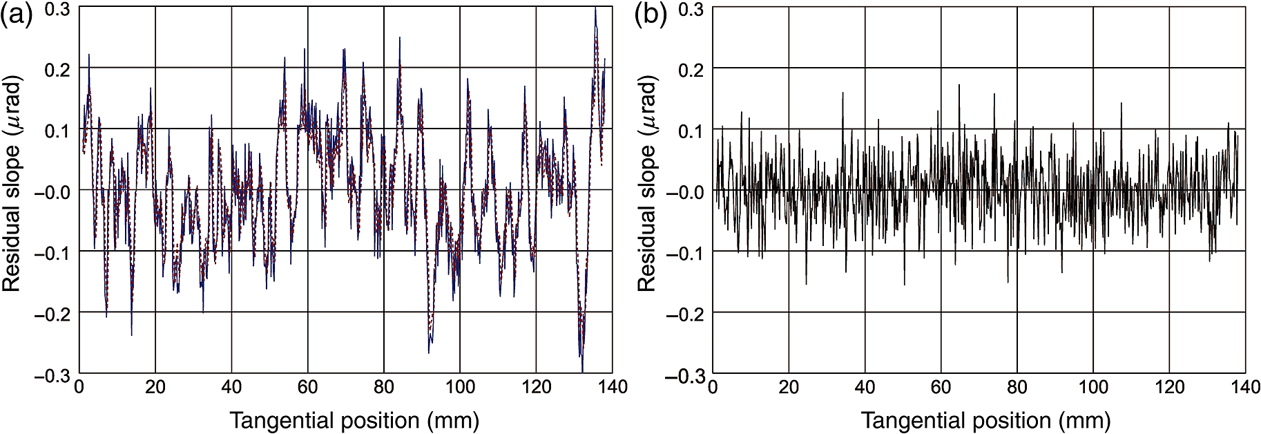$0.053 μ rad$ .

Table 1

Parameters of the ARMA model [red dashed line in Fig. 1(a)] that best fit the surface slope trace for the LCLS beam split and delay mirror measured with the ALS DLTP. In Eqs. (1)–(5), b0=1 and σ2 is equal to the standard error of the regression of 0.053 μrad (rms). The data are the regression outputs generated by EViews19 software. In the table, the standard error of the corresponding coefficient determines the statistical significance of the parameter.

Variable	Coefficient	Standard error
AR(1): $a_{1}$	0.637	0.036
AR(2): $a_{2}$	0.352	0.041
AR(5): $a_{5}$	$- 0.147$	0.027
MA(2): $b_{2}$	$- 0.0659$	0.0035

The best-fit slope trace, shown in Fig. 1(a) with the red dashed line, corresponds to the ARMA model specified in Table 1. The table, generated by EViews 8 software¹⁹ as the regression output, includes only the statistically significant ARMA parameters.

The slope difference trace shown in Fig. 1(b) is the driving noise of the ARMA model, i.e., $ν [n]$ in Eq. (1). It should be distinguished from any observation noise or measurement error. The details of the ARMA modeling of the slope metrology with the LCLS beam split and delay mirror can be found in Refs. 12 and 13.

5.2.

Autoregressive Moving Average Forecasting of Surface Topography for Mirrors with 500-mm Length, Statistically Identical to the Linac Coherent Light Source Split and Delay Mirror

The ARMA model established for the LCLS beam split and delay mirror and depicted in Table 1 was used to forecast a number of new surface slope distributions that can be thought of as the data for prospective mirrors manufactured with the same polishing process at the fabrication facility of the real mirror modeled with ARMA.

Forecasting a new slope trace with the determined ARMA model is performed in two steps. First, we generate a new sequence of white-noise-like, normally distributed residuals $ν [n]$ with a length of 500 mm (with 0.2-mm increment) corresponding to the new desired mirror length. Second, by using Eq. (1) with the ARMA parameters in Table 1 and the extended residuals, a new slope trace is generated and normalized to get the rms slope variation of $0.1 μ rad$ . Using uncorrelated sets of residuals $ν [n]$ , a number of statistically independent (inherently noncorrelating) but statistically identical (with the predetermined ARMA parameters) slope traces are generated with the EViews 8 software.¹⁹

The blue solid line in Fig. 2(a) presents one of the slope distributions, slope 09, forecast based on the described procedure and the ARMA model in Table 1. The best-fit slope trace corresponding to the ARMA model specified in Table 3 is shown in Fig. 2(a) with the red dashed line. By ARMA modeling the traces with EViews 8 in a similar manner to that described in Refs. 8 9.10.11.12.–13, we verify the statistical identity of the generated slope traces to the used ARMA model.

Fig. 2

(a) Generated slope trace slope 09 (blue solid line) and best-fit slope trace (red dashed line), corresponding to the ARMA model specified in Table 3. The rms variation of the generated slope trace is $0.101 μ rad$ . (b) Difference between the generated and fitted traces. The rms variation of the slope difference is 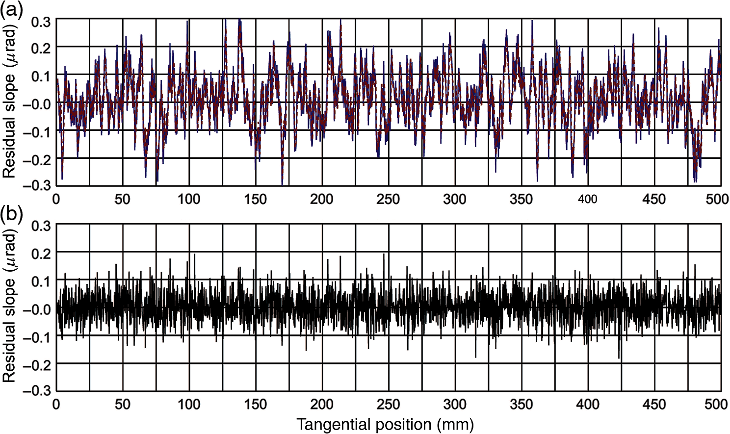$0.0523 μ rad$ .

Within statistical uncertainty, AR parameters of the ARMA models identified for the generated slope traces (see Table 2) are equal to those of the ARMA model of the measured slope trace.

Table 2

Parameters of the ARMA models that best fit the surface slope traces generated with the parent ARMA model specified in Table 1. The values of the standard error of regression are given in μrad.

Trace\parameter	AR(1): a1	AR(2): a2	AR(5): a5	MA(2): b2	Standard error of regression (μrad)
Slope 01	0.6705	0.3008	$- 0.1512$	$- 0.0041$	0.0519
Slope 02	0.6362	0.3251	$- 0.1325$	$- 0.0175$	0.0523
Slope 03	0.6032	0.3737	$- 0.1545$	$- 0.0376$	0.0541
Slope 04	0.6517	0.3208	$- 0.1447$	$- 0.0587$	0.0524
Slope 05	0.6098	0.3805	$- 0.1556$	$- 0.0950$	0.0517
Slope 06	0.6936	0.1874	$- 0.0737$	0.1624	0.0538
Slope 07	0.6166	0.4010	$- 0.1712$	$- 0.1027$	0.0531
Slope 08	0.6563	0.3244	$- 0.1349$	$- 0.0560$	0.0531
Slope 09	0.6378	0.3462	$- 0.1306$	$- 0.0419$	0.0523
Mean value	0.6418	0.3289	$- 0.1388$	$- 0.0279$	0.0527
Standard deviation	0.0296	0.0623	0.0277	0.0783	0.0008

However, the variation of the MA(2) parameter values is very large. A comparison with the results of an ARMA fit for an individual trace (e.g., slope 09 in Table 3) suggests that, in general, these ARMA fits are not sensitive to the MA term. In the case of trace slope 09, the value of $b_{2}$ is larger than its error only by a factor of 1.5. Nevertheless, the MA(2) term was kept in the parent ARMA model because it is needed to randomize the residuals of the ARMA fit for the measured slope trace in Fig. 1.

Table 3

Parameters of the ARMA model [the red dashed line in Fig. 2(a)] that best fit the generated surface slope trace slope 09. In Eqs. (1)–(5), b0=1 and σ is equal to the standard error of the regression of 0.0523 μrad (rms). Note that the ARMA fit is not sensitive to the MA term; the value of b2 is larger than its error only by a factor of 1.5. The data are the regression outputs generated by EViews19 software.

Variable	Coefficient	Standard error
AR(1): $a_{1}$	0.6378	0.0197
AR(2): $a_{2}$	0.3462	0.0284
AR(5): $a_{5}$	$- 0.1306$	0.0172
MA(2): $b_{2}$	$- 0.0419$	0.0296

The generated slope traces, such as the one shown in Fig. 2 and with the best-fit ARMA parameters in Table 2, are used to test the developed algorithm for determining the TILF weight parameters.

5.3.

AR-Time-Invariant Linear Filters with Analytically Derived Weight Coefficients for One-Dimensional Data Generated with the Known Autoregressive Moving Average Model

Here, we investigate the performance of modeling the stochastic polishing process using symmetric TILFs and the developed analytical procedure for determining the weight coefficients of the optimal filter. For this, we apply the calculation algorithm based on Eqs. (38) and (40) to fit nine slope traces generated with the known parent ARMA model as described in Secs. 5.1 and 5.2. Such generated traces are a priori the results of a uniform, stationary stochastic process; therefore, they are ideal objects for testing the developed TILF-based modeling approach.

Figure 3 illustrates the TILF approximation of the same generated trace (slope 09) as the one shown in Fig. 2 with its best ARMA fit. The blue solid line in Fig. 3 represents the generated slope trace. The optimal approximation with the developed symmetric TILF is shown in Fig. 3(a) with the red dashed line.

Fig. 3

(a) Generated slope trace slope 09 (blue solid line) and the slope trace approximation (red dashed line), obtained by application to the generated trace slope 09 of the optimal symmetric TILF with the weight coefficients in Table 3, determined using the analytical procedure presented in Sec. 4. (b) Difference between the generated and fitted traces. The rms variation of the slope difference is $0.038 μ rad$ .

For modeling, we use a symmetric TILF of order $p = 5$ , corresponding to the AR order parameter $p$ of the parent ARMA model. The question about the optimal number of coefficients is out of the scope of this present work and will be investigated elsewhere.

Table 4 presents the weight coefficients of the optimal symmetric TILF determined by application of the developed fitting procedure for nine slope traces generated with the parent ARMA model. The mean values of the coefficients estimated by averaging of nine coefficients with the same lag, as well as the standard deviations of the coefficients, are shown in the last two rows of Table 4.

Table 4

Weight coefficients of the TILF models that best fit the surface slope traces generated with the known parent ARMA model as described in Secs. 5.2 and 5.3. An extra digit in the values of the coefficients is presented to keep the data format consistent with that of the regression outputs generated by EViews19 software and shown in Tables 1–3.

Trace\coefficient	c1	c2	c3	c4	c5
Slope 01	0.3078	0.1892	0.0170	0.0753	$- 0.1009$
Slope 02	0.2812	0.2005	0.0601	0.0435	$- 0.0993$
Slope 03	0.2581	0.2124	0.0619	0.0710	$- 0.1165$
Slope 04	0.3136	0.1582	0.0322	0.0865	$- 0.1012$
Slope 05	0.2839	0.1742	0.0648	0.0673	$- 0.1019$
Slope 06	0.3137	0.1427	0.0647	0.0525	$- 0.0798$
Slope 07	0.2803	0.1711	0.0607	0.1007	$- 0.1230$
Slope 08	0.3117	0.1588	0.0486	0.0799	$- 0.1113$
Slope 09	0.2840	0.1898	0.0549	0.0510	$- 0.0886$
Mean value	0.2927	0.1774	0.0517	0.0697	$- 0.1025$
Standard deviation	0.0197	0.0224	0.0166	0.0184	0.0133

Note that if we double the mean values of the TILF weight coefficients in Table 4, they will be close to the values of the corresponding (with the same lag) AR parameters of the parent ARMA model, given in Table 1. The small difference is probably due to the extra two fitting AR-like parameters in the TILF.

One of the major advantages of the developed TILF approximation is that the residual slope, calculated as a difference between the generated slope trace and the corresponding fit, has, as predicted (see Sec. 3.2), a smaller variation than the ARMA approximation. For the slope trace slope 09, the improvement is about a factor of 1.38, close to $\sqrt{2}$ [compare Figs. 2(b) and 3(b)].

The algorithm of approximation with symmetric TILF developed in this paper is based on analytical transformation of the ACF of the stochastic process under treatment [refer to Sec. 4 and Eqs. (38) and (40)]. Therefore, in our case, it is natural to use, as a measure of fidelity of the TILF model, the difference between the ACFs of the generated trace and its TILF approximation. As a typical result, we illustrate the fidelity of the developed TILF modeling with the example of the generated trace slope 09.

Figure 4 shows the ACFs of trace slope 09 and its TILF approximation [Fig. 3(a)], as well as the difference of the ACFs. Almost over the entire range of lag values, except for a very tiny central region, the difference has a clear random character. The regions of the ACFs in the central vicinity of lag $l = 0$ are shown in Fig. 5 with enlarged scale. Here, also, there is a very close resemblance of the two ACFs, almost over the entire range of represented lags. This means that the two stochastic processes, generated and approximated, are spectrally close; therefore, the determined TILF is highly accurate.

Fig. 4

(a) ACF of the generated trace slope 09 and (b) its TILF approximation. The inset shows the difference of the ACFs in plots (a) and (b). Except for a very tiny central region, the difference has a clear random character, indicating high-accuracy of the determined TILF.

Fig. 5

(a) Central regions of the ACFs of the generated trace slope 09 (blue solid line) and its TILF approximation (red dashed line). (b) Difference between the ACFs of the generated and fitted traces in plot (a). Note that the vertical scale in (b) is increased by a factor of 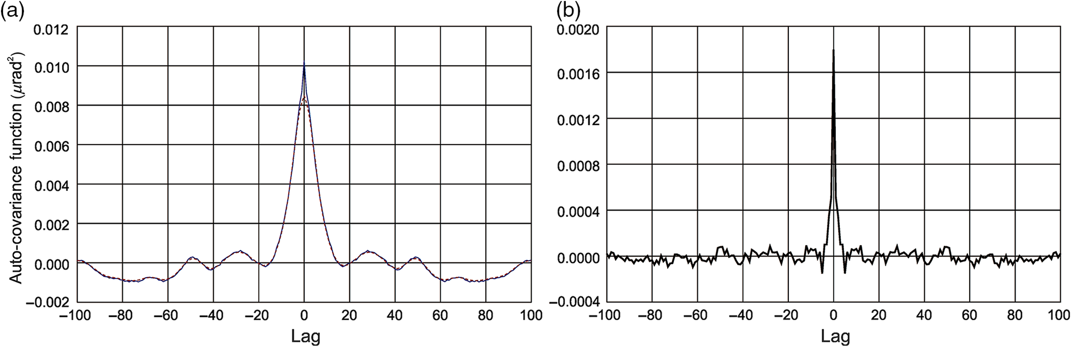$\sim 6$ .

The ACF of the residual trace [Fig. 3(b)], which is the difference between the generated trace and its TILF approximation, is shown in Fig. 6(a). The delta-function-like ACF suggests a white-noise-like character of the residual trace. For comparison, the ACF of a computer-generated white-noise trace with the same value of the rms variation is shown in Fig. 6(b). The inset in Fig. 6 represents the difference of the ACFs in Figs. 6(a) and 6(b), plotted with significantly larger scale.

Fig. 6

(a) Central regions of the ACF of the difference between the generated trace and its TILF approximation shown in Fig. 3(b). (b) ACF of white-noise trace with the same value of the rms variation. The inset shows the difference of the ACFs in plots (a) and (b). Note that the vertical scale in inset is increased by a factor of 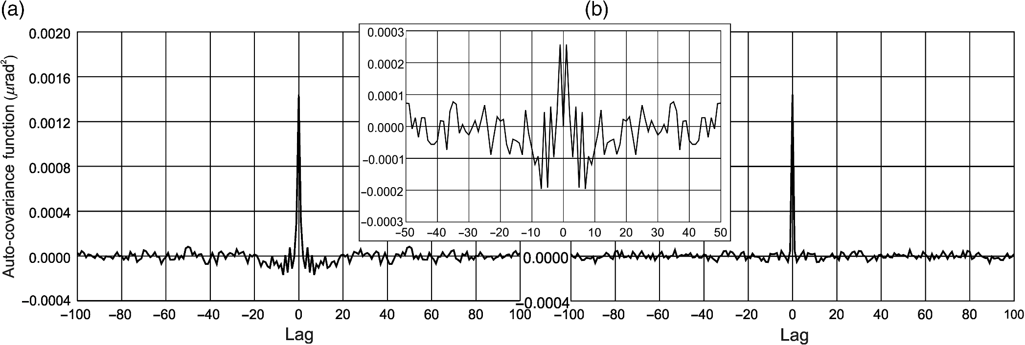$\sim 4$ .

The two-peak character of the ACF difference in Fig. 6 can be a signature of residual MA contributions to the stochastic process that are not approximated with the developed symmetric TILF model. However, ARMA modeling of the residual trace in Fig. 3(b) with EViews 8 software does not provide any reasonable model that would noticeably decrease the variance of the residual trace. This suggests an almost perfect white-noise-like distribution of the residuals.

6. Conclusion

In this work, we have continued the investigation started in Refs. 8 9.10.–11, which will potentially allow us to analytically characterize/parameterize the polishing capabilities of different vendors for x-ray optics. Based on the parametrization, the expected surface profiles of the prospective x-ray optics will be reliably simulated (forecast) prior to purchasing. The simulated surface slope and height distributions of prospective optics (before they are fabricated) can be used for estimations of the expected performance of x-ray optical systems (beamlines and x-ray telescopes).¹²^,¹³

We have analyzed a generalization of ARMA modeling with the TILF approach. We have analytically shown that the suggested symmetric TILF approximation has all the advantages of one-sided AR and ARMA modeling, along with improved fitting accuracy. It is also free of the causality problem, which can be thought of as a limitation of ARMA modeling of surface metrology data.

An algorithm for the identification of an optimal symmetric TILF with a minimum number of parameters and smallest residual error has been derived. We have verified the efficiency of the developed algorithm applied to modeling of a series of stochastic processes, which were generated with the known ARMA model determined from surface slope data of a state-of-the-art x-ray mirror.

The major application of the performed investigation of stochastic modeling of 1-D optical surface topography is in the field of x-ray reflecting optics, where the requirements for the surface quality in the direction perpendicular to the direction of the light incident at very small angle are significantly (typically by a few orders of magnitude) relaxed (see, e.g., Ref. 1 and references therein).

For more general 2-D applications, the considered TILF-based modeling of surface metrology data provides the possibility of a direct, straightforward generalization of TILF modeling to 2-D random fields. The mathematical foundations of the generalization are well established.²⁹ However, its practical realization requires the development of calculation algorithms and dedicated software for determination of the optimal TILF best-fit of measured 2-D surface slope and height distributions. The optimization can be done in a standard way, consisting of searching for the optimal filter’s weights by using, e.g., a method similar to one developed in this work. For reliable TILF forecasting of new surface topography based on measured and fitted ones, the residual noise of the fit has to have a zero-mean variance white Gaussian distribution. This is similar to the ARMA modeling; therefore, the corresponding methods and criteria could be applied to the statistical analysis of TILF modeling in dedicated software under development.

The forthcoming investigations have to solve the question about the uniqueness of the ARMA and TILF parametrizations for a certain polishing process. This can be performed, e.g., by cross-comparing the ARMA and TILF models for different optics of identical fabrication. This work is also in progress.

We did not discuss here the questions related to the application of the considered stochastic modeling to performance evaluation of particular optic and/or optical systems, or the details of forecasting surface slope topographies suitable for the simulations that also account for the detrended trend and cycles. These topics will be discussed elsewhere. Note that some related questions have been discussed in Refs. 12 and 13.

Acknowledgments

The authors are very grateful to Daniel J. Merthe, Nikolay A. Artemiev, and Daniele Cocco for their help with high-accuracy surface slope measurements of the LCLS beam split and delay mirror and to the Gary Centers and Wayne McKinney for very useful discussions. This work was supported in part by the NASA Small Business Innovation Research grant to Second Star Algonumerics, Project No. 15-1 S2.04-9193. The Advanced Light Source is supported by the Director, Office of Science, Office of Basic Energy Sciences, Material Science Division, of the U.S. Department of Energy under Contract No. DE-AC02-05CH11231 at the Lawrence Berkeley National Laboratory. This document was prepared as an account of work sponsored by the United States Government. While this document is believed to contain correct information, neither the United States Government nor any agency thereof, nor the Regents of the University of California, nor any of their employees, makes any warranty, express or implied, or assumes any legal responsibility for the accuracy, completeness, or usefulness of any information, apparatus, product, or process disclosed, or represents that its use would not infringe privately owned rights. Reference herein to any specific commercial product, process, or service by its trade name, trademark, manufacturer, or otherwise, does not necessarily constitute or imply its endorsement, recommendation, or favoring by the United States Government or any agency thereof, or the Regents of the University of California. The views and opinions of authors expressed herein do not necessarily state or reflect those of the United States Government or any agency thereof or the Regents of the University of California.

References

1.

L. Assoufid et al., “Future metrology needs for synchrotron radiation grazing-incidence optics,” Nucl. Instrum. Methods A, 467–468 267 –270 (2001). http://dx.doi.org/10.1016/S0168-9002(01)00296-0 Google Scholar

2.

K. Yamauchi et al., “Wave-optical analysis of sub-micron focusing of hard x-ray beams by reflective optics,” Proc. SPIE, 4782 271 –276 (2002). http://dx.doi.org/10.1117/12.453752 PSISDG 0277-786X Google Scholar

3.

L. Samoylova et al., “Requirements on hard x-ray grazing incidence optics for European XFEL: analysis and simulation of wavefront transformations,” Proc. SPIE, 7360 73600E (2009). http://dx.doi.org/10.1117/12.822251 PSISDG 0277-786X Google Scholar

4.

S. Moeller et al., “Photon beamlines and diagnostics at LCLS,” Nucl. Instrum. Methods A, 635 (1), S6 –S11 (2011). http://dx.doi.org/10.1016/j.nima.2010.10.125 NUIMAL 0029-554X Google Scholar

5.

M. Idir et al., “Optical and x-ray metrology,” in X-ray Optics for BES Light Source Facilities, Report of the Basic Energy Sciences Workshop on X-ray Optics for BES Light Source Facilities, 44 –55 (20132015). http://science.energy.gov/~/media/bes/pdf/reports/files/BES_XRay_Optics_rpt.pdf Google Scholar

6.

J. A. Gaskin et al., “The x-ray surveyor mission: a concept study,” Proc. SPIE, 9601 96010J (2015). http://dx.doi.org/10.1117/12.2190837 PSISDG 0277-786X Google Scholar

7.

V. V. Yashchuk et al., “Correlation analysis of surface slope metrology measurements of high quality x-ray optics,” Proc. SPIE, 8848 88480I (2013). http://dx.doi.org/10.1117/12.2024694 PSISDG 0277-786X Google Scholar

8.

Y. V. Yashchuk and V. V. Yashchuk, “Reliable before-fabrication forecasting of expected surface slope distributions for x-ray optics,” Opt. Eng., 51 (4), 046501 (2012). http://dx.doi.org/10.1117/1.OE.51.4.046501 Google Scholar

9.

Y. V. Yashchuk and V. V. Yashchuk, “Reliable before-fabrication forecasting of expected surface slope distributions for x-ray optics,” Proc. SPIE, 8141 81410N (2011). http://dx.doi.org/10.1117/12.893775 PSISDG 0277-786X Google Scholar

10.

V. V. Yashchuk, Y. N. Tyurin and A. Y. Tyurina, “Application of the time-invariant linear filter approximation to parametrization of surface metrology with high-quality x-ray optics,” Opt. Eng., 53 (8), 084102 (2014). http://dx.doi.org/10.1117/1.OE.53.8.084102 Google Scholar

11.

V. V. Yashchuk, Y. N. Tyurin and A. Y. Tyurina, “Application of time-invariant linear filter approximation to parameterization of one- and two-dimensional surface metrology with high quality x-ray optics,” Proc. SPIE, 8848 88480H (2013). http://dx.doi.org/10.1117/12.2024662 PSISDG 0277-786X Google Scholar

12.

V. V. Yashchuk, L. Samoylova and I. V. Kozhevnikov, “Specification of x-ray mirrors in terms of system performance: new twist to an old plot,” Opt. Eng., 54 (2), 025108 (2015). http://dx.doi.org/10.1117/1.OE.54.2.025108 Google Scholar

13.

V. V. Yashchuk, L. Samoylova and I. V. Kozhevnikov, “Specification of x-ray mirrors in terms of system performance: a new twist to an old plot,” Proc. SPIE, 9209 92090F (2014). http://dx.doi.org/10.1117/12.2062085 PSISDG 0277-786X Google Scholar

14.

S. M. Kay, Modern Spectral Estimation: Theory and Application, Prentice Hall, Englewood Cliffs (1988). Google Scholar

15.

G. M. Jenkins and D. G. Watts, Spectral Analysis and Its Applications, 5th ed.Emerson Adams Press, Boca Raton (2007). Google Scholar

16.

G. Rasigni et al., “Autoregressive process for characterizing statistically rough surfaces,” J. Opt. Soc. Am., A10 (6), 1257 –1262 (1993). http://dx.doi.org/10.1364/JOSAA.10.001257 JOSAAH 0030-3941 Google Scholar

17.

B.-S. Chen, B.-K. Lee and S.-C. Peng, “Maximum likelihood parameter estimation of F-ARIMA processes using the genetic algorithm in the frequency domain,” IEEE Trans. Signal Process., 50 (9), 2208 –2220 (2002). http://dx.doi.org/10.1109/TSP.2002.801918 ITPRED 1053-587X Google Scholar

18.

S. Y. Chang and H-C. Wu, “Novel fast computation algorithm of the second-order statistics for autoregressive moving-average processes,” IEEE Trans. Signal Process., 57 (2), 526 –535 (2009). http://dx.doi.org/10.1109/TSP.2008.2008234 ITPRED 1053-587X Google Scholar

19.

“EViews 8 user's guide,” www.eviews.com Google Scholar

20.

V. L. Popova and A. É. Filippov, “A model of mechanical polishing in the presence of a lubricant,” Tech. Phys. Lett., 31 (9), 788 –792 (2005). http://dx.doi.org/10.1134/1.2061748 TPLEED 1063-7850 Google Scholar

21.

S. M. Pandit, P. T. Suratkar and S. M. Wu, “Mathematical model of a ground surface profile with the grinding process as a feedback system,” Wear, 39 (2), 205 –217 (1976). http://dx.doi.org/10.1016/0043-1648(76)90049-1 WEARCJ 0043-1648 Google Scholar

22.

I. Fukumoto and T. Ayabe, “Improvement of ground surface roughness in Al-Si alloys,” Wear, 137 199 –209 (1990). http://dx.doi.org/10.1016/0043-1648(90)90136-X WEARCJ 0043-1648 Google Scholar

23.

A. Rommeveaux et al., “First report on a European round robin for slope measuring profilers,” Proc. SPIE, 5921 592101 (2005). http://dx.doi.org/10.1117/12.621087 PSISDG 0277-786X Google Scholar

24.

F. Siewert et al., “Global high-accuracy inter-comparison of slope measuring instruments,” in AIP Conf. Proc., 706 –709 (2007). http://dx.doi.org/10.1063/1.2436160 Google Scholar

25.

V. V. Yashchuk et al., “Sub-microradian surface slope metrology with the ALS developmental long trace profiler,” Nucl. Instrum. Methods A, 616 (2–3), 212 –223 (2010). http://dx.doi.org/10.1016/j.nima.2009.10.175 Google Scholar

26.

F. Siewert et al., “The nanometer optical component measuring machine: a new sub-nm topography measuring device for x-ray optics at BESSY,” in AIP Conf. Proc., 847 –850 (2004). http://dx.doi.org/10.1063/1.1757928 Google Scholar

27.

F. Siewert, H. Lammert, T. Zeschke, “The nanometer optical component measuring machine,” Modern Developments in X-Ray and Neutron Optics, 193 –200 Springer, New York (2008). Google Scholar

28.

F. Siewert, J. Buchheim and T. Zeschke, “Characterization and calibration of 2nd generation slope measuring profiler,” Nucl. Instrum. Methods A, 616 (2–3), 119 –127 (2010). http://dx.doi.org/10.1016/j.nima.2009.12.033 Google Scholar

29.

P. J. Brockwell and R. A. Davis, Time Series: Theory and Methods, 2nd ed.Springer, New York (2006). Google Scholar

30.

B. Murphy, X-Ray Split and Delay Mirrors Specifications, Menlo Park (2011). Google Scholar

31.

V. V. Yashchuk et al., “A new x-ray optics laboratory (XROL) at the ALS: mission, arrangement, metrology capabilities, performance, and future plans,” Proc. SPIE, 9206 92060I (2014). http://dx.doi.org/10.1117/12.2062042 PSISDG 0277-786X Google Scholar

32.

V. V. Yashchuk et al., “Advanced environmental control as a key component in the development of ultra-high accuracy ex situ metrology for x-ray optics,” Opt. Eng., 54 (10), 104104 (2015). http://dx.doi.org/10.1117/1.OE.54.10.104104 Google Scholar

Biography

Valeriy V. Yashchuk is currently leading the X-Ray Optics Laboratory at the Advanced Light Source, Lawrence Berkeley National Laboratory. He has authored and coauthored more than 150 scientific publications. In 1986, he was awarded the Leningrad Komsomol Prize in physics. In 2007 and 2015, he received R&D Magazine’s R&D 100 Awards for the development of laser-detected magnetic resonance imaging and binary pseudorandom calibration tool, respectively. He is an OSA fellow and a member of SPIE and APS.

Yury N. Tyurin is currently a part-time professor with the Department of Probability Theory, Faculty of Mathematics and Mechanics at Moscow State Lomonosov University, Russia. He is an author of more than 100 publications and 10 books in probability and mathematical statistics. He also enjoys developing practical applications of mathematics and statistics in industry, economics, biology, and so on, some of the developments being transferred to State Standards for Industry.

Anastasia Y. Tyurina graduated from Moscow State University as a mathematician. She is an image processing scientist and software developer. She founded a Second Star Algonumerics company in 2008. She is currently working on commercialization of her patented method of superresolution for detection of crowded point sources beyond the diffraction limit. She is consulting for governmental organizations and commercial companies, and in the course of the work, she developed a number of patented algorithms for her clients.

CC BY: © The Authors. Published by SPIE under a Creative Commons Attribution 4.0 Unported License. Distribution or reproduction of this work in whole or in part requires full attribution of the original publication, including its DOI.

Citation Download Citation

Valeriy V. Yashchuk, Yuri N. Tyurin, and Anastasia Y. Tyurina "Modeling of surface metrology of state-of-the-art x-ray mirrors as a result of stochastic polishing process," Optical Engineering 55(7), 074106 (15 July 2016). https://doi.org/10.1117/1.OE.55.7.074106

Published: 15 July 2016

Access the abstract

JOURNAL ARTICLE
11 PAGES

DOWNLOAD PAPER SAVE TO MY LIBRARY