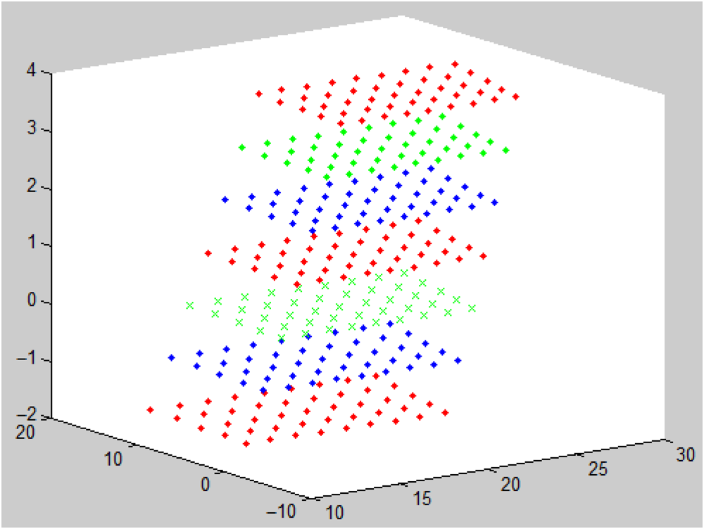
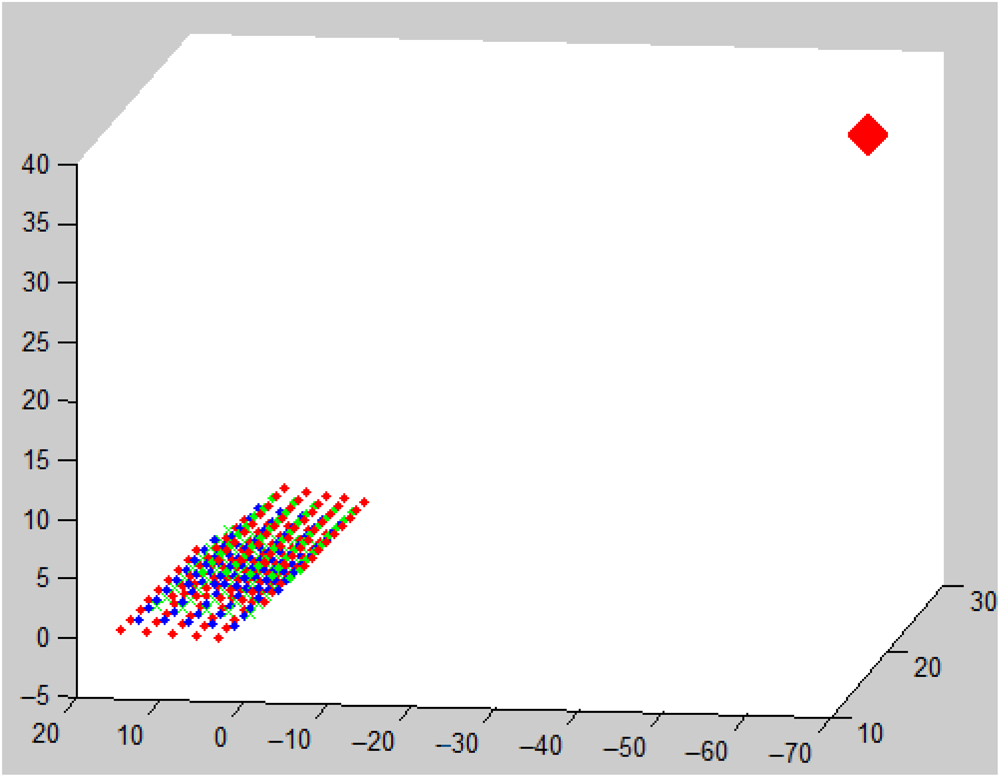
1.

Introduction

In the 16th century, the first astronomical telescope that used a refractive lens was invented by the great scientist Galileo. In 1789, Frederick William Herschel established the 1.22 m reflective telescope that uses specular mirrors. In 1948, the famous Hale telescope was established in San Diego and it used a reflective mirror with a size of 200 in. In 1976, a larger telescope with a 6-m in diameter and 25 m in length was made in Russia. Later on, more powerful telescopes with larger sizes were established, e.g., the Giant Magellan Telescope (GMT), Thirty Meter Telescope, Hubble Space Telescope, James Webb Space Telescope (JWST), and European Extremely Large Telescope (EELT), that join many small mirrors. Among them, the JWST and EELT are three-mirror anastigmatics and were built with three curved mirrors for minimum optical aberrations to achieve a wide field of view. The advantages of the three-mirror anastigmatic technique make its usage popular for military and civilian space observations. For example, the three-mirror anastigmatic Korsch telescope was used in both the Deimos-2 and DubaiSat-2 Earth observation satellites. From the above brief overview of the development history of astronomical telescopes, it can be seen that most of the designed telescopes used mirrors.

It is known that the mirrors used by the telescopes determine their imaging quality and observing ability. However, it remains a bottleneck problem to manufacture accurate enough telescope mirrors in applications where high-resolution and high-imaging quality are required for the manufactured telescopes. For instance, the accuracy of state-of-the-art optics manufacturing technology could not meet the technical requirements of the astronomical telescopes used in the projects from NASA, e.g., Astronomical Search for Origins, Structure and Evolution of the Universe, and Sun–Earth Connection). Research on new manufacturing techniques and technology in space optics is urgent and important for the development of the next generation telescopes. One important factor that reduces the imaging accuracy of the telescope is the mirror’s manufacturing errors that are defined as the differences between the practical parameters of the mirrors and their theoretical values. These parameters include the paraxial radius, geometry dimension, eccentric errors, and surface errors. To improve the manufacturing accuracy, techniques of measuring the three-dimensional (3-D) shapes of mirrors become important because the manufacturing errors of mirrors could be computed directly after their shapes are known. Although many noncontact techniques^1–10 have been developed to measure the mirrors in the past decades, none of them are capable of measuring the shapes of mirrors with adequate accuracy.

The efforts for measuring the mirror’s 3-D shape and calculating the mirror’s manufacturing errors could be traced back to the time when the telescope was invented. In 1858, Jean Foucault invented a method to measure the telescope mirrors with the knife-edge test. Unfortunately, it could only measure spherical mirrors while most telescope mirrors are aspheric instead of spherical. In addition, the Foucault method could only provide qualitative results instead of quantitative results. To yield quantitative results, it must be combined with other methods and requires great effort and considerable skills to make accurate judgments. In 1922, Vasco Ronchi invented a different technique to measure telescope mirrors and it could not provide quantitative results either. Based on the previous methods, several new methods were proposed later, e.g., the star test, the Ross null test, and the autocollimation test. However, none of them are satisfactory. In the late 1960s, the laser unequal path interferometer was invented to test spherical concave surfaces.¹¹ In the early 1970s, Karl Bath invented an interferometer to test telescope mirrors with quantitative results and it was recognized as the most informative method of that time. The Ceravolo interferometer is an alternative method with similar performances. Unfortunately, these three interferometers are only suited for testing spherical surfaces. Later on, an interferometer made by ZYGO used the peak-to-valley (PV) and root mean squares (RMS) to evaluate the quality of the mirror. However, the complexity of the optics makes PV/RMS incapable of adequately describing the mirror quality. Hence, power spectral density, slope RMS, inverse Hartmann test, and structure function (SF) are adopted widely in mirror quality evaluations.^12–18 In Ref. 16, an inverse Hartmann test was proposed for surface form measurement in the spherical coordinates with increased dynamic range and resolution. However, its accuracy was decreased compared to that in the rectangular coordinates. In Ref. 17, a tutorial about the SF analysis is presented and its advantages over Fourier-based methods were proved. In Refs. 19 and 20, researchers at the University of Arizona used the laser tracker to obtain the direct shape measurement for the GMT mirror and they achieved a measurement accuracy of $1/4\mu \mathrm{m}$. In Ref. 21, a large deformable aspherical mirror is measured with sub-$\mu \mathrm{m}$ accuracy by the software configurable optical test system. Its measurement principle is the same as that of deflectometry and it is based on the integration of the surface slope. In Ref. 22, ray tracing was used to measure the optical aberrations of aspherical lenses. All the above methods except for Ref. 22 could only indirectly give quantitative results of the surface errors for the mirror. The paraxial radius, geometry dimensions, and eccentric errors of the mirror, are outside of their capabilities.

Although Ceyhan et al.,²² claimed that their method could measure the profile of the surface, only a one-dimensional profile was given in their experiments. In Ref. 23, a method was proposed to measure the 3-D profiles of the mirrors with analytic solutions, which has the potential to achieve the zero error accuracy provided that no noise and lens distortion exist. Unfortunately, the system noise is great and the radial lens distortion of the used pico laser projector is also severe. Consequently, the measurement accuracy of Ref. 23 is limited. To improve the measurement accuracy, the pico laser projector was replaced with an silicon nitride film (SNF) laser, which is free from lens distortion and achieves better measurement accuracy.²⁴ However, the measurement accuracy is still not good enough because the noise significantly reduces the measurement accuracy. The used SNF laser does not strictly obey central projection from which some fundamental equations of the system are derived. Consequently, the reconstruction result of the system would be greatly distorted and the least deformation principle²⁴ is required to recalibrate the system, which is very time-consuming.

In this paper, a pattern modeling method is proposed to remove the noise and radial lens distortion as a whole by decreasing the degrees of freedom of the multiple laser rays to one. The proposed method registers the captured pattern with a theoretical pattern that replaces the captured pattern during the reconstruction. Since the pattern modeling method requires the projected rays to obey the principle of central projection, it could not be adopted by the system in Ref. 23 unless the SNF laser is made to be a strictly central projection. Hence, we choose the pico laser projection to generate the required laser rays in this research work. The mirror measurement system is designed according to the requirement of measuring the telescope mirrors. Due to the larger sizes of the mirrors, larger diffusive planes and a beam splitter are used with carefully selected distances. With the proposed pattern modeling method incorporated into the design system, this technique could achieve femtometer measurement accuracy (${10}^{-13}\mathrm{mm}$) for telescope mirrors, which is superior to most state-of-the-art methods.

This paper is organized as follows: Sec. 2 describes the working principle of the mirror measurement system and the method by which to calculate the projection center. In Sec. 3, noise analysis is given and the fundamental pattern modeling method is proposed. Experimental results are given in Sec. 4. Section 5 concludes the paper.

2.

System and Projection Center

The working principle of the designed system is shown in Fig. 1. Three cameras $c1$, $c2$, and $c3$ are aimed at three planes $p1$, $p2$, and $p3$, respectively. The projection center of the projector is denoted as $c$ and its symmetry point relative to the horizontal plane is $c^{\prime }$ which could be treated as the projection center of a virtual pin-hole camera. The central projection from $c^{\prime }$ intercepts the mirror plane and the diffusive plane in the same way as light goes through a pin-hole and images on the image plane. Hence, the mirror plane can be treated as the image plane of this virtual pin-hole camera. The horizontal plane $p1$ is the imaging plane of this virtual camera, it is defined as the reference plane, $z=0$ and its origin is at $o$. The laser ray is projected onto the horizontal plane $p1$ and reflected by it onto a beam splitter. The beam splitter transmits half of the ray to intercept the plane $p2$ and reflects half of the ray to intercept the plane $p3$, respectively. During the system calibration, the poses of the three cameras are estimated. The equation of the diffusive plane $p2$ or $p3$ is computed by the calibrated camera $c2$ or $c3$ and the virtual pin-hole camera. With the equation of the diffusive plane known, the homography between the camera and the diffusive plane known, and the camera coordinates of the interception points known, the 3-D world coordinate of the interception point can be computed. After the points on $p3$ are computed, they are mapped to $p4$. Thus, two points intercepting the reflected ray are obtained and this ray can be uniquely determined with a closed form solution. With the incident rays determined by the calibrated camera $c1$, the interception points of the projected pattern on the mirror surface are obtained with closed form solutions as the intersections between the incident rays and their correponding reflected rays.

Fig. 1

Working principle of the system.

A set of laser rays are projected from point $c$. The center $c$ is computed as the inception point of all the projected laser rays and it is stated as

To determine the coefficients of the incident rays, we intercept the laser rays with seven horizontal reference planes by elevating a metric lab jacks 1 mm each time. The 3-D coordinates of these intercepted points are computed by the calibrated camera $c1$ with the controlled reference planes, $z=-2$, $-1$, 0, 1, 2, 3, 4. Figure 2 shows the calculated interception points on different reference planes. With seven points known for the $i^{\prime }$th incident ray, its coefficients ${[a^i,b^i,c^i]}^{\mathrm{T}}$ are computed by singular value decomposition.

Fig. 2

Interception points of the incident rays with different horizontal reference planes.

With all the incident rays determined, we use the least square method to find the projection center $c$ whose distances to all the incident rays are the smallest. The distance of the projection center $c$ to each laser ray is calculated as

Fig. 3

Projection center denoted by the red square and its relative position to the interception points on different horizontal reference planes.

3.

Noise Analysis and Pattern Modeling

We choose the interception points on the reference plane $z=0$ and show their zoomed-in views in Fig. 4. It is seen that these five groups of points are not on straight lines as designed, which is caused by the random noise. The noise in this imaging system is mainly caused by the following two factors: (1) the captured image is affected by different influencing light sources and (2) the automatic image processing algorithms are affected by the unevenly distributed grayscales of the laser points. In addition to the noise, there are radial lens distortions that are inherent in the projectors and cameras. Both the noise and radial lens distortion greatly decrease the calibration accuracy and system measurement accuracy. Hence, they must be removed for better accuracy. For the central projection, the angle between any two projected rays does not change and all the projected rays intersect at the projection center. This is the fundamental property of the projector and camera. The proposed method is based on this property.

Fig. 4

The zoomed-in view of the interception points of the incident rays with the horizontal reference plane 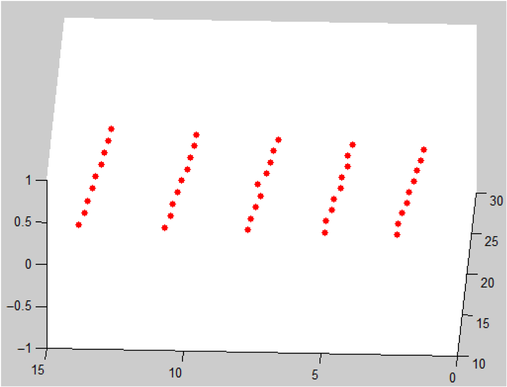$z=0$.

For two practically projected rays, the angle between them is computed by the following equation:

In the ideal pattern design coordinate system, each bright point represents one projected ray. The bright point at the center of the designed pattern corresponds to the center projected ray by the projector. The distance between two adjacent bright points is equal in both the row and column directions, which is another property that the proposed pattern modeling method relies on. We could determine the relative positions of the projected rays based on this property though their equations in the virtual coordinate system are not known. From the fundamental central projection property of the projector, we know that the angle between the center ray and any other ray is always fixed. In the ideal pattern design coordinate system, the angle between the $i$’th ray and the center ray can be computed using the following equation:

From Eq. (4), it is seen that the angle is determined by the ratio of $d_i$ and $D$, thus they are not affected by their scales. Hence, we could assume that the distance $d_i$ equals the pixel distance in the original pattern. Since the distance $D$ is unknown, we need to compute it and the following algorithm is proposed accordingly.

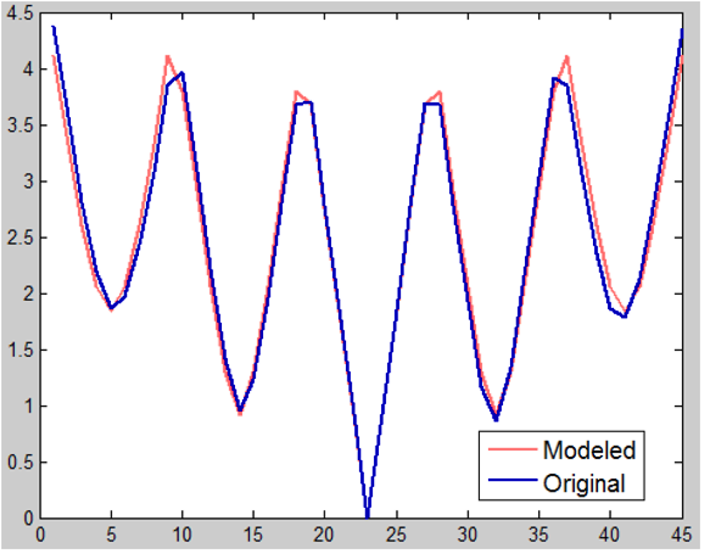
After distance $D$ is computed, the practical angle and the ideal angle between the center ray and any other ray are computed by Eqs. (3) and (4), respectively. The results are shown in Fig. 5. The practical angle computed by Eq. (3) is denoted as “original” and the ideal angle computed by Eq. (4) is denoted as “modeled.” It is seen that the angles obtained from these two different equations [Eqs. (3) and (4)] match well, but there are also obvious differences caused by the noise.

Fig. 5

Modeled angles versus original angles.

After ${\theta }_i$ is computed by Eq. (4) for each ray, the projected rays have been modeled and they are denoted as modeled rays $R_i^m$, $i=1,2,\dots .45$. To determine the interception pattern, we need to compute the plane that intercepts the projected rays. To compute the interception plane, we propose the following pattern modeling method:

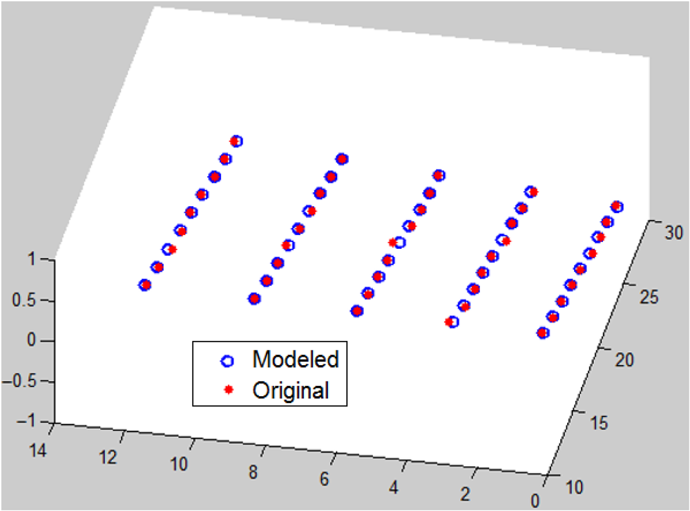
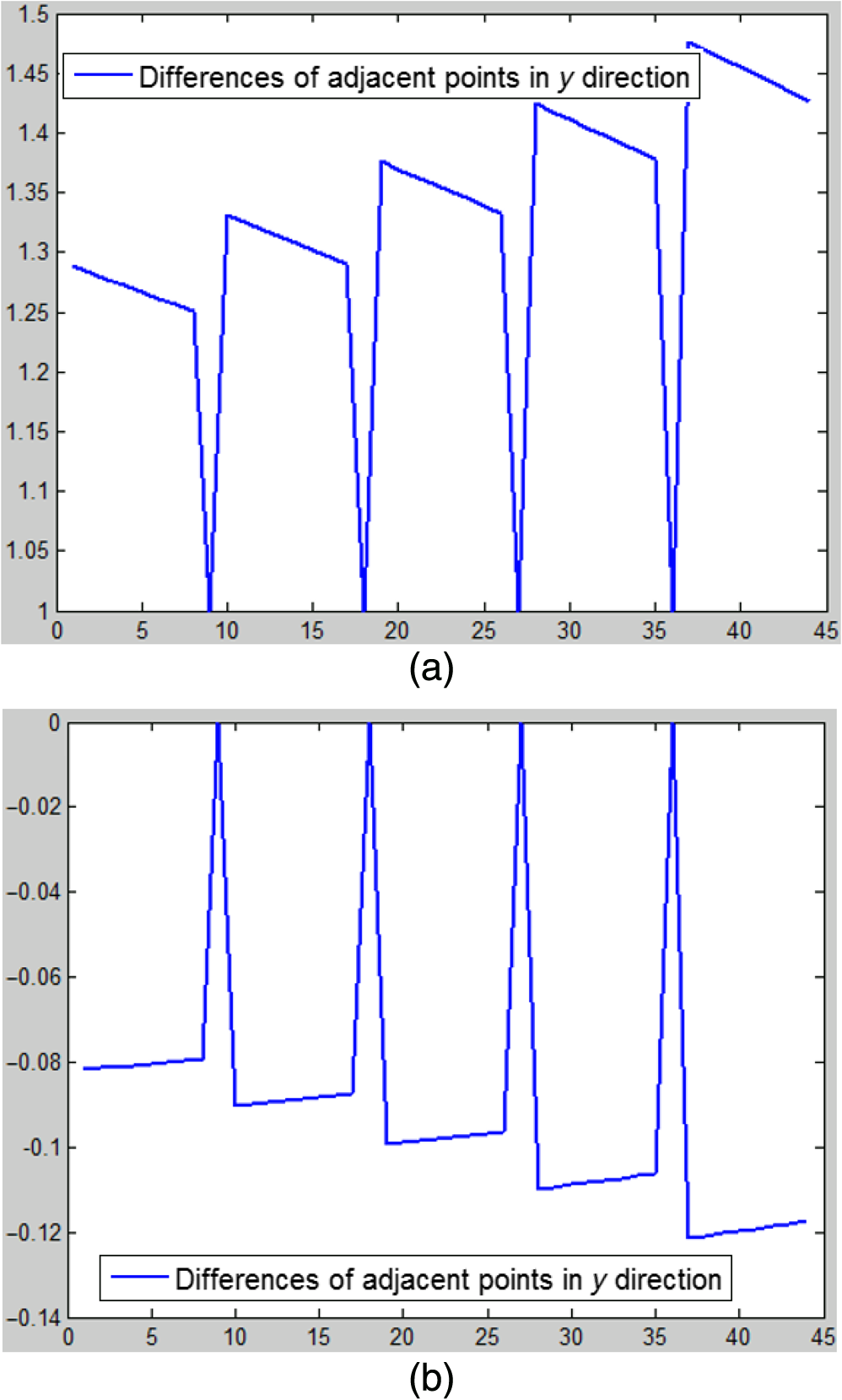
Because the intercepted points are computed in a virtual coordinate system instead of the world coordinate system, we need to convert the coordinates of the original points and the the coordinates of the modeled points by affine registration. We register the two sets of points based on the least square errors by finding the transformation matrix $A$ that makes the sum of square errors, $d_r$ minimum

Figure 6 shows the modeled points after registration (in the blue circle) versus the original points (in the red dot). It is seen that the proposed registration method performs very well. The points in each group of the modeled points are on the same straight line, which verifies that the noise and radial lens distortions were successfully removed. To see the removal effect more clearly, the differences of the $x$ and $y$ coordinates for these 45 points before pattern modeling are plotted in Figs. 7(a) and 7(b), respectively. The differences of the $x$ and $y$ coordinates for these 45 points after pattern modeling are plotted in Figs. 8(a) and 8(b), respectively. It is seen that the variation of the differences after pattern modeling becomes regular and the noise (random variation) is successfully removed. After pattern modeling, the practically captured patterns are replaced with the modeled patterns. The measurement system is calibrated with the modeled patterns as described in Ref. 20. After calibration, the mirror could be measured robustly in real time by single projection.

Fig. 6

Modeled points after registration versus original points.

Fig. 7

Differences of adjacent points before pattern modeling: (a) differences in the $x$ coordinates and (b) differences in the $y$ coordinates.

Fig. 8

Differences of adjacent points after pattern modeling: (a) differences in the $x$ coordinates and (b) differences in the $y$ coordinates.

4.

Experimental Results

Figure 9 shows the practically established system. The horizontal screen, $p1$, is placed on the top of the Metric Lab Jack whose height can be adjusted. The rays are produced by a pico laser projector and they are reflected by the mirror surface onto the beam splitter that splits the rays into two parts. Half of the rays pass through and image on the diffusive plane, $p2$. The other half of the rays are reflected and image on the diffusive plane, $p3$. The dragonfly camera $c1$ is aimed at the horizontal screen to compute the equations of the incident rays after calibration. The dragonfly cameras, $c2$ and $c3$, are aimed at the two diffusive planes, $p2$ and $p3$, respectively, and synchronically record images at $60\text{frames}/\mathrm{s}$.

Fig. 9

The developed system.

Figure 10(a) shows the designed pattern which is projected by the pico laser projector onto a horizontal diffusive plane. The brightest point in the center is the center point. The projected pattern on the horizontal screen is captured by camera $c1$ and Fig. 10(b) shows one captured example. Figures 11(a) and 11(b) show the modeled coordinates (in red) versus the original original coordinates (in blue). It is seen that the modeled coordinates and the original coordinates match well, which meets the requirement that the random variations (noise) are removed while the pattern is kept undistorted.

Fig. 10

Designed pattern and captured pattern: (a) designed pattern in the computer and (b) captured pattern by the camera.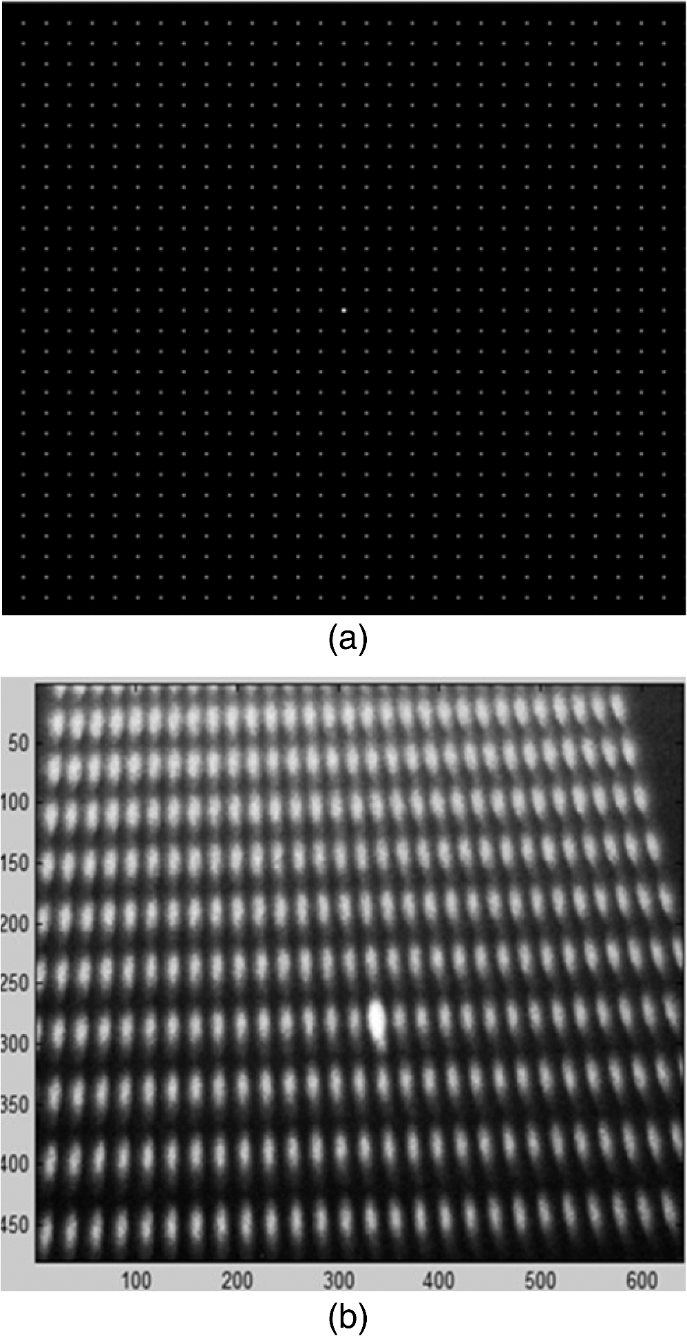

Fig. 11

Modeled coordinates versus the original coordinates: (a) $x$ coordinate and (b) $y$ coordinate.

For quantitative evaluation, we compute the RMS errors between the reconstructed points and the modeled points with the following equation:

We determine the homography between camera $c1$ and the horizontal reference plane $z=0$ using the MATLAB calibration toolbox. The determined homography could be formulated as

To quantitatively compare the measurement accuracy, we compute the RMS errors of reconstructing the flat mirror without pattern modeling first. The computed RMS error is 0.2254 mm in the $x$ coordinate, 0.1977 mm in the $y$ coordinate, and 0.0825 mm in the $z$ coordinate. The reconstructed points versus the original points are shown in Fig. 12(a), where the blue circles denote the original points and the red crosses denote the reconstructed points. We then compute the errors of reconstructing the flat mirror with pattern modeling of world coordinates in $p1$, $p2$, and $p3$. The computed RMS error is 0.0332 mm in the $x$ coordinate, 0.0278 mm in the $y$ coordinate, and 0.0113 mm in the $z$ coordinate. The reconstructed points versus the original points are shown in Fig. 12(b), where the blue circles denote the original points and the red crosses denote the reconstructed points.

Fig. 12

Illustration of the reconstruction error (a) result without modeling; (b) result with the world coordinates on the three diffusive planes modeled; and (c) result with two camera coordinates and the world coordinates on the three diffusive planes modeled.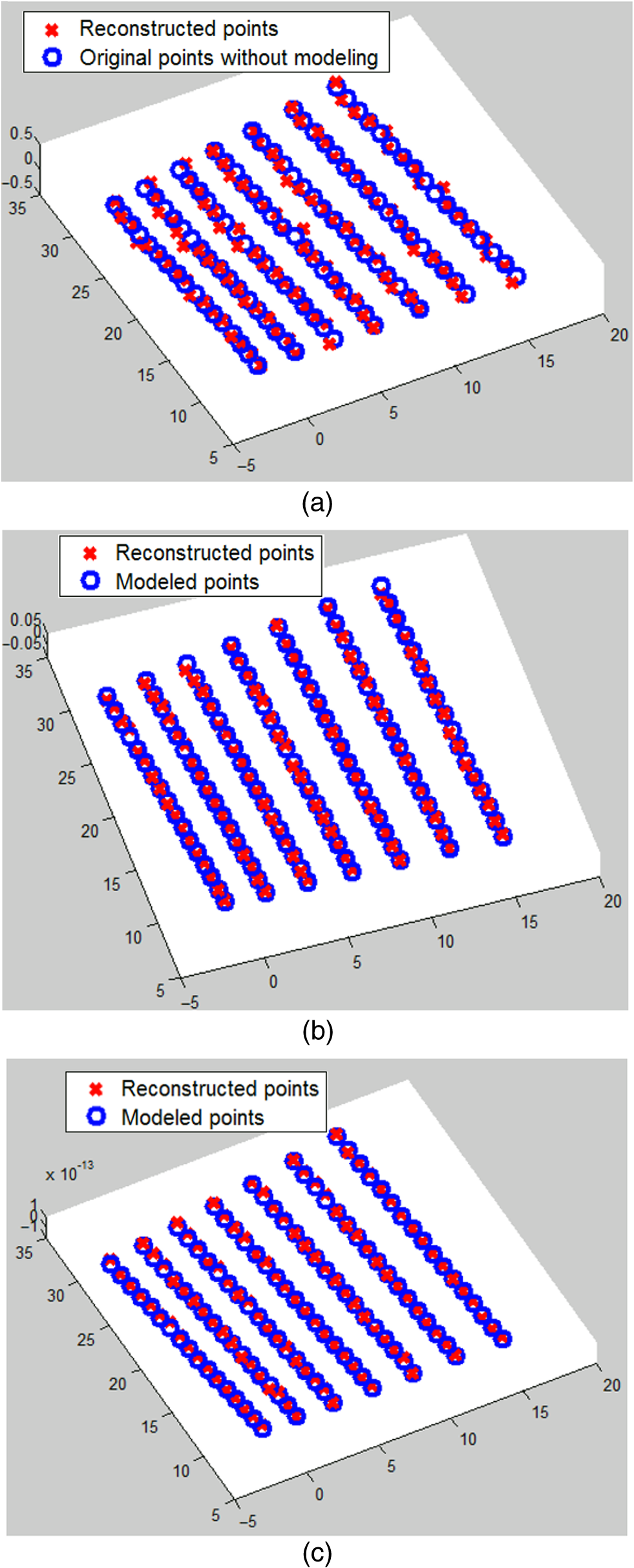

To see the pattern modeling effect further, we compute the RMS errors of reconstructing the flat mirror with pattern modeling of the camera coordinates in $c2$ and $c3$ and the world coordinates in $p1$, $p2$, and $p3$. The reconstructed points versus the original points are shown in Fig. 12(c), where the blue circles denote the original points and the red crosses denote the reconstructed points. The computed RMS error becomes $3.4681\times {10}^{-14}\mathrm{mm}$ in the $x$ coordinate, $6.6771\times {10}^{-14}\mathrm{mm}$ in the $y$ coordinate, and $2.4653\times {10}^{-14}\mathrm{mm}$ in the $z$ coordinate, respectively. At first glance, such a small RMS error seems extremely unlikely. A further thought confirms that it is reasonable. When all the involved patterns are modeled, both the calibration stage and the reconstruction stage could be assumed to be free of noise. In addition, the reconstruction error is computed between the reconstructed points and the modeled points instead of the original points. Thus, no random noise could be introduced in the evaluation stage. The reconstruction error is close to zero, but is not exactly equal zero as in our simulation with MATLAB,²³ which is caused by the use of nonideal hardware. Another adverse factor caused by the nonideal hardware is the shape distortion. Hence, the used hardware should be as precise as possible to achieve the highest measurement accuracy. Since the telescope mirrors have known forms, e.g., spherical form, plannar form, and parabolic form, we could always model the camera coordinates in $c2$ and $c3$ while measuring their shapes. Hence, the measurement accuracy of this technique for telescope mirrors is femtometers (${10}^{-13}\mathrm{mm}$). Based on theoretical analysis, this technique could achieve zero error plateau measurement accuracy when all the used devices are nearly perfect and all the involved patterns are modeled.

At last, we reconstruct a spherical convex mirror to show the strength of the proposed pattern modeling method visually. Figure 13(a) shows the reconstructed spherical convex mirror without pattern modeling. The noise severely ruined the reconstruction. Figure 13(b) shows the reconstructed spherical convex mirror with three patterns modeled. Figures 13(c) shows the reconstructed spherical convex mirror with three patterns of world coordinates and two patterns of camera coordinates modeled. It is seen that there is a noise threshold that determines if the proposed structured light technique could work effectively. Only when all the noises in the five patterns involved are eliminated will the proposed structured light technique yield satisfactory accuracy. From all these experimental results, both the strength of the proposed pattern modeling method and the proposed structured light technique were verified.

Fig. 13

Reconstruction of the convex mirror (a) result without modeling; (b) result with the world coordinates on the three diffusive planes modeled; and (c) result with two camera coordinates and the world coordinates on the three diffusive planes modeled.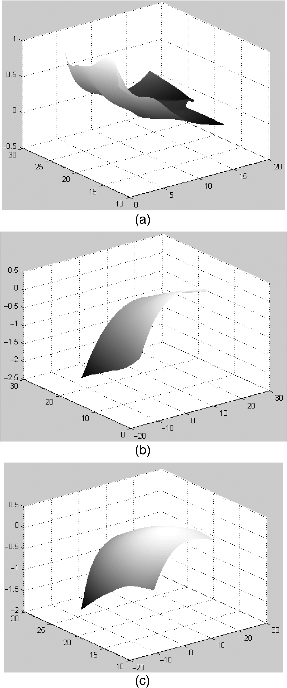

To show the superiority of this technique in measurement accuracy over state-of-the-art methods, we compared it with those state–of-the-art methods with available quantitative results and show the comparisons in Table 1. It is seen that the proposed technique is significantly more robust than state-of–the-art methods. Furthermore, some state-of-the-art methods, e.g., Ref. 21, could not measure the 3-D profiles of the mirror while this technique can. The advantage of this technique over state-of-the-art methods is further verified.

Table 1

Comparison of our method with state-of-the-art methods.

5.

Conclusion

It is important and challenging to measure the 3-D shapes of the mirrors accurately for telescope manufacturing. This paper presents a technique that is capable of robustly measuring the profiles of mirrors, which is essential for the direct measurement of manufacturing errors for the mirror. A pattern of laser rays is projected onto the mirror surface, reflected, and intercepted by two diffusive planes. With two points of the reflected ray obtained, it is uniquely determined in the world coordinate system. Further, the interception points of the projected pattern on the mirror surface are obtained by computing the intersections between the incident rays and the reflected rays. The proposed pattern modeling method is capable of removing the noise and radial lens distortion by replacing the captured pattern with a theoretical pattern that was computed by registering the captured pattern with the designed pattern. Experimental results showed that the proposed pattern modeling method could increase the measurement accuracy of this technique from 0.1 to ${10}^{-13}\mathrm{mm}$. Above all, this technique is significantly more accurate than most state-of-the-art techniques in measurement accuracy. Compared to the evaluation methods adopted by popular interferometers in mirror manufacturing, this technique is capable of measuring more mirror parameters such as the paraxial radius, geometry dimension, eccentric errors, and surface errors after the 3-D shape of the mirror is reconstructed. On the contrary, an interferometer could only evaluate the surface errors of the mirrors. Hence, this technique is promising for commercial products and devices in mirror manufacturing.