Correction of image radial distortion based on division model

Fanlu Wu; Hong Wei; Xiangjun Wang

doi:10.1117/1.OE.56.1.013108

24 January 2017 Correction of image radial distortion based on division model

Fanlu Wu, Hong Wei, Xiangjun Wang

Author Affiliations +

Optical Engineering, Vol. 56, Issue 1, 013108 (January 2017). https://doi.org/10.1117/1.OE.56.1.013108

Abstract

This paper presents an approach for estimating and then removing image radial distortion. It works on a single image and does not require a special calibration. The approach is extremely useful in many applications, particularly those where human-made environments contain abundant lines. A division model is applied, in which a straight line in the distorted image is treated as a circular arc. Levenberg–Marquardt (LM) iterative nonlinear least squares method is adopted to calculate the arc’s parameters. Then “Taubin fit” is applied to obtain the initial guess of the arc’s parameters which works as the initial input to the LM iteration. This dramatically improves the convergence rate in the LM process to obtain the required parameters for correcting image radial distortion. Hough entropy, as a measure, has achieved the quantitative evaluation of the estimated distortion based on the probability distribution in one-dimensional θ Hough space. The experimental results on both synthetic and real images have demonstrated that the proposed method can robustly estimate and then remove image radial distortion with high accuracy.

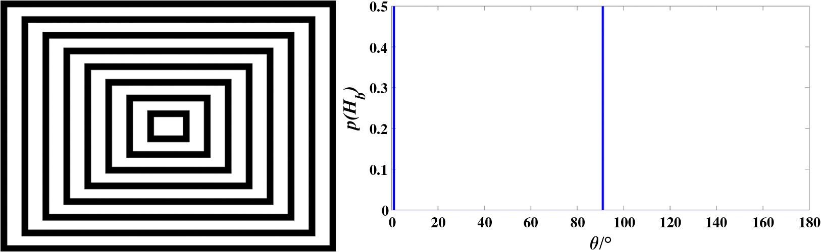
1. Introduction

Lens distortion is usually classified into three types: radial distortion, decentering distortion, and thin prism distortion.¹^–⁴ In practice, for most lenses, the radial distortion component is predominant.⁵^,⁶ It may appear as a barrel distortion or pincushion distortion. Radial distortion bends straight lines into circular arcs,⁶ violating the main invariance preserved in the pinhole camera model, in which straight lines in the world map to straight lines in the image plane.⁷ Radial distortion is the most significant type of distortion in today’s cameras.⁵^,⁸

Methods used for obtaining the parameters in the radial distortion function for correcting the distorted images can be divided roughly into two major categories: multiple views method⁹^–¹⁴ and single view method.⁶^,⁷^,¹⁵^,¹⁶ For multiple views method, the most widely used offline calibration software is the toolbox provided by Jean-Yves Bouguet.¹⁷ It can process calibration after the image is imported with a lens distortion model that includes seven parameters which are sufficient for most kinds of cameras. Although the fact that the multiple views method does not require a special condition in the scene, for example, straight lines, making it have a wide range of applications, the disadvantage of this method is that it does require multiple images which are not available in many cases, to conduct the process.⁶ In the past decades, many methods for radial distortion estimation have been proposed in research.¹⁸^–²⁶ Bukhari and Dailey²¹ proposed a method for automatic radial distortion estimation based on the plumb-line approach. They compared statistical analyses of how different circle fitting methods contribute to accurate distortion parameter estimation. They provide qualitative results on a wide variety of challenging real images. Alvarez et al.²²^,²³ proposed an algebraic approach to the estimation of the lens distortion parameters based on the rectification of lines in the image. The lens distortion parameters are obtained by minimizing a four total-degree polynomial in several variables. Lens distortion is estimated by the division model using one parameter, which allows stating the problem into the Hough transform scheme by adding a distortion parameter to better extract straight lines from the image.²⁴^–²⁶ RGB-D cameras, such as the Microsoft Kinect, have become very widely used in perceptual computing applications. To utilize the full potential of RGB-D devices, calibration must be performed to determine the intrinsic and extrinsic parameters of the color and depth sensors and to reduce lens and depth distortion. Early work for calibration of RGB-D devices includes Herrera’s method²⁷ and Smisek’s method.²⁸

In this study, our method based on the use of distorted straight lines falls in the second category. The method works on a single image in which at least three distorted straight lines exist and does not require a calibration pattern. The Brown model²⁹^–³³ is most commonly used to describe lens distortion, and it works best for lens with small distortions. However, when the distortion becomes large, it may not be satisfactory. We use Fitzgibbon’s division model⁹ of radial distortion with a single parameter. The division model is capable of expressing large distortion at a much lower order. Hartley and Kang argued that the usual assumption that the distortion center is at the image center is not safe.¹³ Our method also computes the center of radial distortion, which is important in obtaining optimal results.

The rest of this paper is structured as follows. Section 2 describes the distortion model and the estimation of distortion parameters. In Sec. 3, a detailed quantitative study is presented of the performance evaluation on both synthetic and real images. Finally, this paper comes to conclusions in Sec. 4.

2. Methodology

2.1.

Distortion Models

The Brown model that is most commonly used to describe lens distortion can be written as

Eq. (1)

{\begin{cases} x_{u} = (x_{d} - x_{0}) (1 + k_{1} r_{d}^{2} + k_{2} r_{d}^{4} + k_{3} r_{d}^{6} + \dots) + (1 + p_{3} r_{d}^{2} + \dots) {p_{1} [r_{d}^{2} + 2 (x_{d} - x_{0})^{2}] + 2 p_{2} (x_{d} - x_{0}) (y_{d} - y_{0})}, \\ y_{u} = (y_{d} - y_{0}) (1 + k_{1} r_{d}^{2} + k_{2} r_{d}^{4} + k_{3} r_{d}^{6} + \dots) + (1 + p_{3} r_{d}^{2} + \dots) {p_{2} [r_{d}^{2} + 2 (y_{d} - y_{0})^{2}] + 2 p_{1} (x_{d} - x_{0}) (y_{d} - y_{0})}, \end{cases}

where

(x_{u}, y_{u})

and

(x_{d}, y_{d})

are the corresponding coordinates of an undistorted point and a distorted point in an image, respectively.

r_{d} = \sqrt{{(x_{d} - x_{0})}^{2} + {(y_{d} - y_{0})}^{2}}

is the Euclidean distance of the distorted point to the distortion center

(x_{0}, y_{0})

.

According to Zhang,⁵ the radial distortion is predominant. The most commonly used radial distortion model can be written as

Eq. (2)

{\begin{cases} x_{u} = x_{d} (1 + λ_{1} r_{d}^{2} + λ_{2} r_{d}^{4} + \dots), \\ y_{u} = y_{d} (1 + λ_{1} r_{d}^{2} + λ_{2} r_{d}^{4} + \dots), \end{cases}

supposing that the distorted center

(x_{0}, y_{0})

is the center of the image. This model works best for lenses with small distortions. However, when the distortion becomes large, it may not be satisfactory and many other factors have to be taken into account in practice.⁶

Fitzgibbon⁹ proposed the division model as

Eq. (3)

{\begin{cases} x_{u} = \frac{x_{d}}{1 + λ_{1} r_{d}^{2} + λ_{2} r_{d}^{4} + \dots}, \\ y_{u} = \frac{y_{d}}{1 + λ_{1} r_{d}^{2} + λ_{2} r_{d}^{4} + \dots} . \end{cases}

The most remarkable advantage of the division model over the Brown model is that it is able to express a large distortion at a much lower order. In particular, for many cameras, a single parameter would suffice.⁹^,¹⁰ In our study, we use the single parameter division model

Eq. (4)

{\begin{cases} x_{u} = \frac{x_{d}}{1 + λ r_{d}^{2}}, \\ y_{u} = \frac{y_{d}}{1 + λ r_{d}^{2}} . \end{cases}

2.2.

Distortion of a Straight Line

Under the single parameter division model, the distorted image of a straight line can be treated as a circular arc.⁶ The equation of a straight line is expressed as

Eq. (5)

A x_{u} + B y_{u} + C = 0 .

From Eq. (4), we have

Eq. (6)

A \frac{x_{d}}{1 + λ r_{d}^{2}} + B \frac{y_{d}}{1 + λ r_{d}^{2}} + C = 0,

then, we obtain a circle equation

Eq. (7)

x_{d}^{2} + y_{d}^{2} + \frac{A}{C λ} x_{d} + \frac{B}{C λ} y_{d} + \frac{1}{λ} = 0 .

If $(x_{0}, y_{0})$ is the center of radial distortion, we have

Eq. (8)

{(x_{d} - x_{0})}^{2} + {(y_{d} - y_{0})}^{2} + \frac{A}{C λ} (x_{d} - x_{0}) + \frac{B}{C λ} (y_{d} - y_{0}) + \frac{1}{λ} = 0 .

Let $D = \frac{A}{C λ} - 2 x_{0}$ , $E = \frac{B}{C λ} - 2 y_{0}$ , $F = x_{0}^{2} + y_{0}^{2} - \frac{A}{C λ} x_{0} - \frac{B}{C λ} y_{0} + \frac{1}{λ}$ , then, we have

Eq. (9)

x_{d}^{2} + y_{d}^{2} + D x_{d} + E y_{d} + F = 0,

and

Eq. (10)

x_{0}^{2} + y_{0}^{2} + D x_{0} + E y_{0} + F - \frac{1}{λ} = 0 .

Equation (9) indicates that a group of parameters

(D, E, F)

can be determined by fitting a circle to an arc which is extracted from the image. The circular arc in the image is projected from a straight line in the world. By extracting at least three arcs and determining three groups of parameters

(D, E, F)

, the distortion center can be estimated by solving the linear equations of

Eq. (11)

{\begin{cases} (D_{1} - D_{2}) x_{0} + (E_{1} - E_{2}) y_{0} + (F_{1} - F_{2}) = 0, \\ (D_{1} - D_{3}) x_{0} + (E_{1} - E_{3}) y_{0} + (F_{1} - F_{3}) = 0, \end{cases}

and an estimate of

λ

can be obtained from

Eq. (12)

λ = \frac{1}{x_{0}^{2} + y_{0}^{2} + D x_{0} + E y_{0} + F} .

When extracting more than three arcs from an image and determining these parameters

(D, E, F)

, the parameter

(x_{0}, y_{0}, λ)

can be obtained based on the Levenberg–Marquardt (LM) scheme. Although the method requires at least three distorted lines residing in an image, it can cope with a situation in which fewer lines are found by adding more images taken by the same camera with different capturing angles. As long as there is a line involved in the scene, the method is applicable.

2.3.

Method of Circle Fitting

To find arcs, we first extract edges using the Canny operator. Then we track all the edge points associated with a starting point. From a given starting point, we track in one direction, storing the coordinates of the edge points in an array and label the pixels in the edge image. When no more connected points are found, we return to the start point and track in the opposite direction. Finally, a check for the overall number of edge points found is made and the edge is ignored if it is too short.

After the initial arc identification process, an initial guess of parameters is assigned to each resulting arc, followed by the LM iterative nonlinear least squares method to produce the optimized parameters. Taubin fit is used for the initial guess.³⁴ It uses four parameters to specify a circle: $a (x^{2} + y^{2}) + b x + c y + d = 0$ , with $a \neq 0$ . The center of the circle is $(\frac{- b}{2 a}, \frac{- c}{2 a})$ and the radius is given by $r = \sqrt{{(\frac{- b}{2 a})}^{2} + {(\frac{- c}{2 a})}^{2} - \frac{d}{a}}$ . It minimizes the objective function $Ω (a, b, c, d) = \sum_{i = 1}^{N} (a x_{i}^{2} + a y_{i}^{2} + b x_{i} + c y_{i} + d^{2})$ , subject to the constraint that $4 a^{2} \overline{z} + 4 a b \overline{x} + 4 a c \overline{y} + b^{2} + c^{2} = 1$ , where $\bar{x}$ is the mean of the points’ $x$ coordinates, $\overline{y}$ is the mean of the points’ $y$ coordinates, and $\bar{z} = \frac{1}{N} Σ_{i = 1}^{N} (x_{i}^{2} + y_{i}^{2})$ . The objective function for LM fit³⁵ is $Ω (x_{c}, y_{c}, r) = \sum_{i = 1}^{N} {(r_{i} - r)}^{2}$ , where $r_{i} = \sqrt{{(x_{i} - x_{c})}^{2} + {(y_{i} - y_{c})}^{2}}$ .

3. Result and Discussion

Experiments were carried out on both synthetic and real image data. The performance evaluation of the proposed approach was conducted. We use Hough entropy to evaluate the quality of recovering distorted synthetic images. The Hough transform is a technique that can find lines in images.³⁶ The basis of the technique is the transform of a line to a point in a Hough space. A line is represented by a single point in the two-dimensional (2-D) Hough space of $ρ \times θ$ , in which the values of these points vary. In our case, a specified threshold is set empirically as $0.3 * \max$ (Hough space) to obtain all peaks which represents lines. A straight line in the distorted image is treated as a circular arc and we only use the values of $θ$ to measure the straightness. So transform the 2-D Hough space of $ρ \times θ$ to a one-dimensional (1-D) $θ$ space by summing over the $ρ$ values for each $θ$ , then the Hough entropy is defined as

Eq. (13)

H = - \sum_{b = 1}^{Bins} p (H_{b}) \log_{2} [p (H_{b})],

where Bins is the number of

θ

discrete bins (we set

Bins = 180

), and

p (H_{b})

is the value of probability.

3.1.

Tests on Synthetic Images

An image in size of $640 \times 480 pixels$ , as shown in Fig. 1, was used as a source image ( $H = 1$ ). Synthetic images are generated from the source image with given information of the distortion parameters $(x_{0}, y_{0}, λ)$ . We performed three series of experiments with synthetic images.

Fig. 1

Source image and the corresponding 1-D Hough transforms.

3.1.1.

Varying $λ$

In the first series, synthetic images are obtained with distortion parameters $(320,240, λ)$ , with varying $λ$ at different levels (from extreme pincushion to barrel distortion). For a positive $λ$ (pincushion distortion), the size of synthetic images is larger than $640 \times 480$ pixels, and the distortion center is different from known parameters of $(x_{0}, y_{0}, λ)$ . For a negative $λ$ (barrel distortion), the size of synthetic images is $640 \times 480 pixels$ , and the distortion center is fixed at (320, 240). The synthetic images, corrected images, and the corresponding 1-D Hough transforms are shown in Fig. 2. For the extreme case of $λ \geq 5.0 \times 10^{- 6}$ , we only map the points for which $r_{d}^{2} \leq 1 / (4 λ)$ , resulting in a circular valid region around the image center.

Fig. 2

Correction of synthetic images (with different $λ$ ). (a) For positive $λ$ . First column: distorted images at different levels of $λ$ . Second column: corresponding 1-D Hough transforms of first column. Third column: corrected images of first column. Fourth column: corresponding 1-D Hough transforms of third column. (b) For negative $λ$ . First column: distorted images at different levels of $λ$ . Second column: corresponding 1-D Hough transforms of first column. Third column: corrected images of first column. Fourth column: corresponding 1-D Hough transforms of third column.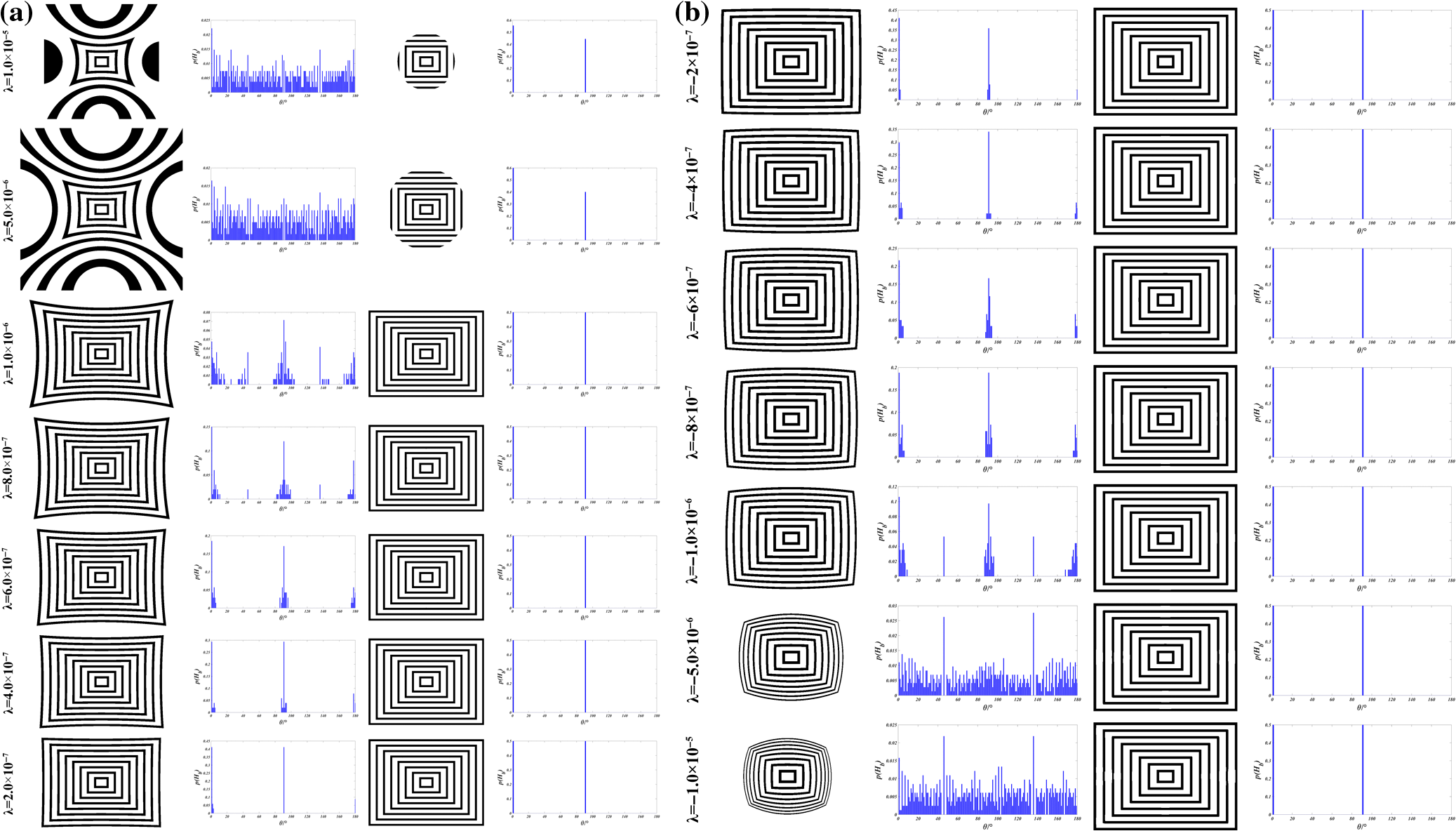

As shown in Fig. 2, the proposed method works very well for all distortion parameters in the test interval and remove image radial distortion with high accuracy. Estimated results of distortion parameters and Hough entropy of corrected images are shown in Table 1. The initial estimation only extracts three arcs which have maximum distortion, and the estimation based on the LM method extracts sixteen arcs which also have maximum distortion. Dis is the Euclidean distance between $(x_{0}, y_{0})_{true}$ and $(x_{0}, y_{0})_{estimate}$ . Rel is the relative error for $λ$ , i.e., $| (λ_{estimate} - λ_{true}) / λ_{true} |$ . Dis, $λ_{estimate}$ , and Rel can be found in Table 1.

Table 1

Estimated results of the synthetic images from Fig. 2.

λtrue	Initial estimate			Estimate by LM method			H
λtrue	λestimate	Rel	Dis	λestimate	Rel	Dis	H
$1.0 \times 10^{- 5}$	$0.999777183 \times 10^{- 5}$	$2.2817 \times 10^{- 4}$	0.6704	$0.99993718 \times 10^{- 5}$	$6.282 \times 10^{- 5}$	0.7208	0.9911
$5.0 \times 10^{- 6}$	$5.0006619 \times 10^{- 6}$	$1.3237 \times 10^{- 4}$	0.7185	$5.0002084 \times 10^{- 6}$	$4.169 \times 10^{- 5}$	0.7043	0.9710
$1.0 \times 10^{- 6}$	$1.0007869 \times 10^{- 6}$	$7.8688 \times 10^{- 4}$	0.6429	$0.9996487 \times 10^{- 6}$	$3.5131 \times 10^{- 4}$	1.1189	1
$8.0 \times 10^{- 7}$	$7.978815 \times 10^{- 7}$	$2.64816 \times 10^{- 3}$	0.9011	$8.002692 \times 10^{- 7}$	$3.3644 \times 10^{- 4}$	0.9705	1
$6.0 \times 10^{- 7}$	$6.007668 \times 10^{- 7}$	$1.27806 \times 10^{- 3}$	1.4614	$6.002536 \times 10^{- 7}$	$4.2261 \times 10^{- 4}$	0.6508	1
$4.0 \times 10^{- 7}$	$4.025900 \times 10^{- 7}$	$6.47499 \times 10^{- 3}$	4.2259	$3.999954 \times 10^{- 7}$	$1.146 \times 10^{- 5}$	3.0141	1
$2.0 \times 10^{- 7}$	$2.068505 \times 10^{- 7}$	$3.425237 \times 10^{- 2}$	3.9462	$1.995506 \times 10^{- 7}$	$2.24694 \times 10^{- 3}$	6.4786	1
$- 2.0 \times 10^{- 7}$	$- 2.056167 \times 10^{- 7}$	$2.808350 \times 10^{- 2}$	11.7907	$- 2.011946 \times 10^{- 7}$	$5.97300 \times 10^{- 3}$	7.3833	1
$- 4.0 \times 10^{- 7}$	$- 3.951756 \times 10^{- 7}$	$1.206111 \times 10^{- 2}$	6.5535	$- 3.966594 \times 10^{- 7}$	$8.35147 \times 10^{- 3}$	1.9250	1
$- 6.0 \times 10^{- 7}$	$- 6.062686 \times 10^{- 7}$	$1.044762 \times 10^{- 2}$	3.8644	$- 6.025610 \times 10^{- 7}$	$4.26833 \times 10^{- 3}$	1.6750	1
$- 8.0 \times 10^{- 7}$	$- 7.919760 \times 10^{- 7}$	$1.003003 \times 10^{- 2}$	3.4495	$- 8.008144 \times 10^{- 7}$	$1.01804 \times 10^{- 3}$	1.1657	1
$- 1.0 \times 10^{- 6}$	$- 1.0014953 \times 10^{- 6}$	$1.49534 \times 10^{- 3}$	0.8899	$- 0.9995671 \times 10^{- 6}$	$4.3291 \times 10^{- 4}$	0.7946	1
$- 5.0 \times 10^{- 6}$	$- 4.9972071 \times 10^{- 6}$	$5.5859 \times 10^{- 4}$	1.0859	$- 5.0008469 \times 10^{- 6}$	$1.6937 \times 10^{- 4}$	0.9439	1
$- 1.0 \times 10^{- 5}$	$- 0.99546012 \times 10^{- 5}$	$4.53988 \times 10^{- 3}$	0.3783	$- 1.00022696 \times 10^{- 5}$	$2.2696 \times 10^{- 4}$	0.5654	1

From Table 1, we can see that the proposed approach produces convincing distortion parameters which are very close to the true distortion parameters used for generating the synthetic images. This method is very robust even at extreme cases. Table 1 also shows that the LM method provides better estimates than the three arcs methods. Although the LM method may slightly increase Dis, it has dramatically reduced Rel. The results in terms of relative estimation error for $λ$ in Table 1 show quite clearly that our method is extremely accurate at estimating $λ$ , the estimated results of Rel based on the LM method at the range of $10^{- 3}$ to $10^{- 5}$ . Rel increases when $λ$ is close to zero, which reflects the following factor: since the true value is extremely small, small deviations between the estimated and true parameter values give relatively large errors. Table 1 shows quite clearly that the estimated results of Dis based on the LM method are less than 8 pixels. Furthermore in the case of $| λ | \geq 6.0 \times 10^{- 7}$ , Dis are less than 2 pixels. Hough entropy is always equal to 1 except for the extreme case of $λ \geq 5.0 \times 10^{- 6}$ . For this case, we only map the points for which $r_{d}^{2} \leq 1 / (4 λ)$ [see Fig. 2(a)]. $θ$ is always equal to 0 (or 90) in the Hough space even for the extreme case of $λ \geq 5.0 \times 10^{- 6}$ , which shows that our method is robust. Real images may not contain too many distorted straight line. Fortunately, the results in Table 1 show quite clearly that the initial estimation only extracting three arcs which have satisfactory accuracy.

3.1.2.

Varying distortion center

In the second series, synthetic images are obtained with the distortion fixed at a moderate level of barrel distortion $(λ = - 1.0 \times^{- 6})$ while varying the distortion center. The synthetic images, corrected images, and the corresponding 1-D Hough transforms are presented in Fig. 3. Dis, $λ_{estimate}$ , and Rel can be found in Table 2.

Fig. 3

Correction of synthetic images (with different distortion center). First column: distorted images. Second column: corresponding 1-D Hough transforms of first column. Third column: corrected images of first column. Fourth column: corresponding 1-D Hough transforms of third column.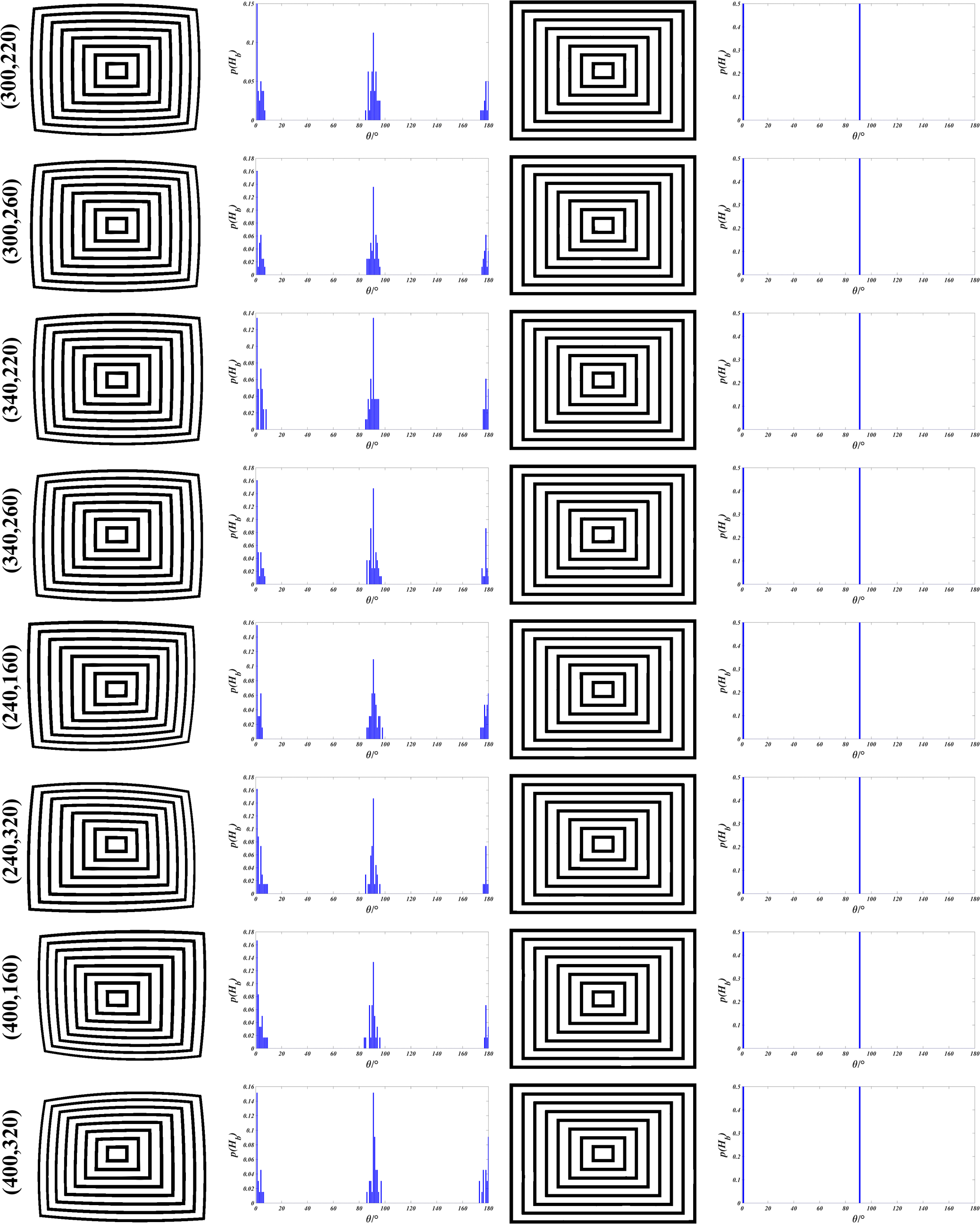

Table 2

Estimated results of the synthetic images from Fig. 3.

(x0,y0)true	Initial estimate				Estimate by LM method				H
(x0,y0)true	λestimate	Rel	(x0,y0)estimate	Dis	λestimate	Rel	(x0,y0)estimate	Dis	H
(300, 220)	$- 0.9993661 \times 10^{- 6}$	$6.3387 \times 10^{- 4}$	(302.0406, 220.5043)	2.1019	$- 0.9997905 \times 10^{- 6}$	$2.0946 \times 10^{- 4}$	(301.1228, 219.5050)	1.2271	1
(300, 260)	$- 0.9997047 \times 10^{- 6}$	$2.9529 \times 10^{- 4}$	(301.7350, 259.7820)	1.7486	$- 1.0000697 \times 10^{- 6}$	$6.974 \times 10^{- 5}$	(300.9076, 259.0131)	1.3408	1
(340, 220)	$- 1.0040027 \times 10^{- 6}$	$4.00267 \times 10^{- 3}$	(337.1097, 219.6016)	2.9176	$- 1.0002655 \times 10^{- 6}$	$2.6555 \times 10^{- 4}$	(338.4051, 219.1870)	1.7902	1
(340, 260)	$- 1.0036289 \times 10^{- 6}$	$3.62891 \times 10^{- 3}$	(337.0461, 258.7703)	3.1997	$- 0.9997154 \times 10^{- 6}$	$2.8457 \times 10^{- 4}$	(337.7498, 259.1804)	2.3948	1
(240, 160)	$- 1.0012700 \times 10^{- 6}$	$1.27000 \times 10^{- 3}$	(239.0277, 159.8959)	0.9778	$- 0.9996601 \times 10^{- 6}$	$3.3993 \times 10^{- 4}$	(237.9878, 158.7605)	2.3633	1
(240, 320)	$- 0.9969717 \times 10^{- 6}$	$3.02829 \times 10^{- 3}$	(239.9595, 319.4118)	0.5896	$- 1.0000098 \times 10^{- 6}$	$9.84 \times 10^{- 6}$	(238.2006, 320.1384)	1.8048	1
(400, 160)	$- 1.0028122 \times 10^{- 6}$	$2.81218 \times 10^{- 3}$	(399.3107, 159.8861)	0.6987	$- 0.9998814 \times 10^{- 6}$	$1.1862 \times 10^{- 4}$	(398.1673, 159.2641)	1.9749	1
(400, 320)	$- 1.0023331 \times 10^{- 6}$	$2.33315 \times 10^{- 3}$	(398.8879, 317.7069)	2.5486	$- 1.0000925 \times 10^{- 6}$	$9.248 \times 10^{- 5}$	(398.1597, 319.5542)	1.8935	1

As shown in Fig. 3, the proposed method works very well for all distortion parameters in the test interval and removes image radial distortion with high accuracy. From Table 2, we can see that our method gives good results about the distortion parameter $(x_{0}, y_{0}, λ)$ . The results in terms of relative estimation error for $λ$ in Table 2 show quite clearly that our method is extremely accurate at estimating $λ$ , and for estimated results of Rel based on the LM method at the range of $10^{- 4}$ to $10^{- 6}$ . The estimated results of Dis based on the LM method are less than 3 pixels. Hough entropy is always equal to 1, which shows that our method is robust.

3.1.3.

Comparison to another technique

To gauge the accuracy of our method, we have compared it to the method developed by Alvarez et al.²²^,²³ Alvarez et al. have deployed a demo web site³⁷ for their method that allows users to submit an image for removing distortion after manually selecting distorted lines from it. For a fair comparison, the same three lines were used in both Alvarez’s method and our method. A synthetic image was generated from the source image with given information of distortion parameters $(320,240, λ = - 1.0 \times 10^{- 6})$ . The synthetic image, corrected images, and the corresponding 1-D Hough transforms are presented in Fig. 4. Dis, $(x_{0}, y_{0})_{estimate}$ , and $H$ can be found in Table 3. Compared to the source image (Fig. 1), the content of the corrected image [Fig. 4(b)] which generated from Alvarez’s method is zoomed out, and content of the corrected image [Fig. 4(c)] which is generated from the proposed method is unchanged. As shown in Fig. 4, the proposed method outperforms Alvarez’s method in terms of visual qualities. From Table 3, we can see quantitatively that the proposed method has dramatically reduced Dis, and the Hough entropy is equal to the source image. Moreover, compared to Alvarez’s method which requires manual intervention to select distorted straight lines, the proposed method requires much less processing time.

Fig. 4

(a) Synthetic image and corresponding 1-D Hough transforms. (b) Corrected image of (a) which generated from Alvarez’s method and corresponding 1-D Hough transforms. (c) Corrected image of (a) which generated from the proposed method and corresponding 1-D Hough transforms.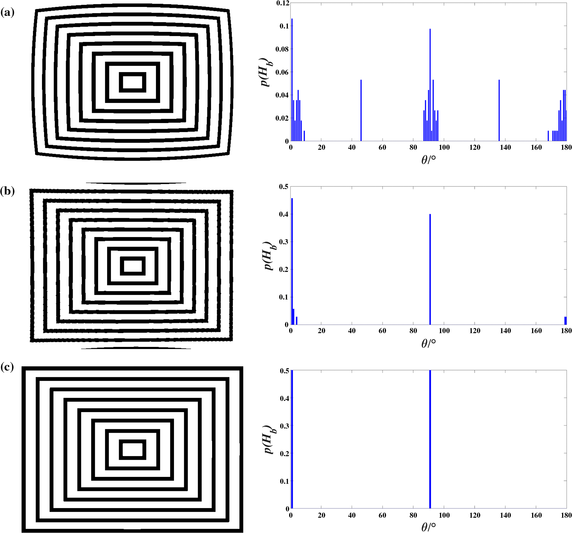

Table 3

Results comparison of the synthetic image from Fig. 4.

Algorithm	(x0,y0)estimate	Dis	H
Alvarez et al.	(330.0076, 235.0030)	11.1858	1.7206
Proposed	(319.6754, 239.1714)	0.8899	1

3.2.

Tests on Real Images

The original tested real images and corrected images are shown in Fig. 5, the original image of (a)–(g) are obtained from the Image Processing on Line website.³⁸ From Fig. 5, we can obviously observe the distortion (left in a pair) as well as correction (right in a pair). These results demonstrated that the radial distortion has been successfully removed in the recovered images. It shows the robustness and accuracy of the proposed approach in the radial distortion correction.

Fig. 5

Correction of real images. Some lines that are straight in the world have been annotated with red straight lines in the corrected image, showing strong vanishing points. (a) (b) (c) (d) (g) are building, (e) bedroom, (f) solar power plant, and (h) the ceiling of corridor.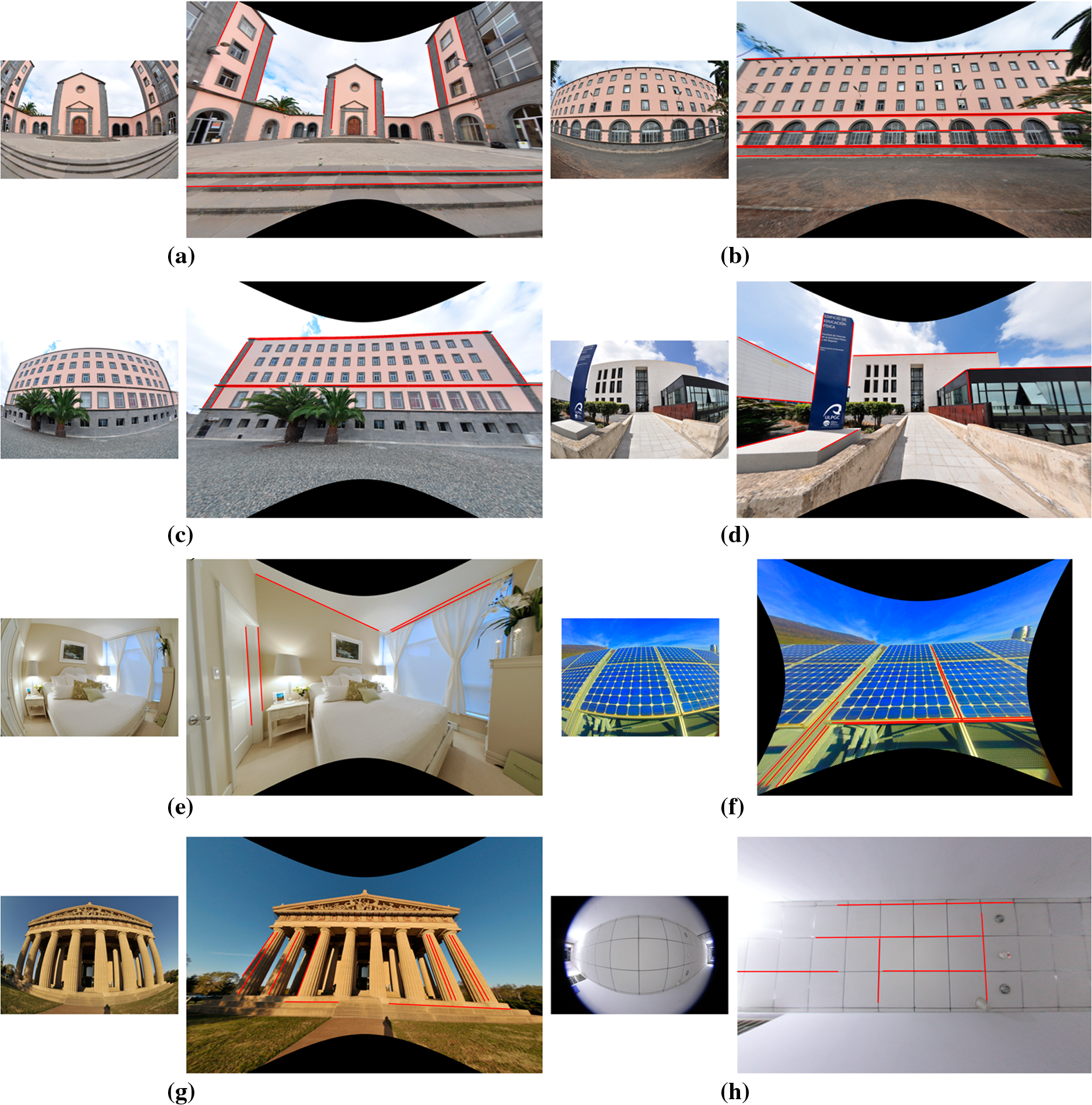

For the quantitative evaluation, we have compared the proposed method to Zhang’s method⁵ and Alvarez’s method. For Zhang’s method, it has to use a calibration pattern (checkerboard with black-and-white squares) to estimate the camera’s intrinsic parameters, therefore, its process takes a much longer time. For the comparison of Alvarez’s method and the proposed method, the same three distorted lines were taken for the purpose. The real image, corrected images, and the corresponding 1-D Hough transforms are presented in Fig. 6. As expected, the proposed method outperforms Zhang’s method and Alvarez’s method in terms of visual qualities. Compared to Zhang’s method which involves camera calibration and Alvarez’s method which requires manual intervention to select distorted straight lines, the proposed method is much faster in terms of processing time. The probability distribution in 1-D $θ$ Hough space in Fig. 6(d) shows that our method is much more uniform at 0 deg and 180 deg compared to those in Figs. 6(b) and 6(c). This means that the proposed method has a more satisfactory result in removing image radial distortion.

Fig. 6

(a) Real image and corresponding 1-D Hough transforms. (b) Corrected image of (a) which generated from Zhang’s method and corresponding 1-D Hough transforms. (c) Corrected image of (a) which generated from Alvarez’s method and corresponding 1-D Hough transforms. (d) Corrected image of (a) which generated from the proposed method and corresponding 1-D Hough transforms.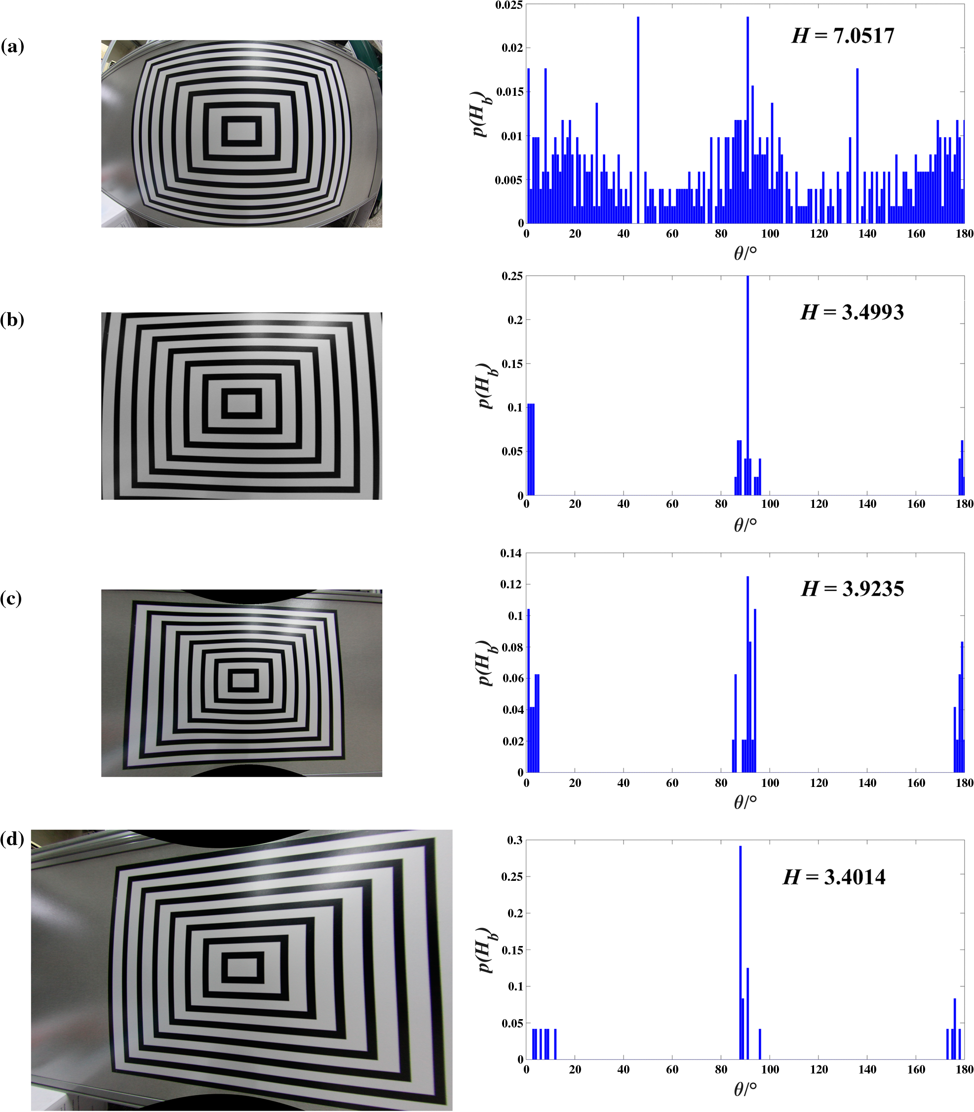

4. Conclusions

In this paper, we proposed an approach for correcting image radial distortion caused by lens. This method works on a single image and does not require a special calibration pattern. Experimental results have shown a significant achievement in correcting image radial distortion in both synthetic and real images. The key contributions of the study can be summarized in three aspects. (1) The proposed method is accurate and robust in estimating radial distortion. It is extremely useful in many applications, particularly for those where human-made environments contain abundant lines. Although the proposed method requires at least three distorted lines residing in an image, it can cope with a situation in which fewer lines are found by adding more images taken by a same camera with different capturing angles. As long as there is a line involved in the scene, the proposed method is applicable. (2) The quantitative evaluation of the estimated radial distortion parameters has been achieved by the defined measure of Hough entropy based on the probability distribution in 1-D $θ$ Hough space. (3) The “Taubin fit” technique has shown its positive effect in the initial guess of an arc’s parameters. It has significantly improved the convergence rate in the process of the LM iterative nonlinear least squares method to calculate an arc’s parameters.

Acknowledgments

This work was supported by the National Natural Science Foundation of China (Grant No. 51575388).

References

1.

J. H. Brito et al., “Radial distortion self-calibration,” in Proc. of the IEEE Conf. on Computer Vision and Pattern Recognition (CVPR ‘13), 1368 –1375 (2013). http://dx.doi.org/10.1109/CVPR.2013.180 Google Scholar

2.

M. R. Bax and R. Shahidi, “Real-time lens distortion correction: speed, accuracy and efficiency,” Opt. Eng., 53 (11), 113103 (2014). http://dx.doi.org/10.1117/1.OE.53.11.113103 Google Scholar

3.

J. Wang et al., “A new calibration model of camera lens distortion,” Pattern Recognit., 41 (2), 607 –615 (2008). http://dx.doi.org/10.1016/j.patcog.2007.06.012 PTNRA8 0031-3203 Google Scholar

4.

F. Wu et al., “Deep space exploration panoramic camera calibration technique based on circular markers,” Acta Opt. Sin., 33 (11), 1115002 (2013). http://dx.doi.org/10.3788/AOS GUXUDC 0253-2239 Google Scholar

5.

Z. Zhang, “A flexible new technique for camera calibration,” IEEE Trans. Pattern Anal. Mach. Intell., 22 (11), 1330 –1334 (2000). http://dx.doi.org/10.1109/34.888718 ITPIDJ 0162-8828 Google Scholar

6.

A. Wang, T. Qiu and L. Shao, “A simple method of radial distortion correction with centre of distortion estimation,” J. Math. Imaging Vision, 35 (3), 165 –172 (2009). http://dx.doi.org/10.1007/s10851-009-0162-1 Google Scholar

7.

F. Devernay and O. Faugeras, “Straight lines have to be straight,” Mach. Vision Appl., 13 (1), 14 –24 (2001). http://dx.doi.org/10.1007/PL00013269 Google Scholar

8.

Z. Kukelova and T. Pajdla, “A minimal solution to radial distortion autocalibration,” IEEE Trans. Pattern Anal. Mach. Intell., 33 (12), 2410 –2422 (2011). http://dx.doi.org/10.1109/TPAMI.2011.86 ITPIDJ 0162-8828 Google Scholar

9.

A. W. Fitzgibbon, “Simultaneous linear estimation of multiple view geometry and lens distortion,” in Proc. of the 2001 IEEE Computer Society Conf. on Computer Vision and Pattern Recognition (CVPR ’01), 125 –132 (2001). http://dx.doi.org/10.1109/CVPR.2001.990465 Google Scholar

10.

D. Claus and A. W. Fitzgibbon, “A rational function lens distortion model for general cameras,” in IEEE Computer Society Conf. on Computer Vision and Pattern Recognition (CVPR ’05), 213 –219 (2005). http://dx.doi.org/10.1109/CVPR.2005.43 Google Scholar

11.

G. P. Stein, “Lens distortion calibration using point correspondences,” in Proc., 1997 IEEE Computer Society Conf. on Computer Vision and Pattern Recognition, 602 –608 (1997). http://dx.doi.org/10.1109/CVPR.1997.609387 Google Scholar

12.

B. Micusik and T. Pajdla, “Structure from motion with wide circular field of view cameras,” IEEE Trans. Pattern Anal. Mach. Intell., 28 (7), 1135 –1149 (2006). http://dx.doi.org/10.1109/TPAMI.2006.151 ITPIDJ 0162-8828 Google Scholar

13.

R. Hartley and S. B. Kang, “Parameter-free radial distortion correction with center of distortion estimation,” IEEE Trans. Pattern Anal. Mach. Intell., 29 (8), 1309 –1321 (2007). http://dx.doi.org/10.1109/TPAMI.2007.1147 ITPIDJ 0162-8828 Google Scholar

14.

S. Ramalingam, P. Sturm and S. K. Lodha, “Generic self-calibration of central cameras,” Comput. Vision Image Understanding, 114 (2), 210 –219 (2010). http://dx.doi.org/10.1016/j.cviu.2009.07.007 CVIUF4 1077-3142 Google Scholar

15.

B. Precott and G. F. McLean, “Line-based correction of radial lens distortion,” Graphical Models Image Process., 59 (1), 39 –47 (1997). http://dx.doi.org/10.1006/gmip.1996.0407 Google Scholar

16.

M. Ahmed and A. Farag, “Nonmetric calibration of camera lens distortion: differential methods and robust estimation,” IEEE Trans. Image Process., 14 (8), 1215 –1230 (2005). http://dx.doi.org/10.1109/TIP.2005.846025 IIPRE4 1057-7149 Google Scholar

17.

Jean-Yves Bouguet, “Camera calibration toolbox for MATLAB,” (2015) http://www.vision.caltech.edu/bouguetj/calib_doc/ October 2016). Google Scholar

18.

D. Li, G. Wen and S. Qiu, “Cross-ratio-based line scan camera calibration using a planar pattern,” Opt. Eng., 55 (1), 014104 (2016). http://dx.doi.org/10.1117/1.OE.55.1.014104 Google Scholar

19.

F. C. M. Alanis and J. A. M. Rodriguez, “Self-calibration of vision parameters via genetic algorithms with simulated binary crossover and laser line projection,” Opt. Eng., 54 (5), 053115 (2015). http://dx.doi.org/10.1117/1.OE.54.5.053115 Google Scholar

20.

J. P. Barreto, “A unifying geometric representation for central projection systems,” Comput. Vision Image Understanding, 103 (3), 208 –217 (2006). http://dx.doi.org/10.1016/j.cviu.2006.06.003 CVIUF4 1077-3142 Google Scholar

21.

F. Bukhari and M. N. Dailey, “Automatic radial distortion estimation from a single image,” J. Math. Imaging Vision, 45 (1), 31 –45 (2013). http://dx.doi.org/10.1007/s10851-012-0342-2 Google Scholar

22.

L. Alvarez et al., “An algebraic approach to lens distortion by line rectification,” J. Math. Imaging Vision, 35 (1), 36 –50 (2009). http://dx.doi.org/10.1007/s10851-009-0153-2 Google Scholar

23.

L. Alvarez, L. Gomez and J. R. Sendra, “Algebraic lens distortion model estimation,” Image Process. On Line, 1 1 –10 (2010). http://dx.doi.org/10.5201/ipol.2010.ags-alde Google Scholar

24.

M. Aleman-Flores et al., “Automatic lens distortion correction using one-parameter division models,” Image Process. On Line, 4 327 –343 (2014). http://dx.doi.org/10.5201/ipol.2014.106 Google Scholar

25.

M. Aleman-Flores et al., “Line detection in images showing significant lens distortion and application to distortion correction,” Pattern Recognit. Lett., 36 261 –271 (2014). http://dx.doi.org/10.1016/j.patrec.2013.06.020 PRLEDG 0167-8655 Google Scholar

26.

D. Santana-Cedres et al., “Invertibility and estimation of two-parameter polynomial and division lens distortion models,” SIAM J. Imaging Sci., 8 (3), 1574 –1606 (2015). http://dx.doi.org/10.1137/151006044 Google Scholar

27.

C. Herrera, J. Kannala and J. Heikkila, “Joint depth and color camera calibration with distortion correction,” IEEE Trans. Pattern Anal. Mach. Intell., 34 (10), 2058 –2064 (2012). http://dx.doi.org/10.1109/TPAMI.2012.125 ITPIDJ 0162-8828 Google Scholar

28.

J. Smisek, M. Jancosek and T. Pajdla, “3D with Kinect,” in IEEE Int. Conf. on Computer Vision Workshops (ICCV Workshops ‘11), 1154 –1160 (2011). http://dx.doi.org/10.1109/ICCVW.2011.6130380 Google Scholar

29.

D. C. Brown, “Decentering distortion of lenses,” Photometric Eng., 32 (3), 444 –462 (1966). Google Scholar

30.

D. C. Brown, “Close-range camera calibration,” Photogramm. Eng., 37 (8), 855 –866 (1971). Google Scholar

31.

J. G. Fryer and D. C. Brown, “Lens distortion for close-range photogrammetry,” Photogramm. Eng. Remote Sens., 52 (1), 51 –58 (1986). Google Scholar

32.

R. Y. Tsai, “A versatile camera calibration technique for high-accuracy 3D machine vision metrology using off-the-shelf TV cameras and lenses,” IEEE J. Rob. Autom., 3 (4), 323 –344 (1987). http://dx.doi.org/10.1109/JRA.1987.1087109 IJRAE4 0882-4967 Google Scholar

33.

T. A. Clarke and J. G. Fryer, “The development of camera calibration methods and models,” Photogrammetric Rec., 16 (91), 51 –66 (1998). http://dx.doi.org/10.1111/phor.1998.16.issue-91 Google Scholar

34.

G. Taubin, “Estimation of planar curves, surfaces and nonplanar space curves defined by implicit equations with applications to edge and range image segmentation,” IEEE Trans. Pattern Anal. Mach. Intell., 13 (11), 1115 –1138 (1991). http://dx.doi.org/10.1109/34.103273 ITPIDJ 0162-8828 Google Scholar

35.

N. Chernov, Circular and Linear Regression: Fitting Circles and Lines by Least Squares, Chapman & Hall/CRC, Boca Raton, Florida (2010). Google Scholar

36.

R. O. Duda and P. E. Hart, “Use of the Hough transformation to detect lines and curves in pictures,” Commun. ACM, 15 (1), 11 –15 (1972). http://dx.doi.org/10.1145/361237.361242 CACMA2 0001-0782 Google Scholar

37.

L. Alvarez, L. Gómez and J. R. Sendra, “Algebraic lens distortion model estimation,” (2015) http://demo.ipol.im/demo/ags_algebraic_lens_distortion_estimation/ September 2016). Google Scholar

38.

Image Processing On Line, (2016) http://www.ipol.im/pub/art/ April ). 2016). Google Scholar

Biography

Fanlu Wu received his BS degree from the School of Opto-Electronic Engineering, Changchun University of Science and Technology, China, in 2011 and his MS degree from the University of the Chinese Academy of Sciences, China, in 2014. He is currently pursuing his PhD in the School of Precision Instrument and Opto-Electronics Engineering, Tianjin University, China. His research interests include camera calibration, image mosaics, and image super-resolution reconstruction.

Hong Wei received her PhD from Birmingham University in 1996. She worked as a postdoctoral research assistant on a Hewlett Packard sponsored project, high-resolution CMOS camera systems. She also worked as a research fellow on an EPSRC-funded Faraday project, model from movies. She joined the University of Reading in 2000. Her current research interest includes intelligent computer vision and its applications in remotely sensed images and face recognition (biometric).

Xiangjun Wang received his BS, MS, and PhD degrees in precision measurement technology and instruments from Tianjin University, China, in 1980, 1985, and 1990, respectively. Currently, he is a professor and director of the precision measurement system research group at Tianjin University. His research interests include photoelectric sensors and testing, computer vision, image analysis, MOEMS, and MEMS.

CC BY: © The Authors. Published by SPIE under a Creative Commons Attribution 4.0 Unported License. Distribution or reproduction of this work in whole or in part requires full attribution of the original publication, including its DOI.

Citation Download Citation

Fanlu Wu, Hong Wei, and Xiangjun Wang "Correction of image radial distortion based on division model," Optical Engineering 56(1), 013108 (24 January 2017). https://doi.org/10.1117/1.OE.56.1.013108

Received: 14 October 2016; Accepted: 5 January 2017; Published: 24 January 2017

Access the abstract

JOURNAL ARTICLE
10 PAGES

DOWNLOAD PAPER SAVE TO MY LIBRARY

GET CITATION

CITATIONS

Cited by 23 scholarly publications.

Explore citations on Lens.org

KEYWORDS

Distortion

Hough transforms

Distributed interactive simulations

Calibration

Image processing

Cameras

Optical engineering

1.

Introduction

2.

Methodology