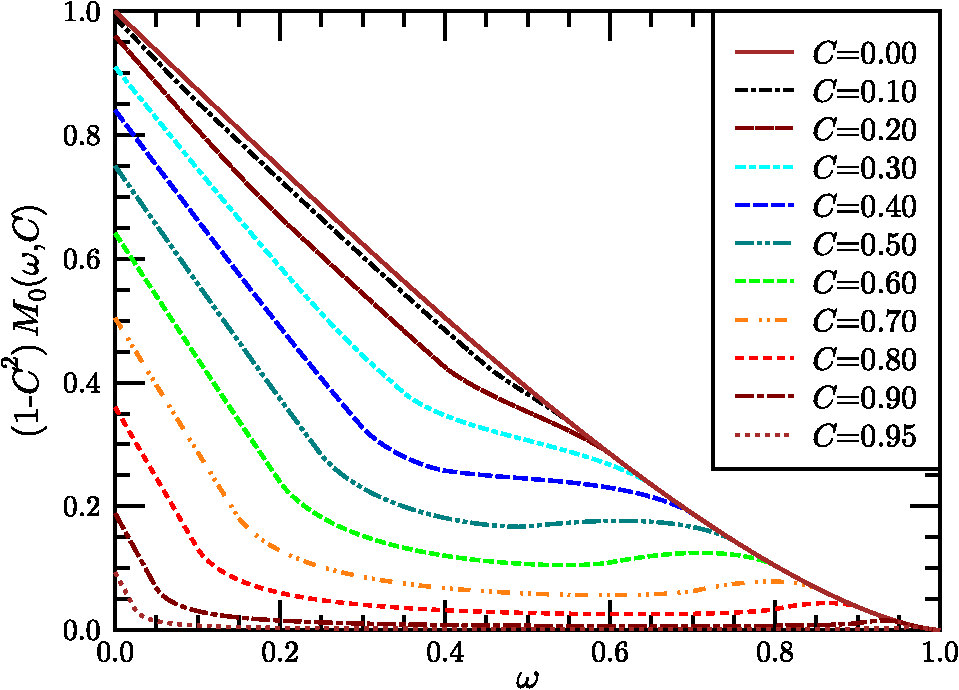
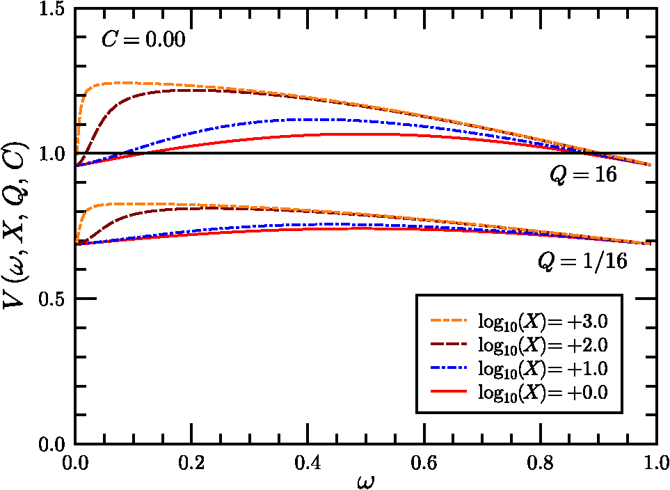
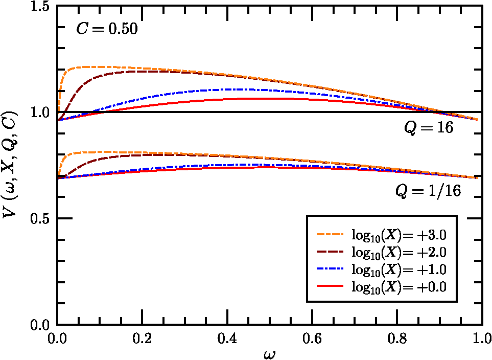
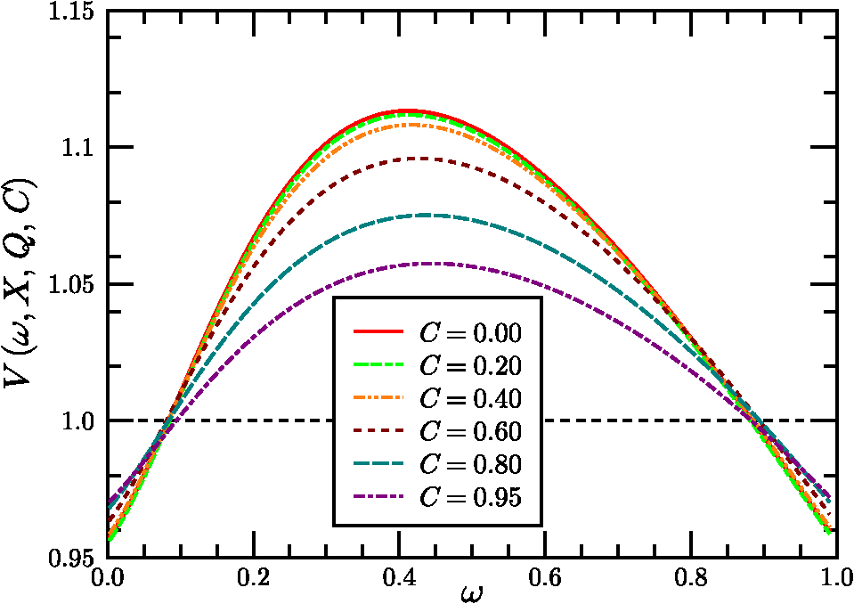
1.

Introduction

The standard theory for modeling atmospheric turbulence impacts in systems performance models^1–3 has been Fried’s⁴ short-exposure atmospheric modulation transfer function (MTF). Reanalysis of Fried’s approach has shown that when diffraction influences on the phase structure function are included,⁵ the tilt-phase (TP) correlation term is numerically evaluated,⁶ and path-dependent turbulence strength variations are considered.⁷ However, like the original Fried work, only circular aperture geometries have been considered. This omits a significant class of telescope optics involving a central obscuration produced by reflector optics’ circularly symmetric secondary mirror. The current paper summarizes efforts to close that gap.

The closest parallel works in the area of optical turbulence effects on annular aperture systems appear to be limited.^8,9 However, these primarily considered the modeling of phase perturbation terms and not the full short-exposure MTF.

The extension of the theory to incorporate this additional effect involves the introduction of a free parameter, here designated as $C$, the ratio of the inner obscuration diameter, $D_1$, to the outer system aperture diameter, $D_2$, such that $0\le C<1$. The limit $C=0$ corresponds to the circular solution.

The revised theory is addressed in general in Sec. 2. Thereafter, individual components of the calculation are considered separately, including the revised system MTF, the tilt-variance calculation, and the TP correlation calculation technique.

2.

Short-Exposure Turbulence Modulation Transfer Function

The short-exposure turbulence MTF (SEMTF), based on Fried’s approach, evaluates the impact of statistically averaged phase and amplitude fluctuations on image quality produced by an optical system. The statistics of the turbulence field is characterized by the wave and phase structure functions, denoted by $\mathcal{D}(r)$ and ${\mathcal{D}}_{\phi }(r)$, respectively. To generate averaged tilt-removed effects, the angle-of-arrival linear phase is mathematically removed. The linear tilt effects are deemed to shift the position of the centroid of the arriving pattern of photons but to not affect image quality. Only the remaining higher order phase and amplitude perturbations produce blur, resulting in MTF degradation.

The engine for the calculations performed involves the Rytov approximation’s (RA) single-scattering model. This method was compared to the reportedly more robust method of Charnotskii¹⁰ in Ref. 6. That paper also discussed limits of the RA based on Dashen’s criteria.¹¹ However, here, for completeness, this discussion will be continued in Sec. 6.

2.1.

Dimensionless Variables Used

The general optical problem encountered is illustrated in Fig. 1. An extended source object plane to be imaged is positioned at $z=-L$. The signal emitted is an incoherent light source consisting of uncorrelated photons, some of which pass through the receiver aperture entrance pupil at $z=0$. The aperture consists of an annular ring whose maximum diameter is $D_2$ and whose inner obscuration diameter is $D_1$. The light studied is monochromatic with wavelength $\lambda$ and wavenumber $k=2\pi /\lambda$, and it passes through an atmosphere characterized by turbulence strength parameter $C_n^2$ (${\mathrm{m}}^{-2/3}$) that in this paper is independent of path position.

Fig. 1

Imaging geometry of the short-exposure imaging problem where optical turbulence fluctuations exist between the object plane and the system entrance pupil.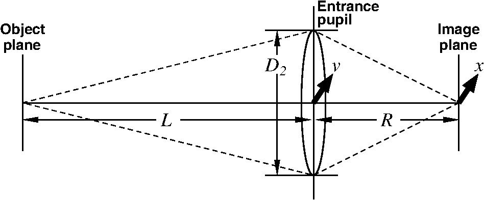

From these variables, we can define a set of dimensionless variables that parameterize the optical problem. First, $C=D_1/D_2$ characterizes the aperture geometry. Second, $Q=D_2/{(\lambda L)}^{1/2}=D_2/F$ parameterizes diffraction influences, where $F$ is the Fresnel zone. Third, $X=D_2/r_o$ characterizes the turbulence strength, where $r_o$ is Fried’s coherence diameter, $r_o=3.018{(k^{2}L{C}_n^2)}^{-3/5}$. To avoid the ubiquitous 2.1 factor, variables ${\rho }_o=r_o/2.1$ (the coherence length) and $S=D_2/{\rho }_o$ will also be used. This model ignores inner- and outer-scale of turbulence effects, whose impacts are minimal for incoherent imaging problems due to the mitigating factors of aperture averaging on the inner scale and aperture size ($D_2<L_o$) on the outer scale. Impacts of path-varying turbulence were considered in Ref. 7.

The final governing variable is the dimensionless angular frequency $\omega$, expressed in radians of frequency per radian of angle: Given a system aperture of outer diameter $D_2$ and wavelength $\lambda$, the maximum angular frequency is denoted ${\mathrm{\Omega }}_o=D_2/\lambda$. This is the upper limit of variable $\mathrm{\Omega }=Rf$ developed by Goodman¹² to aggregate the effects of the system focal length $R$ and spatial frequency $f$ in the system’s image plane. Here, Goodman’s $\mathrm{\Omega }/{\mathrm{\Omega }}_0$ is further reduced to the dimensionless frequency $\omega =\mathrm{\Omega }/{\mathrm{\Omega }}_o$, with limits $0\le \omega \le 1$.

2.3.

Short-Exposure Turbulence Modulation Transfer Function Decomposition

Given these preliminaries, the SEMTF can now be evaluated. In its compact form, the integral expression defining this function is given as^4,5

Eq. (5)

$$\begin{gathered} M_S(\omega )=\frac{1}{A}\int \mathrm{d}\mathbf{v}W(\mathbf{v})W(\mathbf{v}-D_2\mathbf{\omega })\times ⟨\exp \{\ell (\mathbf{v})+\ell (\mathbf{v}-D_2\mathbf{\omega })\}⟩ \\ \times ⟨\exp \{i[\psi (\mathbf{v})-\psi (\mathbf{v}-D_2\mathbf{\omega })]\}⟩, \end{gathered}$$

where $A=\pi D_2^2(1-C^2)/4$ is the area of the system entrance pupil, $W(\mathbf{v})$ are window functions over this pupil, considered as binary functions (0 or 1), $\ell (\mathbf{v})$ is a propagated amplitude perturbation, and $\psi (\mathbf{v})$ is a tilt-corrected phase perturbation. The wavefront tilt over the aperture is characterized by $\mathbf{a}$, such that the tilt-corrected phase function in the system aperture can be expressed as $\psi (\mathbf{v})=\phi (\mathbf{v})-\mathbf{a}·\mathbf{v}$. Fried⁴ showed in detail that $\ell$ and $\psi$ are independent random variables. Angle brackets are used to denote the expectation operator used to create the statistics for the net mean SEMTF.

The factor $A$ imposes a normalization on the SEMTF integral: At zero frequency, $\mathbf{\omega }=0$, we find that

Eq. (6)

$$M_S(0)=\frac{1}{A}\int \mathrm{d}\mathbf{v}{W}^2(\mathbf{v})=1.$$

This result also necessarily assumes $⟨\exp (2\ell )⟩=1$ [see, e.g., Equation (20) of Ref. 5. The principal difference between the short- and long-exposure imaging problems is the presence of $\psi$ that replaces $\phi$ from the long-exposure case. The key element of the analysis of the SEMTF then reduces to the analysis of the expectation functions in Eq. (5). First, note that due to turbulence homogeneity, the relative starting point of these functions is indeterminate. Hence

Eq. (7)

$$⟨\exp \{\ell (\mathbf{v})+\ell (\mathbf{v}-D_2\mathbf{\omega })\}⟩\equiv ⟨\exp \{\ell (0)+\ell (-D_2\mathbf{\omega })\}⟩.$$

Also, because the turbulence is isotropic, the resulting functions will only depend on magnitude $D\omega$. We further define variables $\chi (u)=\ell (0)+\ell (D_{2}u)$ and $\zeta (u)=\psi (0)-\psi (D_{2}u)$. Prior analysis⁴ showed that Eq. (5)’s expectations are expressible in terms of amplitude and tilt-corrected phase structure functions as

Eq. (8)

$$⟨\exp (\chi +i\zeta )⟩=\exp \{-{\mathcal{D}}_{\ell }(v)/2-{\mathcal{D}}_{\psi }(v)/2\}.$$

Variables $\chi$ and $\zeta$ are both Gaussian random variates that are independent of one another. Variable $\zeta$ is also a zero-mean quantity.

The annular aperture window function $W(\mathbf{v})$ can be constructed from a pair of functions $W_o(\mathbf{v}/D)=\mathrm{Cyl}(v/D)$ as

Eq. (9)

$$W(\mathbf{v}/D_2,C)=W_o(\mathbf{v}/D_2)-W_o[(\mathbf{v}/D_2)/C],$$

where $\mathrm{Cyl}(r)=1$, if $r<1/2$ and zero when $r\ge 1/2$. The open portion of the aperture integrates to $A=\pi D_2(1-C^2)/4$. A normalized aperture ($D_2=1$) produces a normalized area $\widehat{A}=\pi (1-C^2)/4$.

Seemingly, the remaining step is to numerically evaluate the integrals with ${\mathcal{D}}_{\ell }(v)$ and ${\mathcal{D}}_{\psi }(v)$. However, upon decomposing ${\mathcal{D}}_{\psi }(D_2\mathbf{\omega })$, we find three terms

Eq. (10)

$$\begin{gathered} {\mathcal{D}}_{\psi }(D_2\mathbf{\omega })=⟨{[\psi (\mathbf{v})-\psi (\mathbf{v}-D_2\mathbf{\omega })]}^2⟩=⟨{\{[\phi (\mathbf{v})-\mathbf{a}·\mathbf{v}]-[\phi (\mathbf{v}-D_2\mathbf{\omega })-\mathbf{a}·(\mathbf{v}-D_2\mathbf{\omega })]\}}^2⟩ \\ =⟨{[\phi (\mathbf{v})-\phi (\mathbf{v}-D_2\mathbf{\omega })]}^2⟩+⟨{[\mathbf{a}·(D_2\mathbf{\omega })]}^2⟩-2⟨[\phi (\mathbf{v})-\phi (\mathbf{v}-D_2\mathbf{\omega })][\mathbf{a}·(D_2\mathbf{\omega })]⟩. \end{gathered}$$

To assess these components, note that the first term on the right is just the phase structure function, ${\mathcal{D}}_{\phi }(D_2\omega )$. Combining this term with the amplitude structure function of Eq. (8) yields a wave structure function. This combined term represents the long-exposure atmospheric turbulence MTF kernel. The remaining terms correspond to the short-exposure corrections. The first of these extra terms (center term on the right) is due to the tilt-variance. However, this term is positive in Eq. (10), which turns negative in Eq. (8), resulting in an overall degradation influence. Therefore, it is the final term on the right in Eq. (10), designated here as the TP correlation, that supplies the counteracting short-exposure correction to long-exposure turbulent blur.

The remaining task involves evaluating these remaining two terms, as well as assessing the net system MTF, defined as $M_0(\omega )$. To facilitate these computations, let us introduce a centered geometry

Eq. (11)

$$M_S(\omega )=\frac{1}{A}\int \mathrm{d}\mathbf{v}W(\mathbf{v}/D_2+\mathbf{\omega }/2,C)W(\mathbf{v}/D_2-\mathbf{\omega }/2,C)\times \exp \{-\mathcal{D}(D_2\omega )/2-\mathrm{TV}+\mathrm{TP}\},$$

where TV is the tilt-variance term and TP is the tilt-phase correlation effect.

In the limit of negligible turbulence, the exponential term in Eq. (11) approaches unity, leaving the system MTF, $M_0(\omega ,C)$, involving the integral of two shifted Eq. (9) window functions. The shifted overlapping windows are illustrated in Fig. 2. The frequency $\omega$ becomes the shift magnitude in the normalized aperture picture ($D_2$ becomes 1/2).

Fig. 2

Intersection of annular apertures displaced center-to-center from one another by amount $\omega$ of unit outer diameter and inner diameter $C=9/14$. Subregions are labeled as $S_1$ through $S_{10}$. Cross marks center of coordinate system (origin of $\mathbf{v}$ vector space).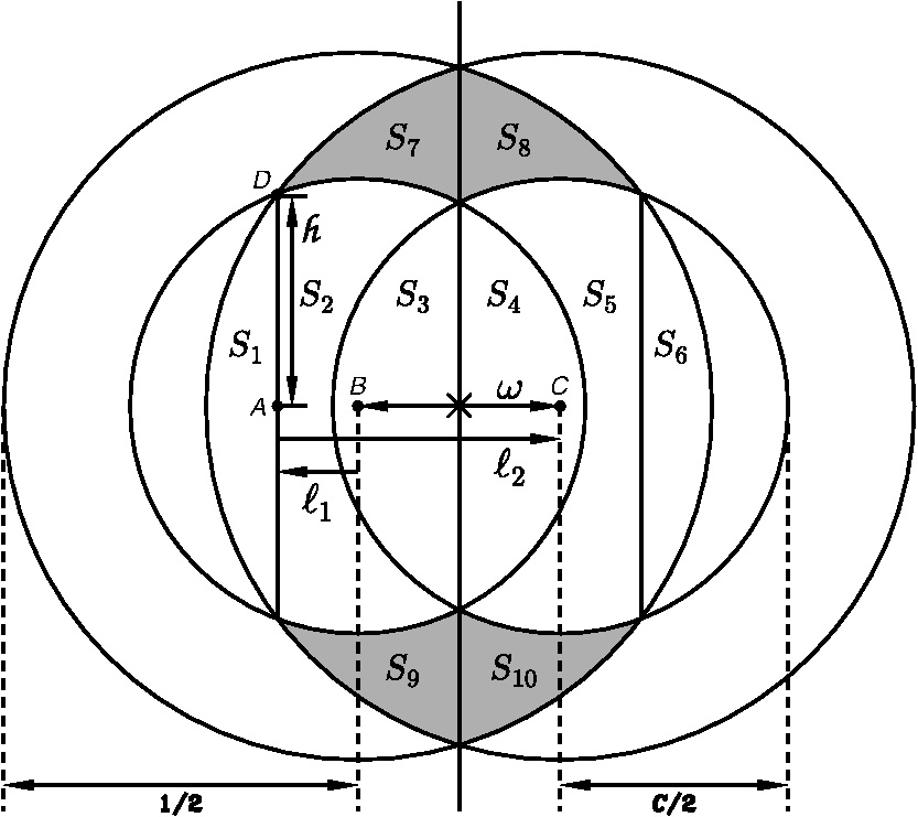

Function $M_0$ appears in integral form as

Eq. (12)

$$M_0(\omega ,C)={\tilde{A}}^{-1}\int \mathrm{d}\mathbf{u}\{W_o[\mathbf{u}+\mathbf{\omega }/2]-W_o[(\mathbf{u}+\mathbf{\omega }/2)/C]\}\{W_o[\mathbf{u}-\mathbf{\omega }/2]-W_o[(\mathbf{u}-\mathbf{\omega }/2)/C]\},$$

where $\mathbf{u}=\mathbf{v}/D_2$. To evaluate this integral, one must simply evaluate the areas of the two outer overlapping circles (the sum of areas $S_1$ through $S_{10}$) plus the overlapping inner circles (areas $S_3$ and $S_4$), then subtract off twice the overlap between an inner and an outer circle (e.g., areas $S_1$ through $S_4$). To evaluate these areas, consider a circle of radius $R$ centered on the origin and integrated from $x=p$ ($-R\le p\le R$) through $x=R$. Let us write this result as

Eq. (13)

$$\tilde{U}(p,R)={\int }_p^{R}2\sqrt{R^2-x^2}\mathrm{d}x=R^2[{\cos }^{-1}(p/R)-(p/R)\sqrt{1-{(p/R)}^2}]=R^{2}U(p/R),$$

where $-R\le p\le +R$. Using this result, for the overlapping outer circles, the net area is

Eq. (14)

$$S_1+\dots +S_{10}=2{(1/2)}^{2}U[(\omega /2)/(1/2)]=U(\omega )/2.$$

The corresponding overlapping inner circle area is

Eq. (15)

$$S_3+S_4=2{(C/2)}^{2}U[(\omega /2)/(C/2)]=C^{2}U(\omega /C)/2,$$

(assuming an overlap exists).

The overlap between inner and outer circles is also evaluated using the $U$ function but requires that arguments ${\ell }_1$ and ${\ell }_2$ be determined. From Fig. 2, if rightward-directed arrows are considered positive valued, leftward arrows as negative valued, and $\omega$ as positive, then

Eq. (16)

$${\ell }_1+{\ell }_2=\omega .$$

To evaluate ${\ell }_1$ and ${\ell }_2$, we also note that right triangles $A\text{-}B\text{-}D$ and $A\text{-}C\text{-}D$ share the common side of length $h$. Side $B\text{-}D$ is $C/2$ long and side $C\text{-}D$ is 1/2 long, leading to the following equations:

Eq. (17)

$${\ell }_1^2+h^2={(C/2)}^2\text{and}{\ell }_2^2+h^2={(1/2)}^2.$$

Subtracting these equations and using symbol $e=e(C)=(1-C^2)/4$

Eq. (18)

$${\ell }_2^2-{\ell }_1^2=e.$$

Equation (16) can be used to eliminate either ${\ell }_1$ or ${\ell }_2$ from Eq. (18), resulting in

Eq. (19)

$${\ell }_1/R_1=K_1(\omega ,C)=({\omega }^2-e)/(C\omega ),{\ell }_2/R_2=K_2(\omega ,C)=({\omega }^2+e)/\omega .$$

These results are directly comparable to the approach of Figs. 9–4 of Ref. 14. These expressions are just the arguments of the related $U$ functions needed to evaluate these areas. Doubling the size of a single inner-outer overlapped area to account for $S_1\text{-}{S}_4$ plus $S_3\text{-}{S}_6$, produces the result

Eq. (20)

$${\mathcal{S}}_{I/O}(\omega ,C)=\left\{\frac{U[K_2(\omega ,C)]+C^{2}U[K_1(\omega ,C)]}{2}\right\}\left[\mathrm{Cyl}\right(\frac{\omega }{1+C})-\mathrm{Cyl}(\frac{\omega }{1-C}\left)\right].$$

Cylinder functions were added to handle the windowing of the function components. For shifts $\omega /2<1-C$, the doubled inner circles lie completely inside the outer circles, whose net contributions are $2\pi C^2/4$. Combining normalized area terms and dividing by $\widehat{A}$ yields the complete system MTF function, written as

Eq. (21)

$$\begin{gathered} M_0(\omega ,C)={\mathcal{G}}_1(\omega ,C)=\frac{2/\pi }{(1-C^2)}[U(\omega )\mathrm{Cyl}(\frac{\omega }{2})+C^{2}U(\omega /C)\mathrm{Cyl}(\frac{\omega }{2C}\left)\right] \\ -\frac{4/\pi }{(1-C^2)}{\mathcal{S}}_{I/O}(\omega ,C)-\frac{2C^2}{(1-C^2)}\mathrm{Cyl}\left(\frac{\omega }{1-C}\right). \end{gathered}$$

Various versions of this function for different choices of parameter $C$ are plotted in Fig. 3. While the basic function is normalized such that $M_0(0,C)=1$, the curves plotted in Fig. 3 have been multiplied by ($1-C^2$) to preserve a sense of the relative entrance pupil in terms of its light-gathering capacity.

Fig. 3

Unnormalized annular aperture system MTF curves for the $C=D_1/D_2$ parameter ranging from 0.0 to 0.95.

The next two sections cover the calculation of the tilt-variance (TV) term in Sec. 3 and the TP correlation term in Sec. 4.

3.

Annular Aperture Tilt-Variance Calculations

In this section, we consider the TV term in Eq. (11). In general, the TV is found to be aperture geometry dependent, but because the turbulence is assumed isotropic and the apertures are circularly symmetric, the tilt statistics is also isotropic ($⟨\mathbf{a}·\mathbf{a}⟩=⟨a_x^2⟩+⟨a_y^2⟩=2⟨a_x^2⟩=2⟨a_y^2⟩$). Components $a_x$ and $a_y$ are also decorrelated ($⟨a_x{a}_y⟩=0$). Therefore, we can write

It remains to evaluate $⟨\mathbf{a}·\mathbf{a}⟩$. To do so, accounting for annular aperture influences, we return to an analysis of Fried’s¹⁵ phase perturbation model. The instantaneous phase perturbation function $\phi (\mathbf{v})$ can be decomposed into an infinite series of weighted orthonormal basis functions

This expression may also be dissected in the form

Fried ordered the $F_{\mu }$ basis functions such that the first few would involve the piston (index 0), tip (1), and tilt (2) terms, such that

Also, ${\mathrm{\Phi }}_0=0$ (no expansion terms), such that ${\mathscr{H}}_0(\mathbf{v})=\phi (\mathbf{v})$. In general, the total unresolved instantaneous phase variance averaged over the system aperture can be evaluated via the integral

In incoherent imaging, once a photon appears on the system image plane, knowledge of the mean phase is lost. Thus, the lowest order measureable phase error is ${\mathrm{\Delta }}_1^2$. Short-exposure imaging further reduces the phase error by eliminating tip and tilt effects since a centroid shift will not reduce point-source image quality. Hence, we focus on ${\mathrm{\Delta }}_3^2$. The difference, ${\mathrm{\Delta }}_1^2-{\mathrm{\Delta }}_3^2=(p_x^2+p_y^2)/A$, is proportional to the TV.

Evaluating this difference involves calculating $p_x$ and $p_y$ coefficients based on integrations using the $F_j$ basis functions. Fried required that these follow the normalization rule

The piston, tip, and tilt terms are given by

The expansion coefficients $p_{\mu }$ are then evaluated using

We then evaluate the two forms from Eq. (32) using the $p_{\mu }$ forms of Eqs. (30) in (26)

The trick involves recognizing that the bracketed region only produces a result for its $F_0(\mathbf{x})$ term in Eq. (34). All other components integrate to zero due to orthogonality. For the zeroth component, the integral evaluates to $A^{1/2}$, which cancels with $F_0=A^{-1/2}$.

Symmetrizing Eq. (34) into the form,

Equations (33) and (35) can be combined to write

Taking the expectation of both sides

At this point, given available space, just the results of further manipulations will be shown. Calculation details were discussed in Ref. 16.

For the circular aperture case, the tilt-variance can be written as

The $G(Q)$ function is parameterized such that it models the main diffraction effects on the tilt-variance while the relative strength of the effect has been aggregated in the leading constant.

The addition of the central obscuration modulates Eq. (41) to the following form:

The third function, $\tilde{G}(Q,C)$, has been similarly formulated as $G(Q)$ so that it approaches a limiting value of unity for large $Q$ but also reflects the influences of $C$. It can be expressed as a modulated version of the original $G(Q)$ function

These functions all have relatively minimal impact [see, e.g., Figs. 6 through 8 of Ref. 16], which is consistent with the concept that tilt effects are dominated by low wavenumber turbulence, with wavelengths wider than the system aperture.

4.

Annular Aperture Tilt-Phase Correlation Calculations

The remaining impact to be quantified from Eq. (11) is the influence of the TP correlation TP. But, in doing so, we recognize, based on Eqs. (24) and (46), that the TV term is independent of the integration variable $\mathbf{v}$ in Eq. (11), as is the wave structure function [first term in the exponential in Eq. (11)]. Therefore, these terms can be factored out of the integral. Conversely, the TP term is dependent on $\mathbf{v}$, and we must write

The full transition to a dimensionless form for TP requires several additional steps. Introducing $\mathbf{a}=W_T\mathbf{p}$ and the Eq. (30) definition of the components into Eq. (10), then using Eq. (10) in the remnants of ${\mathcal{D}}_{\psi }$ in Eq. (8) (gives us a 1/2 factor), and applying isotropic and homogeneous conditions for the structure functions

Introducing dimensionless $\mathbf{u}=\mathbf{v}/D_2$ and rewriting the two phase structure function elements based on Eq. (4)’s decomposition into $J$ and $Y$ functions

To evaluate the integral in Eq. (51), let us divide the window function $\tilde{W}$ into an inner and an outer portion using the form

Finally, to evaluate $M_{\mathrm{TP}}$, we use the following $N$-factor adjustment

5.

Combined Short-Exposure Atmospheric Modulation Transfer Function Model

Sections 3 and 4 developed expressions for the TV and TP components of SEMTF, respectively. Let us summarize these results here. The overall model of the short-exposure expression will be written as

The remaining $M_{\mathrm{TP}}$ effect must be evaluated numerically using Eq. (54). However, rather than leave the results only in this tabulated format, an integrated short-exposure correction term has been developed as a perturbation of the original solution suggested by Fried in treating the circular case

Here, Fried¹⁵ recommended setting the $\tilde{\alpha }$ parameter to either a value of 0.5 or 1.0 (small and large $Q$ cases). Here, the $M_{\mathrm{TV}}$ and $M_{\mathrm{TP}}$ effects are combined to replace Fried’s $\tilde{\alpha }$ by the function $V(\omega ,X,Q,C)$

To tabulate these effects, function $V(\omega ,X,Q,C)$ was evaluated at 103 $\omega$ values, 41 logarithmically increasing $X$ values ranging from 0.1 to ${10}^3$, 9 logarithmically increasing $Q$ values ranging from 1/16 to 16, and 12 $C$ values ranging from 0.00 to 0.95, for a total of 456,084 calculations.

To parameterize the $C$ variability, a parameterized $C$ dependence is constructed for each parameter

The original circular aperture solution was handled as an 80-parameter model. Using the above expression, each of the 80 parameters would need to be characterized by six separate parameters, resulting in a 480-parameter model.

The forms taken by the $V$ at different $C$ values are plotted in a series of graphs below. Figure 4 illustrates samples from the original circular aperture data set. The two groups of lines denote $Q=1/16$ and $Q=16$ behaviors at [essentially] the extents of low $Q$ (high diffraction effects) and high $Q$ (far-field) imaging conditions. (Telescope type systems typically operate in the range of $Q=2\dots 4$.) One finds that the behavior of $V$ does not change significantly above $Q=2$.

Fig. 4

Unnormalized $V(\omega ,X,Q,C)$ for $C=0.00$.

The significant feature of the $V$ curves at high $Q$ values is that they exceed unity over a range of frequencies $\omega$ but fall below unity as $\omega \to 1$. By falling below 1.0 at high frequency, the resulting forms obey diffraction limits, as expected. Conversely, when $V>1$ at intermediate frequencies, one sees a midrange frequency correction of long-exposure turbulence blurring. This recovery is limited to high $Q$ system configurations.

Extending the results illustrated in Fig. 4 to noncircular apertures, Figs. 5 and 6 illustrate behaviors under conditions of moderate ($C=0.50$) and large ($C=0.95$) obstructions. As shown, the main impact of increasing central obscuration is to affect midrange spatial frequencies. $V$ values at these frequencies become increasingly attenuated as $C$ increases. Nonetheless, interestingly, the floor values of the functions (at $\omega =0$ and $\omega =1$ frequencies) remain unaffected.

Fig. 5

Unnormalized $V(\omega ,X,Q,C)$ for $C=0.50$.

Fig. 6

Unnormalized $V(\omega ,X,Q,C)$ for $C=0.95$.

To more directly compare these results, Fig. 7 shows $V$ values from a moderately strong turbulence scenario ($X=10$) for a moderately large aperture ($Q=4$) over a range of $C$ parameter values. Here, $C$ varies from 0.00 to 0.95, but most of the dynamic effects (degradation of the MTF in the high $C$ range) are not significant before $C=0.30$ and are only severe beyond $C=0.50$. Thus, the majority of systems operating at $C\le 0.50$ experience turbulence effects nearly identical to that of circular apertures, differing primarily in terms of the form of the system MTF.

Fig. 7

Plots of $V(\omega ,X,Q,C)$ for varying central obscuration parameter $C$ for $Q=4$ and $X=10$.

To further examine the variability of the $V$ function, let us next note from a comparison of Figs. 5 and 6 how similar the evolution of a given family of $V$ curves is for a given $Q$ and $C$ combination as $X$ ($S$) and $\omega$ are varied. The primary elements that appear to change dramatically are the height of the baseline value of $V$ along with the height of the peak above the baseline. The former is termed $V_0(Q,C)$, and the latter is designated as $V_M(Q,C)$. Figures 8 and 9 illustrate these functional behaviors.

Fig. 8

Plots of minimum $V(\omega ,X,Q,C)$ values ($V_0$) as functions of increasing $Q$ for different aperture central obscuration fractional widths 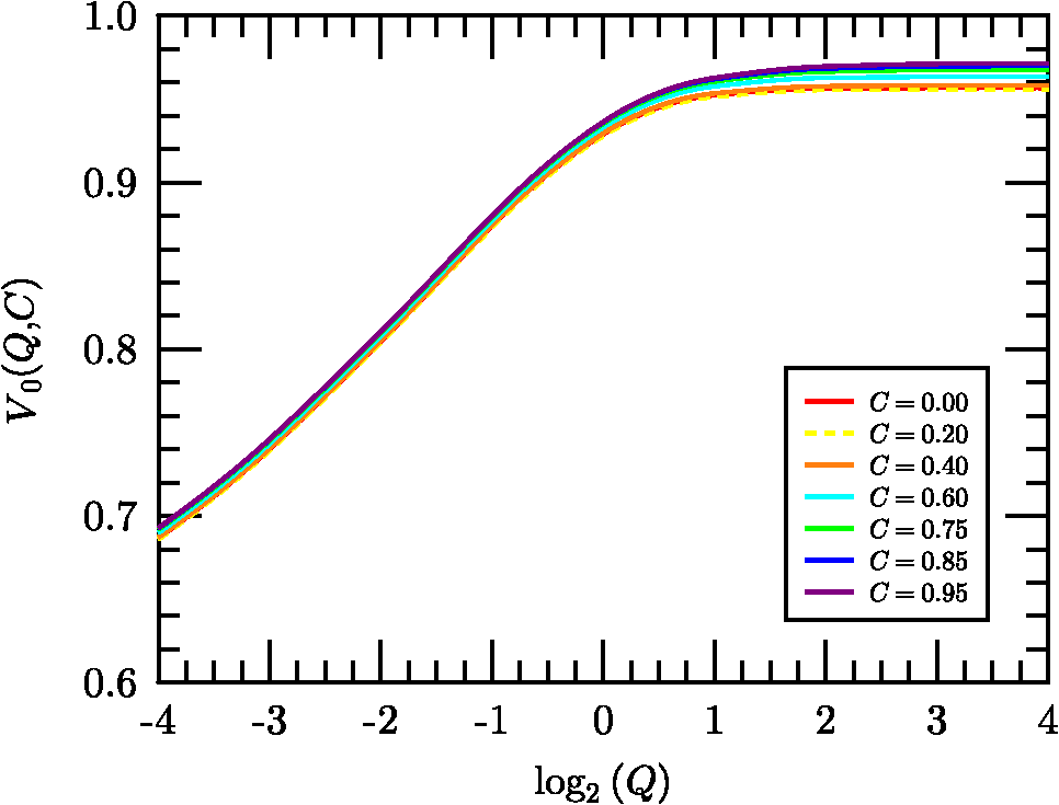$C$.

Fig. 9

Plots of difference between the maximum $V(\omega ,X,Q,C)$ values (captured from the $X=1000$ results) above the minimum $V$ values ($V_0$) for various $Q$ and $C$ combinations.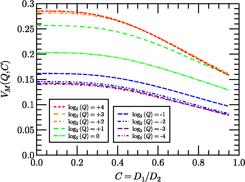

As illustrated in Fig. 8, there are minimal differences in $V_0$ as $C$ varies. The primary driving factor appears to be due to diffraction, as parameterized by its $Q$ variations.

The $V_M$ function appears to exhibit both variations in $C$ and $Q$. As opposed to the $V_0$ function, the influence of the central obscuration can significantly modulate this height. Note, particularly, that increasing $C$ has a degrading effect on the midrange frequency enhancement noted for the circular aperture case. Nonetheless, we find that for relatively large apertures ($Q>2$), there is in fact no value of $C$ that will not produce the needed enhancement to result in $V>1$ at some range of frequencies. On the other hand, if $Q$ is small, e.g., $Q<1/16$, there is no $C$ value that can produce the frequency enhancement region. Also, we see again that for $C<0.3$ and $Q>2$ one finds a plateau region where the behavior of the annular system approximates that of the circular aperture system.

6.

Applicability

Dashen’s¹¹ analysis of the applicability of the RA is now reviewed. Dashen proposed two parameters, $\mathrm{\Phi }$ and $\mathrm{\Theta }$, to describe the influences of diffraction and turbulence on the propagation environment. According to Dashen, if $\mathrm{\Theta }\gg \mathrm{\Phi }$ the RA should apply, where $\mathrm{\Phi }$ represents the rms phase fluctuation using first-order geometric optics to measure turbulence effects and $\mathrm{\Theta }$ represents the diffraction effects due to a characteristic scale size of the turbulence itself. These two parameters were studied in Ref. 6, resulting in the relation

Taking the ratio

Using typical values, this condition is easily achieved (e.g., $L_o\ge 0.5\mathrm{m}$, $C_n^2<{10}^{-12}{\mathrm{m}}^{-2/3}$, $L\le 10\mathrm{km}$). Potvin¹⁷ has further shown recently that RA is consistent with beam steering based on Fermat rays (the Eikonal) affected by large-scale turbulent perturbations.